Non-response and site substitution

A crew draws forty forest plots and reaches thirty-one. Measuring in R what nearest-plot substitution does to survey bias, variance and interval coverage.

A deadwood inventory in a ten kilometre square of state forest. The frame is a grid of forty by forty cells, each a quarter of a kilometre across, and every cell carries a terrain difficulty score worked out before the field season from a digital elevation model and the forest road layer: how steep the ground is and how far it lies from the nearest track. The design is a simple random sample of forty cells, the response is coarse woody debris volume in cubic metres per hectare, and the crew leaves in June with forty grid references.

They come back in September having measured thirty-one of them. One cell was behind a locked gate on private inholding. Two were above a scree slope with no safe line. Three sat across a river that was still in spate in June and never dropped. Three were simply too far from the nearest track to walk in, measure and walk out inside a working day. So the crew did what every field crew does, which is what the protocol told them to do: for each plot they could not reach they went to the nearest plot they could, took the measurements there, and wrote the replacement grid reference on the form.

The sample that comes back therefore has forty rows in it, and forty is the number that goes into the denominator. That is the practice this post is about, and the question is not whether it is untidy but what it costs, measured against a frame whose mean is known.

The nearest thing on this blog is checking a survey design, and it stops just short of this. Its first check compares realised inclusion probabilities with the planned ones, but realised there means realised over repeated draws against the planned frame, which is a property of the draw rather than of the field season. Its third check is about what the frame leaves out before anybody goes anywhere, and in that case there is nothing to substitute, because the units were never candidates. Checking a monitoring design handles a panel that loses sites between years, which is the same idea running along the time axis. What none of them touches is the gap between the sample that was drawn and the sample that came back from a single field season.

One boundary worth drawing before the code starts. Single imputation: bias and variance and the posts around it are about missing values in a table: the unit is present, one of its columns is empty. Here the unit itself is absent, and the thing put in its place is not a guess at a number but a different piece of ground with its own real measurement on it. The vocabulary of missing at random, which Nakagawa and Freckleton (2008) brought across into ecology, carries over; the machinery of imputation does not.

Six treatments of the same forty grid references follow, all against a frame whose true mean is set rather than estimated. Three of them keep the sample at forty by substitution, under three replacement rules that differ only in how the crew chooses where to go instead. Two of them keep the thirty-one and use the frame covariate to repair the loss. One does nothing at all. Then the replacement radius is swept to find where substitution stops paying, the substituted samples are put through the same repair to see whether it still works, and the whole thing is run again under a mechanism that no covariate can reach.

library(ggplot2)

te_pal <- list(forest = "#275139", green = "#2f8f63", sage = "#93a87f",
               clay = "#b5534e", gold = "#cda23f", line = "#dad9ca",
               ink = "#16241d", paper = "#f5f4ee")

theme_te <- function() {
  theme_minimal(base_size = 12) +
    theme(panel.grid.minor = element_blank(),
          panel.grid.major = element_line(colour = "#e7e6dc"),
          plot.background = element_rect(fill = "#f5f4ee", colour = NA),
          panel.background = element_rect(fill = "#f5f4ee", colour = NA),
          plot.title = element_text(face = "bold", colour = te_pal$ink),
          axis.title = element_text(colour = "#2c3a31"),
          axis.text = element_text(colour = "#2c3a31"))
}

A frame, a covariate and a reachable subset

The landscape carries three smooth fields, each built by smoothing white noise on a torus so that neighbouring cells resemble each other over a few hundred metres. The first is terrain difficulty, the covariate the survey has for every cell in the frame. The second stands for everything else that decides whether a crew can get somewhere and that the terrain layer does not know about: ownership, gates, a river crossing. The third is an unrecorded driver of deadwood, standing in for stand history and past management, and it is the field that will matter in the last section. The second and third are orthogonalised against the terrain layer, so any association between them and the covariate in what follows is deliberate rather than accidental.

box_smooth <- function(M, r) {
  nr <- nrow(M); nc <- ncol(M)
  out <- matrix(0, nr, nc)
  for (dr in -r:r) for (dc in -r:r)
    out <- out + M[((seq_len(nr) - 1 - dr) %% nr) + 1,
                   ((seq_len(nc) - 1 - dc) %% nc) + 1]
  out / (2 * r + 1)^2
}
sm_field <- function(sd_side, r1, r2)
  as.vector(scale(as.vector(box_smooth(
    box_smooth(matrix(rnorm(sd_side^2), sd_side, sd_side), r1), r2))))
orth <- function(v, B) as.vector(scale(residuals(lm(v ~ B))))

set.seed(20260731)
side <- 40
n_cell <- side^2
cell_m <- 250
terrain <- sm_field(side, 4, 3)
barrier <- orth(sm_field(side, 4, 3), cbind(terrain))
legacy <- orth(sm_field(side, 4, 3), cbind(terrain, barrier))
cx <- rep(seq_len(side), times = side)
cy <- rep(seq_len(side), each = side)
dmat <- as.matrix(dist(cbind(cx, cy)))

dead <- 20 + 4 * terrain + 3.4 * legacy + rnorm(n_cell, 0, 2)
mu_true <- mean(dead)
print(round(c(cells = n_cell, side_km = side * cell_m / 1000,
              frame_mean = mu_true, frame_sd = sd(dead),
              lowest_cell = min(dead), highest_cell = max(dead),
              cor_terrain = cor(terrain, dead),
              cor_legacy = cor(legacy, dead)), 4))

       cells      side_km   frame_mean     frame_sd  lowest_cell highest_cell 
   1600.0000      10.0000      20.0710       5.5941       5.3828      36.4292 
 cor_terrain   cor_legacy 
      0.7204       0.6003 

Deadwood rises with terrain difficulty because the steep remote compartments are the ones that were never worked, and it rises with the unrecorded legacy field for the same sort of reason. Over the whole frame the mean is 20.071 cubic metres per hectare with a standard deviation of 5.594, the terrain covariate correlates with the response at 0.7204, and that is the number the whole post turns on.

Reachability is a fixed property of a cell rather than a coin tossed on the day: a gate is either locked or it is not. An access score is built as a weighted mix of terrain difficulty and the barrier field, and the easiest part of the frame under that score is declared reachable.

kappa_x <- 0.75
access <- kappa_x * terrain + sqrt(1 - kappa_x^2) * barrier
reach_share <- 0.78
reachable <- access < quantile(access, reach_share)

print(round(c(reachable_share = mean(reachable),
              mean_dead_reachable = mean(dead[reachable]),
              mean_dead_unreachable = mean(dead[!reachable]),
              dead_gap = mean(dead[!reachable]) - mean(dead[reachable]),
              mean_terrain_reachable = mean(terrain[reachable]),
              mean_terrain_unreachable = mean(terrain[!reachable])), 4))

         reachable_share      mean_dead_reachable    mean_dead_unreachable 
                  0.7800                  18.8438                  24.4221 
                dead_gap   mean_terrain_reachable mean_terrain_unreachable 
                  5.5783                  -0.2936                   1.0411 

That leaves 78 per cent of the frame reachable. It holds 18.844 cubic metres per hectare on average and the unreachable remainder 24.422, a gap of 5.578. Any estimator that ends up reporting the reachable mean rather than the frame mean is therefore 1.227 cubic metres per hectare low, and the standard error of a forty-plot mean is a fraction of that, so the error will not be visible in the interval.

One draw, three ways to fill the gap

Draw forty cells at random and see which of them the crew reaches.

n_site <- 40
set.seed(20260801)
drawn <- sample.int(n_cell, n_site)
reached <- drawn[reachable[drawn]]
missed <- drawn[!reachable[drawn]]
print(c(drawn = length(drawn), reached = length(reached), missed = length(missed)))

  drawn reached  missed 
     40      32       8 

print(round(c(mean_terrain_reached = mean(terrain[reached]),
              mean_terrain_missed = mean(terrain[missed]),
              mean_dead_reached = mean(dead[reached]),
              frame_mean = mu_true), 4))

mean_terrain_reached  mean_terrain_missed    mean_dead_reached 
             -0.3086               0.8924              19.2732 
          frame_mean 
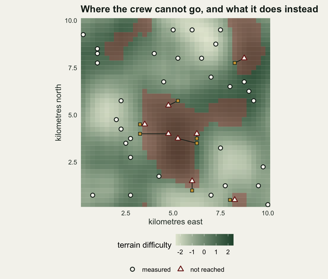
             20.0710 

On this draw 8 of the forty could not be visited, and the crew has to decide where to go instead. Three rules cover most of what happens in practice.

Under the nearest-plot rule the crew walks to the closest cell it can get to that is not already in the sample. This is what a protocol usually says and what a careful crew does. Under the convenience rule it looks around, picks the ground it can actually park next to and work on, and accepts that this might be a kilometre away; that is what happens at four in the afternoon with two plots still on the list. Under the redraw rule nobody walks anywhere: back in the office, fresh cells are drawn from the frame until forty reachable ones are in hand. The redraw is the tidiest of the three on paper and the only one that leaves no trace in the field notebook. Stevens and Olsen (2004) build the same step into the design rather than into the field season, drawing a spatially balanced oversample in advance and working down it in reverse hierarchical order, so that the replacement for a site nobody can reach was chosen before anyone left; the spsurvey package implements both halves of that (Dumelle et al 2023).

sub_lists <- function(reach_flag, ascore, radius, n_cand = 24) {
  ok <- which(reach_flag)
  bad <- which(!reach_flag)
  near <- matrix(0L, length(bad), n_cand)
  easy <- matrix(0L, length(bad), n_cand)
  for (q in seq_along(bad)) {
    dv <- dmat[bad[q], ok]
    ord <- order(dv)
    near[q, ] <- ok[ord[1:n_cand]]
    inr <- which(dv <= radius)
    easy[q, ] <- if (length(inr) >= n_cand)
      ok[inr][order(ascore[ok[inr]])[1:n_cand]]
    else c(ok[inr][order(ascore[ok[inr]])], ok[ord])[1:n_cand]
  }
  row_of <- integer(length(reach_flag))
  row_of[bad] <- seq_along(bad)
  list(near = near, easy = easy, row = row_of)
}

pick_free <- function(cands, taken) {
  for (k in seq_along(cands)) if (!(cands[k] %in% taken)) return(cands[k])
  cands[1]
}

radius_std <- 5
slist <- sub_lists(reachable, access, radius_std)
rows_missed <- slist$row[missed]
near_pick <- integer(0)
for (j in rows_missed) near_pick <- c(near_pick, pick_free(slist$near[j, ], c(reached, near_pick)))
easy_pick <- integer(0)
for (j in rows_missed) easy_pick <- c(easy_pick, pick_free(slist$easy[j, ], c(reached, easy_pick)))

walk_m <- sqrt((cx[near_pick] - cx[missed])^2 + (cy[near_pick] - cy[missed])^2) * cell_m
drive_m <- sqrt((cx[easy_pick] - cx[missed])^2 + (cy[easy_pick] - cy[missed])^2) * cell_m
print(round(c(radius_m = radius_std * cell_m,
              mean_walk_m = mean(walk_m), max_walk_m = max(walk_m),
              mean_drive_m = mean(drive_m)), 1))

    radius_m  mean_walk_m   max_walk_m mean_drive_m 
      1250.0        612.4       1500.0       1281.2 

print(round(c(terrain_missed = mean(terrain[missed]),
              terrain_nearest = mean(terrain[near_pick]),
              terrain_easiest = mean(terrain[easy_pick]),
              terrain_reachable_frame = mean(terrain[reachable])), 4))

         terrain_missed         terrain_nearest         terrain_easiest 
                 0.8924                  0.1069                 -0.8211 
terrain_reachable_frame 
                -0.2936 

The two rules go in opposite directions. On this draw the nearest reachable plots sit at a mean terrain difficulty of 0.1069 against 0.8924 for the plots they replace, so roughly half of what made those plots interesting survives the move. The easiest reachable plots within 1250 metres sit at -0.8211, which is below the average reachable cell in the frame, -0.2936: the crew has not just failed to recover the steep ground, it has gone looking for the flat.

Figure 1: The frame, the reachable subset and one draw of forty plots. Terrain difficulty is shaded from pale where the ground is easy to dark where it is steep and far from a track. The red wash marks the twenty-two per cent of cells the crew cannot reach, which lie mostly over the darker ground. Circles are the plots that were measured, triangles the ones that were not, and each line runs from an unreachable plot to the gold square marking the nearest reachable cell that would replace it.

Six estimates from the same forty grid references

Now the estimators. Three of them analyse the thirty-one reached plots and three of them analyse forty.

Complete case takes the plain mean of the plots that were measured and its usual standard error. Propensity reweighting fits a logistic regression of reached against terrain difficulty over all forty drawn plots, which is possible because the covariate came from the frame and is therefore known for the plots nobody visited, and then weights each measured plot by the reciprocal of its fitted response probability. Post-stratification cuts the frame into four equal terrain quartiles, takes the mean of the measured plots inside each, and combines them with weights that are counts of frame cells rather than counts of plots; strata holding fewer than two measured plots are collapsed into their neighbour, which happens often enough to be worth counting. Haziza and Lesage (2016) set those two weighting procedures side by side and describe the conditions under which each of them repairs a unit non-response. The three substitution estimators take the plain mean of forty and its usual standard error, and differ only in the replacement rule.

n_str <- 4
str_id <- as.integer(cut(terrain, quantile(terrain, seq(0, 1, length.out = n_str + 1)),
                         include.lowest = TRUE))
w_str <- as.vector(table(str_id)) / n_cell

ps_mean <- function(idx) {
  sid <- str_id[idx]
  grp <- seq_len(n_str)
  repeat {
    ug <- unique(grp)
    cnt <- vapply(ug, function(g) sum(grp[sid] == g), 0)
    if (all(cnt >= 2) || length(ug) == 1) break
    b <- ug[which.min(cnt)]
    other <- ug[ug != b]
    grp[grp == b] <- other[which.min(abs(other - b))]
  }
  ug <- unique(grp)
  wg <- vapply(ug, function(g) sum(w_str[grp == g]), 0)
  mg <- vapply(ug, function(g) mean(dead[idx][grp[sid] == g]), 0)
  vg <- vapply(ug, function(g) {
    z <- dead[idx][grp[sid] == g]
    var(z) / length(z)
  }, 0)
  c(sum(wg * mg), sqrt(sum(wg^2 * vg)), max(length(idx) - length(ug), 1),
    n_str - length(ug))
}

one_replicate <- function(reach_flag, sl, seed) {
  set.seed(seed)
  s_draw <- sample.int(n_cell, n_site)
  rch <- s_draw[reach_flag[s_draw]]
  mis <- s_draw[!reach_flag[s_draw]]
  if (length(rch) < 10 || length(mis) < 2) return(NULL)
  plain <- function(ix) c(mean(dead[ix]), sd(dead[ix]) / sqrt(length(ix)))
  cc <- plain(rch)
  fit <- suppressWarnings(glm(reach_flag[s_draw] ~ terrain[s_draw], family = binomial))
  ph <- pmax(as.vector(fitted(fit))[reach_flag[s_draw]], 0.05)
  wg <- 1 / ph
  ipw_m <- sum(wg * dead[rch]) / sum(wg)
  ipw_s <- sqrt(sum(wg^2 * (dead[rch] - ipw_m)^2)) / sum(wg)
  psr <- ps_mean(rch)
  rw <- sl$row[mis]
  a_near <- integer(0)
  for (j in rw) a_near <- c(a_near, pick_free(sl$near[j, ], c(rch, a_near)))
  a_easy <- integer(0)
  for (j in rw) a_easy <- c(a_easy, pick_free(sl$easy[j, ], c(rch, a_easy)))
  a_redr <- sample(setdiff(which(reach_flag), rch), length(mis))
  v_near <- plain(c(rch, a_near))
  v_easy <- plain(c(rch, a_easy))
  v_redr <- plain(c(rch, a_redr))
  q_near <- ps_mean(c(rch, a_near))
  q_easy <- ps_mean(c(rch, a_easy))
  q_redr <- ps_mean(c(rch, a_redr))
  hit <- function(e, se, dfr) abs(e - mu_true) < qt(0.975, dfr) * se
  c(n_reached = length(rch), collapsed = psr[4],
    e_cc = cc[1], s_cc = cc[2], k_cc = hit(cc[1], cc[2], length(rch) - 1),
    e_ipw = ipw_m, s_ipw = ipw_s, k_ipw = hit(ipw_m, ipw_s, length(rch) - 1),
    e_ps = psr[1], s_ps = psr[2], k_ps = hit(psr[1], psr[2], psr[3]),
    e_near = v_near[1], s_near = v_near[2], k_near = hit(v_near[1], v_near[2], n_site - 1),
    e_easy = v_easy[1], s_easy = v_easy[2], k_easy = hit(v_easy[1], v_easy[2], n_site - 1),
    e_redr = v_redr[1], s_redr = v_redr[2], k_redr = hit(v_redr[1], v_redr[2], n_site - 1),
    e_nearps = q_near[1], s_nearps = q_near[2], k_nearps = hit(q_near[1], q_near[2], q_near[3]),
    e_easyps = q_easy[1], s_easyps = q_easy[2], k_easyps = hit(q_easy[1], q_easy[2], q_easy[3]),
    e_redrps = q_redr[1], s_redrps = q_redr[2], k_redrps = hit(q_redr[1], q_redr[2], q_redr[3]),
    terr_gap = mean(terrain[mis]) - mean(terrain[rch]),
    terr_p = t.test(terrain[rch], terrain[mis])$p.value)
}

Two thousand replicates. Each one redraws the forty cells, works out which of them the fixed reachability map allows, and applies all nine analyses to the same field season.

n_rep <- 2000
rep_mat <- do.call(rbind, lapply(seq_len(n_rep),
                                 function(i) one_replicate(reachable, slist, 70000 + i)))
keys <- c("cc", "ipw", "ps", "near", "easy", "redr")
summarise_est <- function(k) {
  e <- rep_mat[, paste0("e_", k)]
  c(bias = mean(e) - mu_true, sd = sd(e), rmse = sqrt(mean((e - mu_true)^2)),
    mean_se = mean(rep_mat[, paste0("s_", k)]),
    coverage = mean(rep_mat[, paste0("k_", k)]))
}
res_tab <- t(sapply(keys, summarise_est))
print(round(res_tab, 4))

        bias     sd   rmse mean_se coverage
cc   -1.2271 0.9587 1.5570  0.9326   0.7425
ipw   0.0477 1.2050 1.2056  1.2553   0.9475
ps   -0.1755 0.8557 0.8732  0.7950   0.9125
near -0.4661 0.8392 0.9598  0.8306   0.9085
easy -1.1884 0.8251 1.4467  0.8096   0.6915
redr -1.2232 0.8376 1.4823  0.8235   0.6860

print(round(c(replicates = nrow(rep_mat), mean_reached = mean(rep_mat[, "n_reached"]),
              stratum_collapse_rate = mean(rep_mat[, "collapsed"] > 0),
              frame_mean = mu_true, reachable_frame_mean = mean(dead[reachable])), 4))

           replicates          mean_reached stratum_collapse_rate 
            2000.0000               31.1330                0.0875 
           frame_mean  reachable_frame_mean 
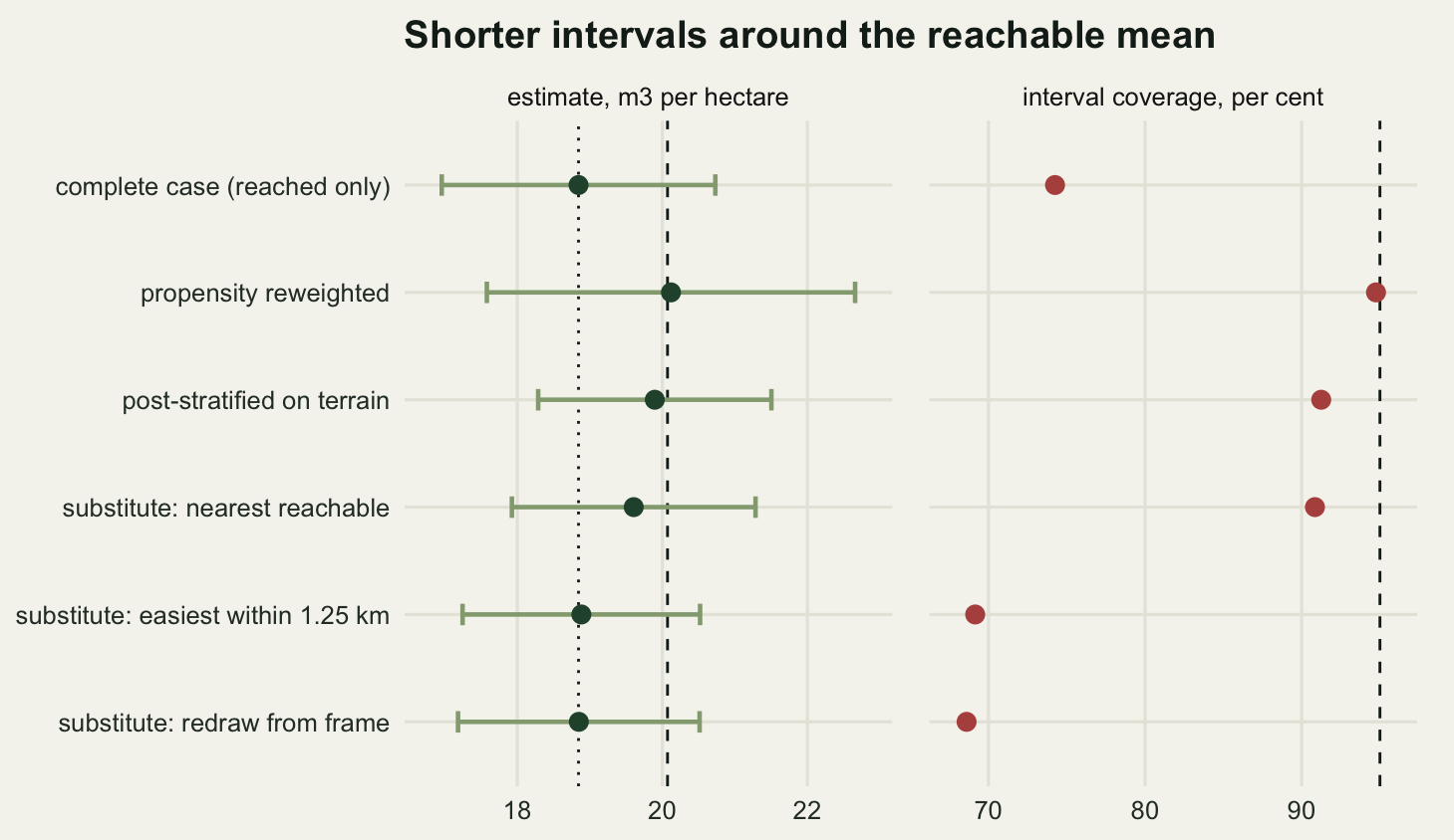
              20.0710               18.8438 

gt <- function(k, col) unname(res_tab[k, col])

Read the table one column at a time. The bias column separates the six into two groups: the two frame-covariate estimators sit at 0.0477 and -0.1755 cubic metres per hectare, nearest-plot substitution at -0.4661, and the other three at -1.2271, -1.1884 and -1.2232. Those last three are all within noise of -1.2272, the exact error of estimating the frame mean by the reachable mean, which is worth holding on to for the next paragraph.

The standard deviation column tells the opposite story. Complete case is the widest at 0.9587 because it is a mean of thirty-one rather than forty; the three substituted estimators are the narrowest of the six, from 0.8251 to 0.8376. Substitution does exactly what it is supposed to do to precision. The mean reported standard error follows the same order, so the interval a reader sees is genuinely shorter: 0.8096 for the convenience rule against 0.9326 for doing nothing.

Put bias and spread together and the coverage column falls out. 94.75 per cent for propensity reweighting and 91.25 per cent for post-stratification, against 74.25 per cent for complete case, 90.85 per cent for the nearest-plot rule, 69.15 per cent for the convenience rule and 68.6 per cent for the redraw. The convenience rule and the redraw carry the same error as doing nothing inside a shorter interval, and shorter intervals around the same wrong number is what a coverage of 68.6 per cent looks like from the inside: the estimator reports more precision because the sample is larger, and the extra precision is aimed at the reachable mean.

same_as_reachable <- c(complete_case = mean(rep_mat[, "e_cc"]),
                       redraw = mean(rep_mat[, "e_redr"]),
                       reachable_frame_mean = mean(dead[reachable]))
mc_se <- sd(rep_mat[, "e_redr"]) / sqrt(nrow(rep_mat))
print(round(same_as_reachable, 4))

       complete_case               redraw reachable_frame_mean 
             18.8439              18.8479              18.8438 

print(round(c(cc_minus_redraw = same_as_reachable[1] - same_as_reachable[2],
              monte_carlo_se = mc_se,
              se_ratio_redraw_over_cc = gt("redr", "mean_se") / gt("cc", "mean_se"),
              rmse_ratio = gt("redr", "rmse") / gt("cc", "rmse")), 5))

cc_minus_redraw.complete_case                monte_carlo_se 
                     -0.00391                       0.01873 
      se_ratio_redraw_over_cc                    rmse_ratio 
                      0.88301                       0.95203 

That agreement is not a coincidence and it does not depend on the numbers. Under a simple random sample the plots that get measured are a simple random sample of the reachable part of the frame, and a fresh draw from the reachable part is the same thing again, so a sample topped up by redrawing is a simple random sample of size forty from the reachable subpopulation. Its expectation is the reachable mean exactly, which is also what complete case estimates. The two averages come out at 18.8439 and 18.8479 against a reachable frame mean of 18.8438, with a Monte Carlo standard error of 0.01873. Redrawing until the sample is full is complete-case deletion with the standard error multiplied by 0.883. It answers the same wrong question with more confidence, and it removes the record that anything went wrong.

The nearest-plot rule is the one result here that goes against the folklore. It cut the bias from -1.2271 to -0.4661, a reduction of 62.01 per cent, and it did that while also being narrower than complete case, so its root mean squared error is 0.9598 against 1.557. I expected substitution to be worse than doing nothing on every measure and it is not, for a reason that is obvious once the map is on the screen: a cell four hundred metres from an unreachable one is still on the flank of the same steep compartment, so the replacement inherits part of the covariate value that made the original plot matter. Proximity is doing statistical work, and whether that work survives depends entirely on how far the crew is allowed to go. Demarest et al (2017) reached a similar verdict from the other end of the discipline, on a national health interview survey in which substituting for the households that would not take part did not move the estimates the way the objection to substitution predicts.

Figure 2: Six analyses of the same forty-plot draw over two thousand simulated field seasons. The left panel shows the mean estimate with the average ninety-five per cent interval; the dashed line is the frame mean and the dotted line the mean of the reachable part of the frame. The right panel shows how often that interval actually contained the frame mean, against the nominal ninety-five per cent. Complete case, the convenience rule and the redraw all estimate the reachable mean; the substituted versions do it inside a shorter interval.

How far the crew may go before substitution stops paying

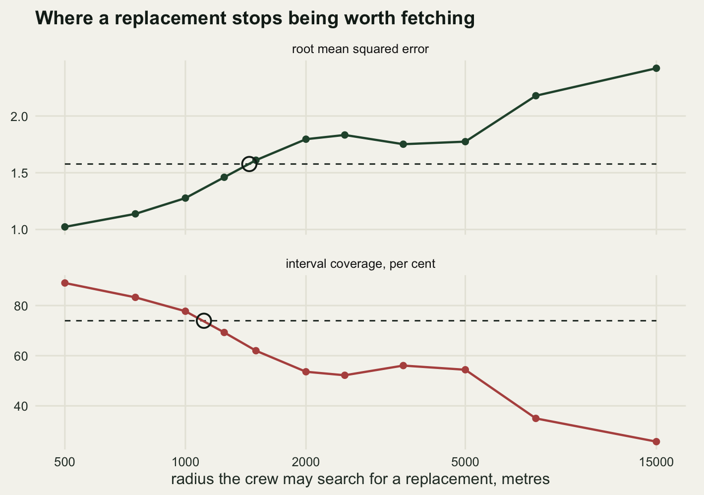
The convenience rule has a dial on it, and the dial is a protocol decision: how far may a crew travel for a replacement. Sweeping it from two cells to the whole frame, with everything else held fixed, gives the exchange rate between convenience and error. At the top of the range the rule degenerates into a roadside survey, because the easiest ground anywhere is where the tracks are.

radius_grid <- c(2, 3, 4, 5, 6, 8, 10, 14, 20, 30, 60)
n_rep_r <- 1500
sweep_r <- do.call(rbind, lapply(radius_grid, function(rr) {
  sl <- sub_lists(reachable, access, rr)
  acc_e <- numeric(n_rep_r)
  acc_k <- numeric(n_rep_r)
  base_e <- numeric(n_rep_r)
  base_k <- numeric(n_rep_r)
  keep <- logical(n_rep_r)
  for (i in seq_len(n_rep_r)) {
    set.seed(310000 + i)
    s_draw <- sample.int(n_cell, n_site)
    rch <- s_draw[reachable[s_draw]]
    mis <- s_draw[!reachable[s_draw]]
    if (length(rch) < 10 || length(mis) < 2) next
    keep[i] <- TRUE
    a_easy <- integer(0)
    for (j in sl$row[mis]) a_easy <- c(a_easy, pick_free(sl$easy[j, ], c(rch, a_easy)))
    ix <- c(rch, a_easy)
    acc_e[i] <- mean(dead[ix])
    acc_k[i] <- abs(acc_e[i] - mu_true) <
      qt(0.975, n_site - 1) * sd(dead[ix]) / sqrt(length(ix))
    base_e[i] <- mean(dead[rch])
    base_k[i] <- abs(base_e[i] - mu_true) <
      qt(0.975, length(rch) - 1) * sd(dead[rch]) / sqrt(length(rch))
  }
  c(radius_m = rr * cell_m,
    terrain_sub = mean(terrain[sl$easy[, 1]]),
    bias = mean(acc_e[keep]) - mu_true,
    rmse = sqrt(mean((acc_e[keep] - mu_true)^2)),
    coverage = mean(acc_k[keep]),
    rmse_cc = sqrt(mean((base_e[keep] - mu_true)^2)),
    coverage_cc = mean(base_k[keep]))
}))
print(round(sweep_r, 4))

      radius_m terrain_sub    bias   rmse coverage rmse_cc coverage_cc
 [1,]      500      0.3712 -0.5589 1.0227   0.8900  1.5768      0.7393
 [2,]      750      0.1565 -0.7434 1.1376   0.8327  1.5768      0.7393
 [3,]     1000     -0.0994 -0.9390 1.2766   0.7773  1.5768      0.7393
 [4,]     1250     -0.3877 -1.1839 1.4600   0.6927  1.5768      0.7393
 [5,]     1500     -0.6443 -1.3650 1.6105   0.6200  1.5768      0.7393
 [6,]     2000     -1.0622 -1.5771 1.7957   0.5360  1.5768      0.7393
 [7,]     2500     -1.2477 -1.6202 1.8328   0.5220  1.5768      0.7393
 [8,]     3500     -1.1492 -1.5411 1.7515   0.5607  1.5768      0.7393
 [9,]     5000     -0.9831 -1.5685 1.7741   0.5440  1.5768      0.7393
[10,]     7500     -1.3500 -2.0060 2.1787   0.3500  1.5768      0.7393
[11,]    15000     -1.5292 -2.2643 2.4210   0.2573  1.5768      0.7393

crossing <- function(d, xax) {
  sg <- sign(d)
  j <- which(sg[-1] != sg[-length(sg)])[1]
  if (is.na(j)) return(NA_real_)
  xax[j] + (xax[j + 1] - xax[j]) * (0 - d[j]) / (d[j + 1] - d[j])
}
cross_rmse <- crossing(sweep_r[, "rmse"] - sweep_r[, "rmse_cc"], sweep_r[, "radius_m"])
cross_cov <- crossing(sweep_r[, "coverage"] - sweep_r[, "coverage_cc"], sweep_r[, "radius_m"])
print(round(c(rmse_crossing_m = cross_rmse, coverage_crossing_m = cross_cov), 1))

    rmse_crossing_m coverage_crossing_m 
             1444.0              1112.2 

At a radius of 500 metres the convenience rule is close to the nearest-plot rule and it helps: root mean squared error 1.0227 against 1.5768 for doing nothing, and coverage 89 per cent against 73.93 per cent. Let the crew go far enough and both advantages reverse. The root mean squared error of the substituted estimate overtakes complete-case deletion at a radius of 1444 metres, and its coverage falls below complete case earlier still, at 1112 metres. Past that point the substituted sample is not a partial repair of the loss; it is a worse answer than the crew would have brought back by going home.

The far end of the sweep is the roadside survey. With no radius limit the replacements are the easiest cells in the frame, at a mean terrain difficulty of -1.5292, and the estimate is 2.2643 cubic metres per hectare low with a coverage of 25.73 per cent. Fewer than a quarter of the plots had to move to do that, which is the same arithmetic Kadmon, Farber and Danin (2004) measured when they compared roadside records with off-road ones against distribution models: the fifth of the sample nobody could reach is not a fifth of the information.

Figure 3: Error and coverage of the convenience substitution rule against the radius the crew is allowed to search, with complete-case deletion as the horizontal reference in each panel. Both curves cross the reference between one and one and a half kilometres. Below that radius substitution repairs part of the loss; above it the substituted sample is further from the truth than the reached plots alone, and its interval is shorter.

The other dial is the one the survey does not control: how strongly reachability is tied to the response. That coupling, rather than the size of the loss, is what decides whether a loss costs anything, which is the point Groves (2006) established for household surveys by assembling the studies that had measured both. Sweeping it here, with the radius held at 1250 metres, produces no crossing at all.

kappa_grid <- c(0, 0.15, 0.3, 0.45, 0.6, 0.75, 0.9)
n_rep_k <- 1000
sweep_k <- do.call(rbind, lapply(seq_along(kappa_grid), function(q) {
  kk <- kappa_grid[q]
  asc <- kk * terrain + sqrt(1 - kk^2) * barrier
  rf <- asc < quantile(asc, reach_share)
  sl <- sub_lists(rf, asc, radius_std)
  ests <- matrix(NA_real_, n_rep_k, 4)
  for (i in seq_len(n_rep_k)) {
    set.seed(400000 + 3000 * q + i)
    s_draw <- sample.int(n_cell, n_site)
    rch <- s_draw[rf[s_draw]]
    mis <- s_draw[!rf[s_draw]]
    if (length(rch) < 10 || length(mis) < 2) next
    a_near <- integer(0)
    for (j in sl$row[mis]) a_near <- c(a_near, pick_free(sl$near[j, ], c(rch, a_near)))
    a_easy <- integer(0)
    for (j in sl$row[mis]) a_easy <- c(a_easy, pick_free(sl$easy[j, ], c(rch, a_easy)))
    a_redr <- sample(setdiff(which(rf), rch), length(mis))
    ests[i, ] <- c(mean(dead[rch]), mean(dead[c(rch, a_near)]),
                   mean(dead[c(rch, a_easy)]), mean(dead[c(rch, a_redr)]))
  }
  ests <- ests[complete.cases(ests), ]
  rmse_of <- function(v) sqrt(mean((v - mu_true)^2))
  c(kappa = kk, dead_gap = mean(dead[!rf]) - mean(dead[rf]),
    rmse_cc = rmse_of(ests[, 1]), rmse_near = rmse_of(ests[, 2]),
    rmse_easy = rmse_of(ests[, 3]), rmse_redr = rmse_of(ests[, 4]))
}))
print(round(sweep_k, 4))

     kappa dead_gap rmse_cc rmse_near rmse_easy rmse_redr
[1,]  0.00   0.6448  1.0242    0.9340    0.9259    0.9115
[2,]  0.15   1.7933  1.0941    0.9502    1.0322    0.9700
[3,]  0.30   2.7219  1.1419    0.9497    1.1048    1.0329
[4,]  0.45   3.5892  1.2892    0.9709    1.2327    1.1962
[5,]  0.60   4.3663  1.3696    0.9358    1.3001    1.2832
[6,]  0.75   5.5783  1.5229    0.9304    1.4113    1.4746
[7,]  0.90   6.6384  1.7385    0.9319    1.4605    1.6658

worst_margin <- max(c(sweep_k[, "rmse_near"], sweep_k[, "rmse_easy"],
                      sweep_k[, "rmse_redr"]) - rep(sweep_k[, "rmse_cc"], 3))
print(round(c(worst_easy_margin = max(sweep_k[, "rmse_easy"] - sweep_k[, "rmse_cc"]),
              worst_redr_margin = max(sweep_k[, "rmse_redr"] - sweep_k[, "rmse_cc"]),
              worst_near_margin = max(sweep_k[, "rmse_near"] - sweep_k[, "rmse_cc"]),
              worst_of_all = worst_margin), 4))

worst_easy_margin worst_redr_margin worst_near_margin      worst_of_all 
          -0.0371           -0.0482           -0.0901           -0.0371 

Across the whole sweep, from a landscape where reachability says nothing about deadwood to one where the unreachable fifth holds 6.638 cubic metres per hectare more than the rest, the closest any substitution rule comes to losing is an excess root mean squared error of -0.0371 over complete-case deletion. That is a negative number: none of the three ever loses. This is the measurement I set out expecting to come out the other way. Substitution does not make the point estimate worse than dropping the unreached plots, because it buys sample size and, in the nearest-plot case, borrows the covariate as well. What it makes worse is the interval, every time, and the interval is what a survey report is for.

A substituted sample can still be repaired

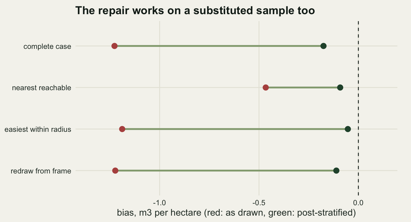
If a crew comes back with forty plots, some of which are substitutes, is the season wasted? The replacement cells have terrain difficulty values of their own, and the frame still knows how many cells sit in each terrain quartile. Post-stratification only needs those two things, so it can be run on a substituted sample exactly as it is run on a reached-only one. The three post-stratified substitution estimators were computed alongside the others in the replicate loop above.

pairs_tab <- rbind(
  "complete case" = c(res_tab["cc", c("bias", "rmse", "coverage")],
                      res_tab["ps", c("bias", "rmse", "coverage")]),
  "nearest reachable" = c(res_tab["near", c("bias", "rmse", "coverage")],
                          summarise_est("nearps")[c("bias", "rmse", "coverage")]),
  "easiest within radius" = c(res_tab["easy", c("bias", "rmse", "coverage")],
                              summarise_est("easyps")[c("bias", "rmse", "coverage")]),
  "redraw from frame" = c(res_tab["redr", c("bias", "rmse", "coverage")],
                          summarise_est("redrps")[c("bias", "rmse", "coverage")]))
colnames(pairs_tab) <- c("bias_raw", "rmse_raw", "cover_raw",
                         "bias_ps", "rmse_ps", "cover_ps")
print(round(pairs_tab, 4))

                      bias_raw rmse_raw cover_raw bias_ps rmse_ps cover_ps
complete case          -1.2271   1.5570    0.7425 -0.1755  0.8732   0.9125
nearest reachable      -0.4661   0.9598    0.9085 -0.0915  0.6732   0.9400
easiest within radius  -1.1884   1.4467    0.6915 -0.0530  0.7506   0.9195
redraw from frame      -1.2232   1.4823    0.6860 -0.1108  0.7320   0.9315

best_raw <- rownames(pairs_tab)[which.min(pairs_tab[, "rmse_raw"])]
best_ps <- rownames(pairs_tab)[which.min(pairs_tab[, "rmse_ps"])]
print(c(best_analysed_as_drawn = best_raw, best_post_stratified = best_ps))

best_analysed_as_drawn   best_post_stratified 
   "nearest reachable"    "nearest reachable" 

print(round(c(gain_over_reached_only =
                pairs_tab["complete case", "rmse_ps"] /
                pairs_tab["nearest reachable", "rmse_ps"]), 4))

gain_over_reached_only 
                1.2971 

Post-stratification pulls every one of the four back towards the truth. The convenience rule goes from a bias of -1.1884 to -0.053 and its coverage from 69.15 to 91.95 per cent; the redraw from -1.2232 to -0.1108. The mechanism is not subtle: a substituted sample is short of plots in the hardest terrain quartile and holds too many in the easiest, and reweighting by frame cell counts is precisely the correction for that.

The best of the eight analyses is nearest-plot substitution post-stratified, at a root mean squared error of 0.6732 against 0.8732 for the same repair applied to the reached plots alone, a factor of 1.2971. Once the covariate is used, the extra plots stop being a disguise and start being data. That is the practical reading of the whole table: substitution is not the mistake. Substitution analysed as though the drawn sample had been measured is the mistake, and the two are separated by writing down which grid references were replaced and what the covariate said about each.

Figure 4: Bias of four field outcomes before and after post-stratification on the terrain covariate, over the same two thousand replicates. Each line runs from the estimate as it would be reported if the sample were analysed as drawn to the estimate after reweighting by frame cell counts. All four move towards zero, and the substituted samples end closer to it than the reached plots alone because they carry more plots.

What none of this can see

Every correction above leans on one assumption: that whatever made a plot unreachable is captured by the terrain covariate the frame carries. Build a landscape where it is not, and nothing changes on the surface. The second mechanism below ties reachability to the legacy field, the unrecorded driver of deadwood, and its strength is tuned so that the gap in deadwood between the reachable and unreachable parts of the frame matches the first mechanism as closely as the grid allows. The damage to the survey is the same. The trace it leaves in the terrain covariate is not.

a_grid <- seq(0.5, 1, by = 0.01)
gap_target <- mean(dead[!reachable]) - mean(dead[reachable])
gap_of <- function(a) {
  sc <- a * legacy + sqrt(1 - a^2) * barrier
  rf <- sc < quantile(sc, reach_share)
  mean(dead[!rf]) - mean(dead[rf])
}
a_star <- a_grid[which.min(abs(vapply(a_grid, gap_of, 0) - gap_target))]
access2 <- a_star * legacy + sqrt(1 - a_star^2) * barrier
reach2 <- access2 < quantile(access2, reach_share)
slist2 <- sub_lists(reach2, access2, radius_std)
print(round(c(a_star = a_star,
              dead_gap_recorded = gap_target,
              dead_gap_unrecorded = mean(dead[!reach2]) - mean(dead[reach2]),
              terrain_gap_recorded = mean(terrain[!reachable]) - mean(terrain[reachable]),
              terrain_gap_unrecorded = mean(terrain[!reach2]) - mean(terrain[reach2])), 4))

                a_star      dead_gap_recorded    dead_gap_unrecorded 
                0.8900                 5.5783                 5.6374 
  terrain_gap_recorded terrain_gap_unrecorded 
                1.3347                 0.0196 

rep_mnar <- do.call(rbind, lapply(seq_len(n_rep),
                                  function(i) one_replicate(reach2, slist2, 80000 + i)))
mnar_tab <- t(sapply(c("cc", "ipw", "ps", "near", "nearps"), function(k) {
  e <- rep_mnar[, paste0("e_", k)]
  c(bias = mean(e) - mu_true, rmse = sqrt(mean((e - mu_true)^2)),
    coverage = mean(rep_mnar[, paste0("k_", k)]))
}))
print(round(mnar_tab, 4))

          bias   rmse coverage
cc     -1.1866 1.4775   0.7508
ipw    -1.1829 1.4404   0.7653
ps     -1.2670 1.4057   0.4695
near   -0.7434 1.1064   0.8589
nearps -0.6384 0.8385   0.7998

The two mechanisms remove almost identical amounts of deadwood from the reachable part of the frame, 5.578 cubic metres per hectare against 5.637. Under the first, propensity reweighting brought the bias to 0.0477. Under the second it brings it to -1.1829, against -1.1866 for doing nothing: the correction removes 0.31 per cent of the problem. Post-stratification does something worse than nothing, holding the bias at -1.267 while tightening the interval, so its coverage falls to 46.95 per cent against 75.08 per cent for the plain mean of the reached plots. A correction that cannot see the mechanism still narrows the interval, and narrowing an interval around a biased estimate is the one operation that makes a survey worse in both directions at once.

One thing does survive. The nearest-plot rule cuts the bias to -0.7434 here as well, and post-stratifying it afterwards reaches -0.6384 with a coverage of 79.98 per cent. It survives because it borrows from geography rather than from a recorded variable, and the unrecorded driver is spatially smooth like everything else in this landscape. That is a real property of a real correction and it is also its limit: it works to the extent that the missing driver varies slowly in space, and nothing in the reached data says whether it does.

So there is no test to run afterwards. What there is, and it is more than most missing-data problems offer, is the frame. The frame holds a covariate for every cell that was drawn, including the nine nobody reached, so the two groups can be compared directly. That comparison is one line, and it is a different line from anything an analyst can do with the measured values.

check_tab <- rbind(
  recorded = c(mean_terrain_gap = mean(rep_mat[, "terr_gap"]),
               detected = mean(rep_mat[, "terr_p"] < 0.05, na.rm = TRUE)),
  unrecorded = c(mean_terrain_gap = mean(rep_mnar[, "terr_gap"]),
                 detected = mean(rep_mnar[, "terr_p"] < 0.05, na.rm = TRUE)))
print(round(check_tab, 4))

           mean_terrain_gap detected
recorded             1.3357   0.9800
unrecorded           0.0096   0.0495

Under the recorded mechanism the nine unreached plots sit 1.3357 terrain standard deviations above the thirty-one that were measured, and a two-sample test on that difference fires in 98 per cent of field seasons, on about nine unreached plots against about thirty-one reached. Under the unrecorded mechanism the same gap is 0.0096 and the test fires at 4.95 per cent, which is the false positive rate and nothing else. The check is worth running because a positive result tells you the weighting has something to work with. A negative result tells you nothing at all, and in particular does not tell you the loss was harmless: the second landscape passes it every time while carrying exactly as much bias as the first.

What to take away

The result that surprised me is that substitution does not make the point estimate worse than dropping the unreached plots. Over the whole coupling sweep no substitution rule ever lost to complete-case deletion on root mean squared error, and the nearest-plot rule cut the bias by 62.01 per cent because a cell a few hundred metres away is still on the same hillside. The folk objection to substitution, that you are inventing data, is aimed at the wrong quantity.

What holds up is the damage to the interval. Substitution restores the denominator, so the reported standard error falls, and if the replacement rule has not also removed the bias then the interval is shorter around the same wrong number. Coverage went from 74.25 per cent for complete case to 68.6 per cent for the redraw and 69.15 per cent for the convenience rule, against a nominal ninety-five. The redraw is the clean case: because a topped-up sample is a simple random sample of the reachable subpopulation, it estimates exactly what complete case estimates, 18.8479 against 18.8439, with the standard error multiplied by 0.883.

Distance is a protocol decision, and it decides which of those two applies. Convenience substitution helps while the crew stays close and hurts once it does not, and on this frame the two lines cross at 1444 metres for error and 1112 metres for coverage. A replacement rule with no distance limit is a roadside survey wearing a probability sample’s clothes: at the far end of the sweep the estimate was 2.2643 cubic metres per hectare low with 25.73 per cent coverage.

The repair is cheap and it works on substituted samples. Post-stratifying on the frame covariate moved all four field outcomes to within 0.1755 cubic metres per hectare of the truth, and the best analysis of the eight was nearest-plot substitution post-stratified, at a root mean squared error 1.2971 times better than the same repair on the reached plots alone. It needs two things that cost nothing in the field: the covariate value for every cell that was drawn, which the frame already has, and a record of which grid references were replaced, which the crew already knows and usually does not write down.

The honest limit is that none of the repairs works when reachability tracks the response through something the frame does not record. Tying reachability to an unrecorded driver instead of to terrain produced the same 5.637 cubic metre per hectare gap and left propensity reweighting at -1.1829 against -1.1866 for doing nothing, while post-stratification tightened the interval around an unmoved bias and dropped coverage to 46.95 per cent. Nothing in the measured plots separates that world from the first one. The frame does part of the job: comparing the covariate of the plots that were measured against the plots that were not took one line and fired in 98 per cent of seasons under the recorded mechanism and 4.95 per cent under the unrecorded one. Run it, report it, and read a null result as silence rather than as clearance.

References

Stevens DL, Olsen AR 2004 Journal of the American Statistical Association 99(465):262-278 (10.1198/016214504000000250)

Groves RM 2006 Public Opinion Quarterly 70(5):646-675 (10.1093/poq/nfl033)

Haziza D, Lesage E 2016 Journal of Official Statistics 32(1):129-145 (10.1515/jos-2016-0006)

Demarest S, Molenberghs G, Van der Heyden J, Gisle L, Van Oyen H, de Waleffe S, Van Hal G 2017 International Journal of Public Health 62(8):949-957 (10.1007/s00038-017-0976-3)

Kadmon R, Farber O, Danin A 2004 Ecological Applications 14(2):401-413 (10.1890/02-5364)

Nakagawa S, Freckleton RP 2008 Trends in Ecology and Evolution 23(11):592-596 (10.1016/j.tree.2008.06.014)

Dumelle M, Kincaid T, Olsen AR, Weber M 2023 Journal of Statistical Software 105(3):1-29 (10.18637/jss.v105.i03)

Related tutorials

• Checking a survey design
• Checking a monitoring design
• Checking a stratified design
• Missing data: MCAR, MAR and MNAR