Single imputation: bias and variance

Why single imputation misleads in R: mean imputation attenuates the slope, regression imputation inflates correlations, and one completed dataset always understates uncertainty.

Filling a gap with a single plausible number and carrying on as if the value were real is the most tempting fix for missing data, and the most quietly damaging. This post works through three single-imputation methods, mean imputation, regression imputation, and its stochastic version, and shows two separate failures: some methods bias the estimate you care about, and all of them understate its uncertainty. The second failure is the harder one to see, and it is the reason the next post moves to multiple imputation.

The setting is a response y that is missing at random given an observed predictor x, with the slope of y on x as the quantity of interest (true value 1.5).

The data and the three fills

set.seed(2947)
n <- 500; c0 <- 1; c1 <- 1.5; sdx <- 1.2; sde <- 1.6
x <- rnorm(n, 0, sdx)
y <- c0 + c1 * x + rnorm(n, 0, sde)
full_slope <- unname(coef(lm(y ~ x))[2]); full_r <- cor(x, y); full_sdY <- sd(y)

## missing at random: higher x makes y more likely to be missing (about 40%)
a1 <- 1.1
a0 <- uniroot(function(a) mean(plogis(a + a1 * x)) - 0.40, c(-5, 5))$root
miss <- runif(n) < plogis(a0 + a1 * x); obs <- !miss

impute <- function(kind) {
  yo <- y; yo[miss] <- NA
  fit <- lm(yo[obs] ~ x[obs]); sig <- summary(fit)$sigma
  yhat <- coef(fit)[1] + coef(fit)[2] * x[miss]
  if (kind == "mean")   yo[miss] <- mean(y[obs])                        # constant fill
  if (kind == "detreg") yo[miss] <- yhat                               # on the fitted line
  if (kind == "stoch")  yo[miss] <- yhat + rnorm(sum(miss), 0, sig)     # line plus residual noise
  yo
}

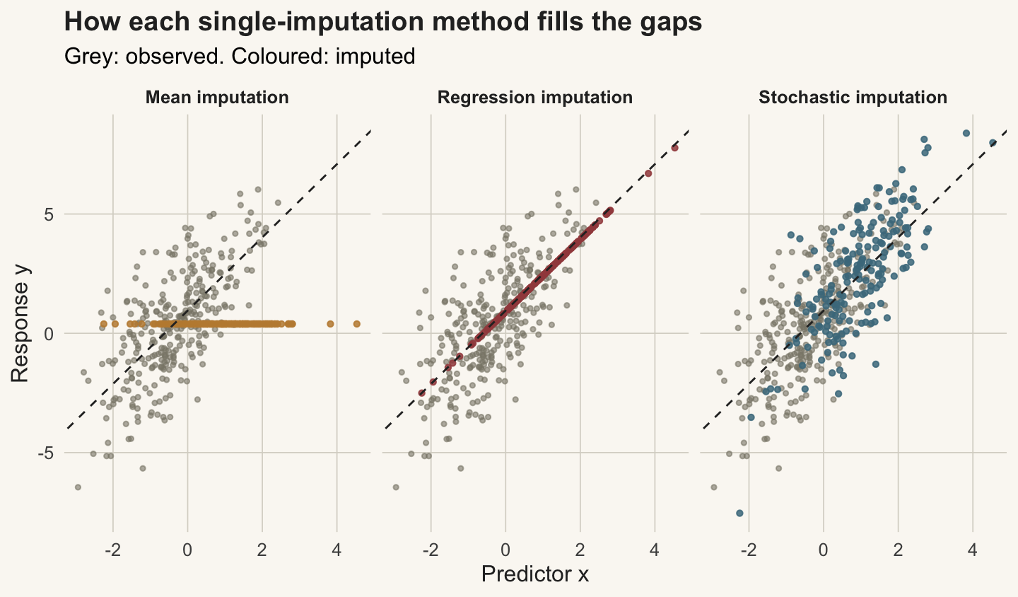
About 38% of the responses are blanked. Mean imputation replaces every gap with the observed mean of y. Regression imputation replaces each gap with its prediction from a line fitted to the complete cases. Stochastic regression imputation adds a random residual to that prediction, so the filled points scatter around the line instead of lying on it. Figure 1 shows the three fills against the observed points.

lev <- c("Mean imputation", "Regression imputation", "Stochastic imputation")
mkp <- function(yo, nm) data.frame(x = x, y = yo, nm = nm,
                                   kind = ifelse(miss, "Imputed", "Observed"))
df1 <- rbind(mkp(impute("mean"), lev[1]), mkp(impute("detreg"), lev[2]),
             mkp(impute("stoch"), lev[3]))
df1$nm <- factor(df1$nm, levels = lev)
fl <- coef(lm(y ~ x))
ggplot(df1, aes(x, y)) +
  geom_point(data = subset(df1, kind == "Observed"), colour = "#8a8578", size = 0.9, alpha = 0.6) +
  geom_point(data = subset(df1, kind == "Imputed"), aes(colour = nm), size = 1.1, alpha = 0.85) +
  geom_abline(intercept = fl[1], slope = fl[2], colour = ink, linewidth = 0.5, linetype = "dashed") +
  facet_wrap(~nm) + scale_colour_manual(values = imp_col, guide = "none") +
  labs(title = "How each single-imputation method fills the gaps",
       subtitle = "Grey: observed. Coloured: imputed",
       x = "Predictor x", y = "Response y") + theme_te()

Figure 1: The same missing responses filled three ways. Mean imputation places them in a flat horizontal band; regression imputation places them exactly on the fitted line; stochastic imputation scatters them around it. The dashed line is the full-data fit.

What the fills do to the estimate

Estimate the slope, the correlation, and the spread of y on each completed dataset.

estim <- function(yo) { ok <- !is.na(yo); f <- lm(yo[ok] ~ x[ok])
  c(slope = unname(coef(f)[2]), r = cor(x[ok], yo[ok]), sdY = sd(yo[ok])) }
set.seed(2947)
tab <- rbind(
  Full                    = estim(y),
  `Complete-case`         = { z <- y; z[miss] <- NA; estim(z) },
  `Mean imputation`       = estim(impute("mean")),
  `Regression imputation` = estim(impute("detreg")),
  `Stochastic imputation` = estim(impute("stoch")))
round(tab, 3)

                      slope     r   sdY
Full                  1.535 0.737 2.461
Complete-case         1.516 0.688 2.234
Mean imputation       0.692 0.465 1.758
Regression imputation 1.516 0.814 2.198
Stochastic imputation 1.606 0.768 2.468

The full data give a slope of 1.535, a correlation of 0.737, and a standard deviation of 2.461. Mean imputation drags all three down: the slope falls to 0.692, the correlation to 0.465, and the spread to 1.758. Piling filled values onto a single horizontal line flattens the relationship and shrinks the variance, so every association is diluted.

Regression imputation does the opposite to the correlation. Its slope, 1.516, matches the complete-case fit, but the correlation climbs to 0.814, above even the full-data value, because the imputed points sit perfectly on the line and manufacture agreement that is not in the data. Only stochastic imputation keeps the spread (2.468) and correlation (0.768) near their full-data values, because the added noise restores the scatter the other two erase.

So for an unbiased point estimate of the slope, mean imputation is out, and regression and stochastic imputation both land on the right answer. That would seem to settle it. It does not.

The uncertainty that single imputation hides

Repeat the whole process 2000 times, recording each method’s slope, its reported standard error, and whether the 95% interval covers the truth.

M <- 2000; keep <- c("cc", "mean", "detreg", "stoch")
sl <- se <- cv <- matrix(NA, M, 4, dimnames = list(NULL, keep))
set.seed(11072026)
for (i in 1:M) {
  xx <- rnorm(n, 0, sdx); yy <- c0 + c1 * xx + rnorm(n, 0, sde)
  a0i <- uniroot(function(a) mean(plogis(a + a1 * xx)) - 0.40, c(-6, 6))$root
  mi <- runif(n) < plogis(a0i + a1 * xx); ob <- !mi
  fit <- lm(yy[ob] ~ xx[ob]); sig <- summary(fit)$sigma
  yh <- coef(fit)[1] + coef(fit)[2] * xx[mi]
  comp <- list(cc = { z <- yy; z[mi] <- NA; z },
               mean = { z <- yy; z[mi] <- mean(yy[ob]); z },
               detreg = { z <- yy; z[mi] <- yh; z },
               stoch = { z <- yy; z[mi] <- yh + rnorm(sum(mi), 0, sig); z })
  for (k in keep) { z <- comp[[k]]; ok <- !is.na(z); f <- lm(z[ok] ~ xx[ok])
    b <- unname(coef(f)[2]); s <- summary(f)$coef[2, 2]
    sl[i, k] <- b; se[i, k] <- s
    cv[i, k] <- (b - 1.96 * s <= c1) & (c1 <= b + 1.96 * s) }
}
summ <- rbind(bias = colMeans(sl) - c1, emp_SD = apply(sl, 2, sd),
              mean_SE = colMeans(se), coverage = colMeans(cv))
round(summ, 3)

            cc   mean detreg stoch
bias     0.000 -0.804  0.000 0.000
emp_SD   0.087  0.065  0.087 0.096
mean_SE  0.088  0.057  0.046 0.060
coverage 0.947  0.000  0.702 0.785

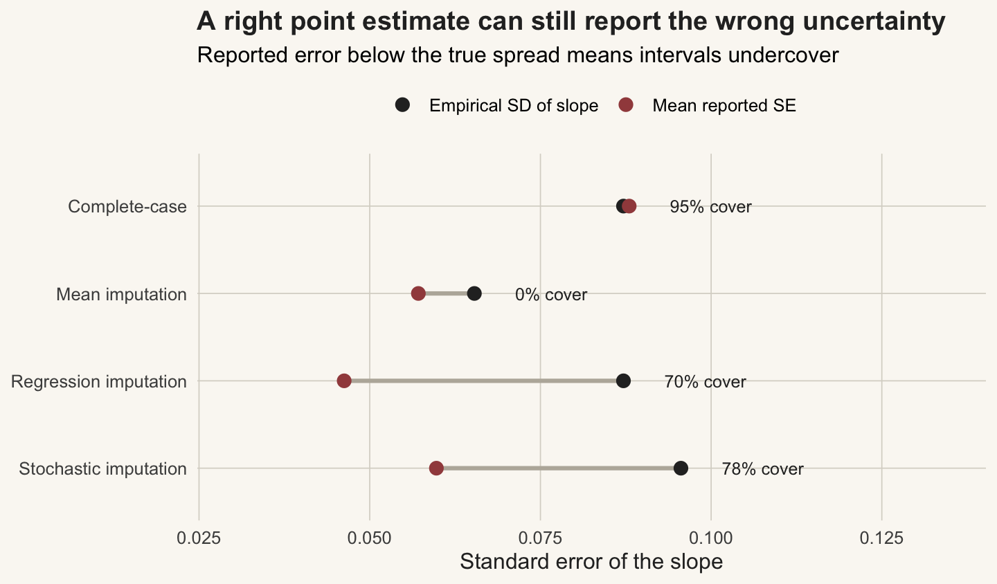
Complete-case analysis is honest: bias 0.000, and its reported error (0.088) matches the true spread of estimates (0.087), so coverage is 95%. Mean imputation fails on bias, -0.804, and never covers.

The two unbiased imputations fail on a subtler count. Regression imputation reports an average error of 0.046, roughly half the true spread of 0.087, so its intervals cover only 70% of the time. Stochastic imputation is better but not fixed: its reported error 0.06 still falls short of the true 0.096, and coverage sits at 78%. Figure 2 puts the reported error against the true spread for each method.

labs_m <- c(cc = "Complete-case", mean = "Mean imputation",
            detreg = "Regression imputation", stoch = "Stochastic imputation")
df2 <- data.frame(method = factor(labs_m, levels = rev(labs_m)),
                  emp_SD = summ["emp_SD", ], mean_SE = summ["mean_SE", ],
                  coverage = summ["coverage", ])
dfl <- pivot_longer(df2, c(emp_SD, mean_SE), names_to = "q", values_to = "v")
dfl$q <- factor(dfl$q, levels = c("emp_SD", "mean_SE"),
                labels = c("Empirical SD of slope", "Mean reported SE"))
ggplot(df2, aes(y = method)) +
  geom_segment(aes(x = mean_SE, xend = emp_SD, yend = method), colour = "#b9b4a8", linewidth = 1.1) +
  geom_point(data = dfl, aes(x = v, colour = q), size = 3) +
  geom_text(aes(x = pmax(emp_SD, mean_SE) + 0.006,
                label = sprintf("%.0f%% cover", 100 * coverage)),
            hjust = 0, size = 3.3, colour = ink) +
  scale_colour_manual(values = c("Empirical SD of slope" = "#2b2b2b", "Mean reported SE" = "#a24b4b")) +
  coord_cartesian(xlim = c(0.03, 0.135)) +
  labs(title = "A right point estimate can still report the wrong uncertainty",
       subtitle = "Reported error below the true spread means intervals undercover",
       x = "Standard error of the slope", y = NULL, colour = NULL) + theme_te()

Figure 2: Empirical spread of the slope over 2000 datasets against the average standard error each method reports, with interval coverage. Where the reported error falls short of the true spread, coverage drops below 95%.

The honest limit

Mean imputation biases the estimate; regression imputation manufactures correlation; both understate error badly. Stochastic imputation clears the bias and restores the variance, yet still reports too little uncertainty. The reason is structural, not a matter of tuning. A single completed dataset treats the filled values as if they were the true ones, so the standard error reflects only the sampling variability of that one dataset, and not the extra uncertainty from having guessed the missing values in the first place. No single imputation, however clever the fill, can express that second layer of doubt, because it commits to one set of guesses.

The fix is to stop pretending there is one right fill. Multiple imputation draws several completed datasets, analyses each, and then combines the results so that the disagreement between them feeds back into the standard error. That is the subject of the next post.

References

Little RJA, Rubin DB 2019. Statistical Analysis with Missing Data, 3rd edn. Wiley. ISBN 978-0-470-52679-8.

Enders CK 2010. Applied Missing Data Analysis. Guilford Press. ISBN 978-1-60623-639-0.

Nakagawa S, Freckleton RP 2008. Trends in Ecology and Evolution 23(11):592-596 (10.1016/j.tree.2008.06.014).

Rubin DB 1987. Multiple Imputation for Nonresponse in Surveys. Wiley. ISBN 978-0-471-08705-2.

Schafer JL 1997. Analysis of Incomplete Multivariate Data. Chapman and Hall/CRC. ISBN 978-0-412-04061-0.

Related tutorials

• Missing data: MCAR, MAR and MNAR
• Multiple imputation by chained equations
• Checking missing-data assumptions
• Checking measurement-error corrections