---
title: "Checking a stratified design"
description: "Three diagnostics for stratified survey estimates in R: post-stratification instability, weights that no longer match the frame, and far too many strata."
date: "2026-06-27 10:00"
date-modified: "2026-10-15"
categories: [R, survey design, model checking, ecology tutorial]
image: thumbnail.png
image-alt: "Single panel line chart with points: design variance drops steeply from about 0.24 at one stratum to under 0.05 by six strata, then runs flat out to thirty; one point at four strata is highlighted in red."
---
*Corrected 15 October 2026: the introduction said that in all three places the answer is still wrong, and the section on many strata said that strata beyond a handful buy almost nothing in precision; it now says the result can still mislead and that the extra strata buy much less than the first few did. The extra variance from post-stratifying a small sample is now given as the figure from this run of replicates, which moves by a few points from one run to the next.*
*Corrected 7 October 2026: the post presented the coverage slip on a small sample as a cost of post-stratifying, and said that with many strata the reported uncertainty becomes unreliable; it now says part of the slip comes with any survey that small, that what post-stratification adds is variance and unusable samples, and that coverage holds with many strata while the standard error from any one survey gets less reliable.*
*Corrected 30 September 2026: the post said more data makes a weight error worse; the mean squared error still falls with sample size while the bias stays fixed, so it now says more data does not shrink the error and makes the interval more misleading.*
The three posts before this one built stratified estimators and trusted them. This one distrusts them. A stratified survey has three places where the arithmetic is exactly right and the result can still mislead, and none of them announces itself in the standard error you report.
The first is stratifying after the fact instead of before. The second is using stratum weights that no longer describe the ground. The third is chopping the landscape into so many strata that the variance estimator falls apart while the point estimate looks fine. Each gets a demonstration on a landscape where the truth is known, so the failure is measurable rather than asserted.
## The landscape and the honest baseline
```{r frame}
set.seed(371)

Nh   <- c(meadow = 600, wetland = 300, woodland = 300)
mu_h <- c(meadow = 12,  wetland = 26,  woodland = 5)
sd_h <- c(meadow = 4,   wetland = 9,   woodland = 2)

N       <- sum(Nh)
H       <- length(Nh)
stratum <- rep(names(Nh), Nh)
y       <- round(pmax(0, rnorm(N, rep(mu_h, Nh), rep(sd_h, Nh))), 2)

W     <- Nh / N
mu    <- mean(y)
S2    <- var(y)
S2h   <- tapply(y, stratum, var)[names(Nh)]
muh   <- tapply(y, stratum, mean)[names(Nh)]
idx_h <- split(seq_len(N), stratum)[names(Nh)]

n  <- 120
nh <- round(n * W)
f  <- n / N
V_str <- sum(W^2 * (1 - nh / Nh) * S2h / nh)
V_srs <- (1 - f) * S2 / n
c(V_stratified = V_str, V_srs = V_srs)
```
## Check one: post-stratification is not free stratification
A tempting shortcut: take a simple random sample, note afterwards which stratum each plot fell in, and combine the stratum means with the known weights. You get the stratified estimator without having to control the sample. It is nearly as good, but the word *nearly* hides a real cost, because the stratum sample sizes are now random.
```{r post-strat}
post_strat <- function(nn) {
  s  <- sample.int(N, nn)
  st <- stratum[s]
  ys <- y[s]
  k  <- table(factor(st, levels = names(Nh)))
  if (any(k < 2)) return(c(NA, NA))               # a stratum with under two plots is unusable
  m <- tapply(ys, st, mean)[names(Nh)]
  v <- tapply(ys, st, var)[names(Nh)]
  c(sum(W * m), sum(W^2 * (1 - k[names(Nh)] / Nh) * v / k[names(Nh)]))
}

B <- 6000
set.seed(3741)
ps120 <- t(replicate(B, post_strat(120)))
extra <- (1 - f) / n^2 * sum((1 - W) * S2h)         # the leading penalty term

c(mc_variance = var(ps120[, 1], na.rm = TRUE),
  design_stratified = V_str,
  predicted = V_str + extra,
  mean_v_hat = mean(ps120[, 2], na.rm = TRUE),
  coverage = mean(abs(ps120[, 1] - mu) <= 1.96 * sqrt(ps120[, 2]), na.rm = TRUE))
```
```{r scalars-1}
#| echo: false
ps_v <- var(ps120[, 1], na.rm = TRUE)
ps_pen <- 100 * (ps_v / V_str - 1)
cov120 <- mean(abs(ps120[, 1] - mu) <= 1.96 * sqrt(ps120[, 2]), na.rm = TRUE)
```
At `r sprintf("%d", 120L)` plots the penalty is small: post-stratification variance `r sprintf("%.4f", ps_v)` against `r sprintf("%.4f", V_str)` for the designed survey, about `r sprintf("%.1f", ps_pen)` per cent higher, and the predicted value from the leading correction term lands right on it. Coverage is `r sprintf("%.3f", cov120)`, close enough. On a large sample, post-stratification is a fine recovery move.
Shrink the sample and the same shortcut turns fragile, because now some strata land with two or three plots and occasionally with fewer than two:
```{r post-strat-small}
set.seed(3742)
ps24 <- t(replicate(B, post_strat(24)))
nh24 <- round(24 * W)
c(mc_variance = var(ps24[, 1], na.rm = TRUE),
  design_stratified = sum(W^2 * (1 - nh24 / Nh) * S2h / nh24),
  coverage = mean(abs(ps24[, 1] - mu) <= 1.96 * sqrt(ps24[, 2]), na.rm = TRUE),
  fraction_unusable = mean(is.na(ps24[, 1])))
```
```{r scalars-2}
#| echo: false
cov24 <- mean(abs(ps24[, 1] - mu) <= 1.96 * sqrt(ps24[, 2]), na.rm = TRUE)
fail24 <- mean(is.na(ps24[, 1]))
pen24 <- 100 * (var(ps24[, 1], na.rm = TRUE) / sum(W^2 * (1 - nh24 / Nh) * S2h / nh24) - 1)
```
Coverage has slipped to `r sprintf("%.3f", cov24)`, but not all of that is the shortcut's doing: a survey this small, designed or not, estimates its stratum variances from few plots, and the normal multiplier in the interval makes no allowance for that noise. What post-stratification adds is variance, about `r sprintf("%.0f", pen24)` per cent above the designed survey in this run of replicates (a figure that moves by a few points from one run to the next), and the `r sprintf("%.1f", 100 * fail24)` per cent of samples that produced a stratum too thin to estimate a variance from at all. The diagnostic is simple: **if you post-stratified, report the realised stratum counts, and be suspicious of any stratum thinner than about five plots.** A designed survey fixes those counts in advance and never has this problem, which is the entire reason to design one.
## Check two: weights that no longer match the frame
The estimator multiplies each stratum mean by a weight from the frame. If the frame is stale, a habitat map from a decade ago, a digitised area that was never ground-truthed, the weights are wrong, and the error goes straight into the estimate as bias. Unlike variance, bias does not shrink when you add plots.
```{r weight-error}
bias_of <- function(d)                              # published weights overstate wetland by d
  sum(c(-d, d, 0) * muh)                            # taken from meadow, given to wetland

d_grid <- c(0.01, 0.02, 0.05, 0.10)
data.frame(weight_error = d_grid,
           bias = vapply(d_grid, bias_of, 0),
           bias_over_SE = abs(vapply(d_grid, bias_of, 0)) / sqrt(V_str))
```
```{r scalars-3}
#| echo: false
b05 <- bias_of(0.05)
r05 <- abs(b05) / sqrt(V_str)
```
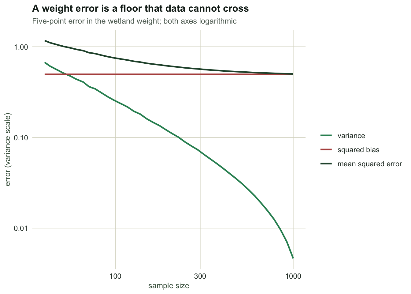
A `r sprintf("%.0f", 100 * 0.05)`-percentage-point error in the wetland weight, entirely plausible for an old map, produces a bias of `r sprintf("%.2f", b05)`, which is `r sprintf("%.2f", r05)` standard errors. The confidence interval, built from the sampling variance, has no idea this is happening: it is a tight interval around the wrong number.
The bias survives any amount of effort, and that is the point worth seeing. As the sample grows, the variance shrinks and the interval narrows onto a value that is still off:
```{r weight-mse}
mse_row <- function(nn) {
  nk <- round(nn * W)
  v  <- sum(W^2 * (1 - nk / Nh) * S2h / nk)
  b2 <- bias_of(0.05)^2
  c(n = nn, variance = v, bias_sq = b2, bias_share_of_MSE = b2 / (v + b2))
}
round(do.call(rbind, lapply(c(120, 480, 1200), mse_row)), 5)
```
```{r scalars-4}
#| echo: false
share120 <- { nk <- round(120 * W); b2 <- bias_of(0.05)^2; b2 / (sum(W^2 * (1 - nk / Nh) * S2h / nk) + b2) }
share480 <- { nk <- round(480 * W); b2 <- bias_of(0.05)^2; b2 / (sum(W^2 * (1 - nk / Nh) * S2h / nk) + b2) }
```
At `r sprintf("%d", 120L)` plots the bias is already `r sprintf("%.0f", 100 * share120)` per cent of the mean squared error; at `r sprintf("%d", 480L)` plots it is `r sprintf("%.0f", 100 * share480)` per cent. **More data does not shrink a weight error, and it makes the interval more misleading,** because it strips away the only thing that was masking the bias. The check is to age-check the frame before trusting the estimate, and, where the areas are uncertain, to carry that uncertainty through with a sweep over plausible weights rather than reporting one confident number.
```{r fig-weights}
#| echo: false
#| fig-cap: "Bias, variance and their sum against sample size, for a five-point weight error. Variance falls with effort; bias does not, so the mean squared error flattens onto the bias floor."
#| fig-alt: "Three curves against sample size on a log scale. Variance declines steeply, squared bias is flat, and total mean squared error declines then levels off at the bias line."
library(ggplot2)
theme_te <- function() {
theme_minimal(base_size = 11) +
theme(
plot.background = element_rect(fill = "#f5f4ee", colour = NA),
panel.background = element_rect(fill = "#f5f4ee", colour = NA),
panel.grid.minor = element_blank(),
panel.grid.major = element_line(colour = "#dad9ca", linewidth = 0.3),
plot.title = element_text(colour = "#16241d", face = "bold", size = 12),
plot.subtitle = element_text(colour = "#5d6b61", size = 9.5),
axis.title = element_text(colour = "#46604a", size = 9.5),
axis.text = element_text(colour = "#2c3a31", size = 9),
legend.title = element_text(colour = "#46604a", size = 9.5),
legend.text = element_text(colour = "#2c3a31", size = 9),
strip.text = element_text(colour = "#16241d", face = "bold", size = 10)
)
}
nn_grid <- round(exp(seq(log(40), log(1000), length.out = 40)))
b2 <- bias_of(0.05)^2
wd <- do.call(rbind, lapply(nn_grid, function(nn) {
nk <- round(nn * W); v <- sum(W^2 * (1 - nk / Nh) * S2h / nk)
data.frame(n = nn,
component = c("variance", "squared bias", "mean squared error"),
value = c(v, b2, v + b2))
}))
wd$component <- factor(wd$component, levels = c("variance", "squared bias", "mean squared error"))
ggplot(wd, aes(n, value, colour = component)) +
geom_line(linewidth = 0.9) +
scale_x_log10() + scale_y_log10() +
scale_colour_manual(values = c("variance" = "#2f8f63", "squared bias" = "#b5534e",
"mean squared error" = "#275139")) +
labs(title = "A weight error is a floor that data cannot cross",
subtitle = "Five-point error in the wetland weight; both axes logarithmic",
x = "sample size", y = "error (variance scale)", colour = NULL) +
theme_te()
```
## Check three: how many strata are too many
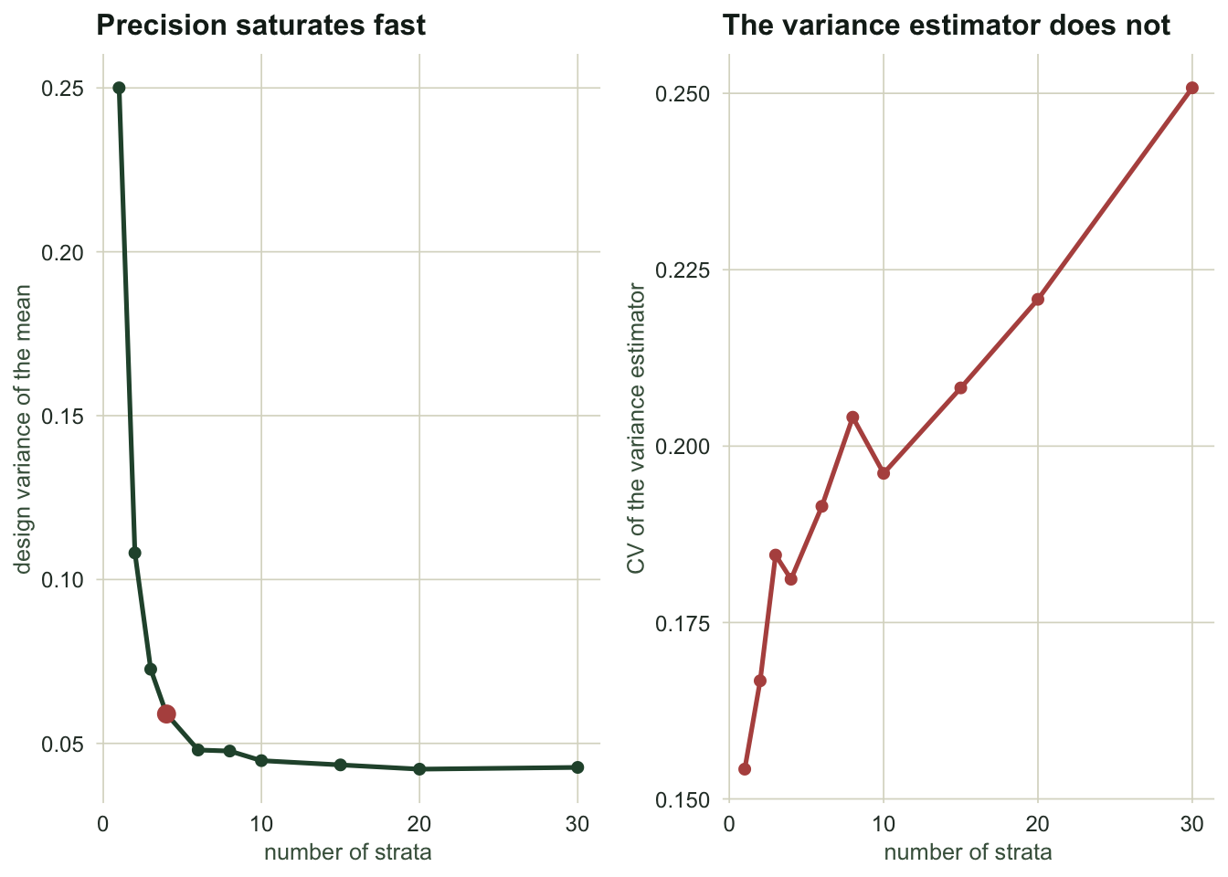
More strata remove more between-stratum variance, so the temptation is to keep splitting. Two things push back. The gain saturates quickly, and the variance estimator, which needs at least two plots per stratum, gets noisier as the plots per stratum thin out. Here is a smooth gradient sampled with a fixed 60 plots, cut into an increasing number of equal-count strata.
```{r how-many}
set.seed(3743)
M  <- 1200
x  <- sort(runif(M))
yc <- round(4 + 12 * x^2 + rnorm(M, 0, 1.6), 2)
muC <- mean(yc)
nC  <- 60
B2  <- 4000

alloc_int <- function(Wk, n) {                      # integer allocation, at least two per stratum
  a <- pmax(2, floor(n * Wk))
  while (sum(a) < n) { r <- n * Wk - a; a[which.max(r)] <- a[which.max(r)] + 1 }
  while (sum(a) > n) { r <- a - n * Wk; k <- which(a > 2); a[k[which.max(r[k])]] <- a[k[which.max(r[k])]] - 1 }
  a
}

grid <- c(1, 2, 3, 4, 6, 8, 10, 15, 20, 30)
res <- do.call(rbind, lapply(grid, function(HH) {
  g   <- cut(x, quantile(x, seq(0, 1, length.out = HH + 1)), include.lowest = TRUE, labels = FALSE)
  Nk  <- as.numeric(table(g)); Wk <- Nk / M; S2k <- as.numeric(tapply(yc, g, var))
  nk  <- alloc_int(Wk, nC)
  Vt  <- sum(Wk^2 * (1 - nk / Nk) * S2k / nk)
  ix  <- split(seq_len(M), g)
  set.seed(3744 + HH)
  rr <- t(replicate(B2, {
    s <- lapply(seq_len(HH), function(k) yc[sample(ix[[k]], nk[k])])
    c(sum(Wk * vapply(s, mean, 0)),
      sum(Wk^2 * (1 - nk / Nk) * vapply(s, var, 0) / nk))
  }))
  data.frame(H = HH, min_nh = min(nk), V_true = Vt,
             cv_v_hat = sd(rr[, 2]) / mean(rr[, 2]),
             coverage = mean(abs(rr[, 1] - muC) <= qt(0.975, sum(nk) - HH) * sqrt(rr[, 2])))
}))
round(res, 4)
```
```{r scalars-5}
#| echo: false
gain4 <- (res$V_true[res$H == 1] - res$V_true[res$H == 4]) /
(res$V_true[res$H == 1] - min(res$V_true))
cv4 <- res$cv_v_hat[res$H == 4]
cv30 <- res$cv_v_hat[res$H == 30]
```
Four strata already capture `r sprintf("%.0f", 100 * gain4)` per cent of the variance reduction that thirty strata reach. Beyond a handful the curve is nearly flat, so the extra strata buy much less than the first few did. What they cost shows up in the `cv_v_hat` column: the variance estimator's own variability climbs from `r sprintf("%.2f", cv4)` at four strata to `r sprintf("%.2f", cv30)` at thirty, because each stratum variance is now estimated from two or three plots. The point estimate stays fine throughout, and so does the coverage of the t interval in the last column; what becomes less reliable is the standard error reported by any one survey.
```{r fig-strata}
#| echo: false
#| fig-cap: "Design variance and the noise in its own estimator, against the number of strata. Precision saturates after a handful of strata while the variance estimator keeps getting noisier."
#| fig-alt: "Two panels against number of strata. The left panel shows design variance dropping steeply then flattening. The right panel shows the coefficient of variation of the variance estimator rising overall, with two small dips."
library(grid)
p_left <- ggplot(res, aes(H, V_true)) +
geom_line(colour = "#275139", linewidth = 0.9) +
geom_point(colour = "#275139", size = 1.8) +
annotate("point", x = 4, y = res$V_true[res$H == 4], colour = "#b5534e", size = 3) +
labs(title = "Precision saturates fast",
x = "number of strata", y = "design variance of the mean") +
theme_te()
p_right <- ggplot(res, aes(H, cv_v_hat)) +
geom_line(colour = "#b5534e", linewidth = 0.9) +
geom_point(colour = "#b5534e", size = 1.8) +
labs(title = "The variance estimator does not",
x = "number of strata", y = "CV of the variance estimator") +
theme_te()
grid.newpage()
pushViewport(viewport(layout = grid.layout(1, 2)))
print(p_left, vp = viewport(layout.pos.row = 1, layout.pos.col = 1))
print(p_right, vp = viewport(layout.pos.row = 1, layout.pos.col = 2))
```
Push it to the limit and the estimator stops working entirely. One plot per stratum leaves no within-stratum replication, and the variance is not estimable at all:
```{r one-per-stratum}
HH <- 60
g  <- cut(x, quantile(x, seq(0, 1, length.out = HH + 1)), include.lowest = TRUE, labels = FALSE)
Nk <- as.numeric(table(g)); Wk <- Nk / M
ix <- split(seq_len(M), g)
set.seed(3750)
s  <- lapply(seq_len(HH), function(k) yc[sample(ix[[k]], 1)])
v_hat <- sum(Wk^2 * (1 - 1 / Nk) * vapply(s, var, 0) / 1)
c(true_design_variance = sum(Wk^2 * (1 - 1 / Nk) * as.numeric(tapply(yc, g, var)) / 1),
  estimated_variance = v_hat)
```
The estimate is `NA`: with a single plot per stratum the sample variance is undefined, and no amount of cleverness recovers it from that design. The rule that falls out is unglamorous and firm: **stratify enough to catch the main structure, then stop; a stratum you cannot put two plots in is a stratum you cannot report uncertainty for.**
## The honest limit
These three diagnostics do what checks in this series always do. They catch the failure, they do not certify success. Post-stratification counts can look healthy and the estimator can still be off if the sample missed a rare stratum entirely. A frame can pass an age check and be wrong for a reason the check never asked about. And a sensible number of strata guarantees nothing if the strata were drawn along the wrong variable, so that they separate something you are not measuring while cutting across the thing you are.
The deeper limit is the one under all four posts. A design-based survey is honest about sampling and silent about everything else. It says nothing about measurement error at the plot, nothing about a frame that omits part of the population, nothing about a definition of the response that drifted between crews. Those live outside the sampling variance, which is exactly why they need their own checks rather than a wider confidence interval.
## Where to go next
That closes the stratification group: how to split a landscape, how to allocate effort across the pieces, how to build the strata when you lack a map, and how to check the result. For the spatial side of survey design, where the question is not which stratum but which locations, the companion group on spatially balanced sampling picks up the thread.
## References
Holt and Smith 1979 J R Stat Soc A 142(1):33-46 (10.2307/2344652)
Little 1993 J Am Stat Assoc 88(423):1001-1012 (10.1080/01621459.1993.10476368)
Cochran 1977 Sampling Techniques, 3rd edn, Wiley; ISBN 978-0-471-16240-7
Sarndal, Swensson and Wretman 1992 Model Assisted Survey Sampling, Springer; ISBN 978-0-387-40620-6
Lohr 2019 Sampling: Design and Analysis, 2nd edn, Chapman and Hall; ISBN 978-0-367-27950-9
## Related tutorials
- [Stratified random sampling in ecology](../stratified-random-sampling/)
- [Allocating survey effort across strata](../allocating-effort-across-strata/)
- [Multilevel post-stratification of records](../poststratifying-unstructured-records/)
- [Design weights in a stratified regression](../weights-in-a-stratified-regression/)