library(mgcv)
library(ggplot2)
library(patchwork)

te_paper  <- "#f5f4ee"
te_ink    <- "#16241d"
te_body   <- "#2c3a31"
te_forest <- "#275139"
te_rust   <- "#b5534e"
te_gold   <- "#c9b458"
te_line   <- "#dad9ca"

theme_datasheet <- function() {
  theme_minimal(base_size = 12) +
    theme(plot.background  = element_rect(fill = te_paper, colour = NA),
          panel.background = element_rect(fill = te_paper, colour = NA),
          panel.grid.major = element_line(colour = te_line, linewidth = 0.3),
          panel.grid.minor = element_blank(),
          text             = element_text(colour = te_body),
          plot.title       = element_text(colour = te_ink, face = "bold"),
          plot.subtitle    = element_text(colour = te_body),
          axis.text        = element_text(colour = te_body),
          strip.text       = element_text(colour = te_ink, face = "bold"))
}Multilevel post-stratification of records
R
mgcv
citizen science
survey design
hierarchical models
ecology tutorial
Citizen-science records leave remote cells empty. Measuring in R how raw post-stratification, a main-effects GLM and MRP in mgcv recover a frame prevalence.
A regional atlas wants one number: the share of the county’s land where a ground-nesting beetle occurs. The data are a year of citizen-science records, each one a visit to a place with a note of whether the beetle was found. The frame is well known, because the land cover map and the road network give the area of every combination of habitat and distance from a road. The records are not spread over that frame the way the land is. They pile up beside car parks and footpaths, and the far side of the moor has a handful, or none.
The survey answer to uneven coverage is post-stratification: estimate within cells of the frame, then weight the cell estimates by the known cell areas. Checking a stratified design measures what that costs when a random sample leaves a stratum thin by chance, and advises suspicion of any stratum thinner than about five plots. Non-response and site substitution post-stratifies a forest survey on a terrain covariate and finds that post-stratification pulls each of four substitution rules back towards the truth. In the first, the thin strata are thin by chance. In the second, the lost plots follow terrain, and reweighting can repair that because every terrain class still holds reached plots to stand in for the lost ones. A record stream can leave a cell with nothing to stand in, and for a reason: the empty cells are the remote ones, and remoteness is often part of why a species is there.
The regression answer to the same problem is covariate adjustment. Checking an unstructured-data analysis corrects a trend from opportunistic lists with a habitat covariate and a list-length term, and hierarchical GAMs and factor smooths shows a sparsely sampled group borrowing its shape from the others through a shared penalty. Multilevel regression and post-stratification, MRP for short, joins the two ideas: a regression with main effects plus a random effect for every cell, predicted onto the complete frame and weighted by cell area. Park, Gelman and Bafumi used it to get state estimates from national polls in which some states had almost no respondents. This post measures whether it does the same job for a record stream, against raw post-stratification and against a plain regression, with the true frame prevalence known in every replicate.
A frame, a record stream and the cells nobody visits
Every constant of the simulation sits in the next chunk and was written down before the first replicate ran; none was changed afterwards.
hab_lab   <- c("grassland", "scrub", "woodland", "wetland", "arable")
n_hab     <- length(hab_lab)
n_rem     <- 6
hab_share <- c(0.30, 0.15, 0.25, 0.10, 0.20)
rem_share <- c(0.08, 0.12, 0.16, 0.18, 0.21, 0.25)
region_km2 <- 10000

frame_cells <- expand.grid(rem = seq_len(n_rem), hab = seq_len(n_hab))
frame_cells$area <- region_km2 * hab_share[frame_cells$hab] *
  rem_share[frame_cells$rem]
frame_cells$habf <- factor(hab_lab[frame_cells$hab], levels = hab_lab)
frame_cells$cell <- factor(seq_len(nrow(frame_cells)))
n_cell  <- nrow(frame_cells)
w_frame <- frame_cells$area / sum(frame_cells$area)

b_zero    <- -1.2
hab_eff   <- c(0.4, -0.2, 0.6, -0.6, -0.8)
b_rem     <- 0.35
sd_cell   <- 0.6
slope_dev <- c(0, -0.1, 0.25, 0.35, -0.3)
decay     <- 0.7

eff_rel <- frame_cells$area * exp(-decay * (frame_cells$rem - 1))
eff_rel <- eff_rel / sum(eff_rel)

sim_cells <- function(n_rec, scen) {
  eta <- b_zero + hab_eff[frame_cells$hab] + b_rem * (frame_cells$rem - 1) +
    rnorm(n_cell, 0, sd_cell)
  if (scen == "structured") {
    eta <- eta + slope_dev[frame_cells$hab] * (frame_cells$rem - 1)
  }
  p_true <- plogis(eta)
  n_obs  <- rpois(n_cell, n_rec * eff_rel)
  list(p = p_true, n = n_obs, y = rbinom(n_cell, n_obs, p_true),
       truth = sum(w_frame * p_true))
}

rem_area_share <- tapply(w_frame, frame_cells$rem, sum)
rem_rec_share  <- tapply(eff_rel, frame_cells$rem, sum)
The frame has five habitats and six remoteness classes, thirty cells in all, over a notional region of 10000 square kilometres. Remote land is plentiful: the most remote class holds 25 per cent of the area. The beetle’s prevalence rises with remoteness on the logit scale, differs between habitats, and each cell carries its own deviation drawn fresh in every replicate from a normal distribution with standard deviation 0.6. The expected number of records in a cell is proportional to its area times a factor that falls by 0.7 on the log scale per remoteness class.
The record effort is badly out of step with the land. The most remote class holds 25 per cent of the area and receives 3.4 per cent of the records; the class beside the roads holds 8 per cent of the area and receives 36 per cent. A second truth, called structured below, adds a habitat-specific remoteness slope on top of the independent cell deviations, so that the cell interaction has a pattern a main-effects model cannot see; it is used later as a harder test.
n_example <- 100
set.seed(4620)
ex_rep <- sim_cells(n_example, "iid")
ex_empty   <- sum(ex_rep$n == 0)
ex_w_empty <- sum(w_frame[ex_rep$n == 0])
ex_p_empty <- sum((w_frame * ex_rep$p)[ex_rep$n == 0]) / ex_w_empty
ex_p_obs   <- sum((w_frame * ex_rep$p)[ex_rep$n > 0]) / (1 - ex_w_empty)
ex_rec     <- sum(ex_rep$n)
ex_thin    <- sum(ex_rep$n %in% 1:2)
One replicate at 100 expected records makes the problem visible. It produced 105 records, and 4 of the thirty cells received none. Those empty cells carry 12 per cent of the frame area, and their area-weighted true prevalence is 0.460 against 0.517 in the cells that were visited. A further 9 cells have one or two records each. In this particular draw the empty cells hold fewer beetles than the visited ones, against the average pattern measured below: the cell effects are large enough that a single year can go either way, and that is the reason for replication.
frame_plot <- data.frame(frame_cells, p = ex_rep$p, n = ex_rep$n)
frame_plot$lab <- ifelse(frame_plot$n == 0, "empty", sprintf("%.0f", frame_plot$n))
ggplot(frame_plot, aes(factor(rem), habf, fill = p)) +
  geom_tile(colour = te_paper, linewidth = 1.2) +
  geom_text(aes(label = lab, colour = n == 0), size = 4, fontface = "bold") +
  scale_fill_gradient(low = "#e9e6d3", high = te_forest, limits = c(0, 1),
                      name = "true\nprevalence") +
  scale_colour_manual(values = c(`FALSE` = te_ink, `TRUE` = te_rust), guide = "none") +
  labs(x = "remoteness class (1 = beside a road)", y = NULL,
       title = "The record stream thins out where the species is commoner",
       subtitle = "one simulated year; numbers are records per cell") +
  theme_datasheet() +
  theme(panel.grid.major = element_blank())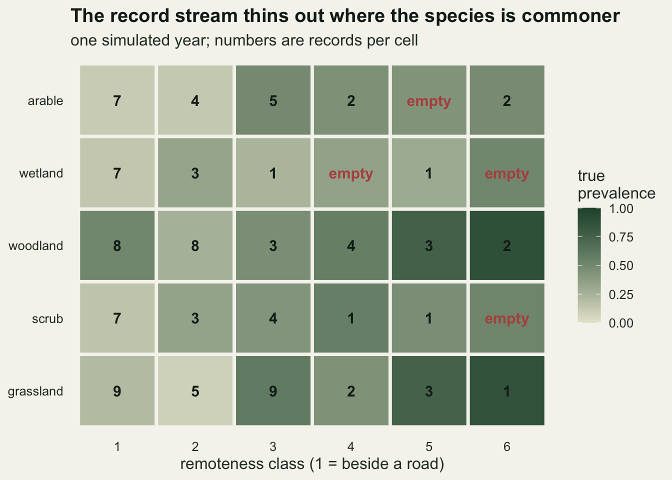
Three estimators, the same table
Every estimator below sees the same information: the number of records and the number of detections in each cell, the habitat and remoteness class of each cell, and the frame area of all thirty cells. None sees the true prevalence or the effort model. The two regressions are also given the form the truth was built with, linear in remoteness on the logit scale; the limits section returns to that.
Raw post-stratification takes the detection proportion in each visited cell and weights it by cell area. A cell with no records has no proportion, so something has to be done with it. The first version drops empty cells and rescales the remaining weights to sum to one; the second collapses each empty cell into the nearest visited cell in the same habitat, with ties going to the less remote side, so its area is kept but its prevalence is borrowed from a neighbour. Both use the stratified variance, the sum over cells of squared weight times p(1 - p) over the cell’s record count, and a normal interval. The textbook plug-in puts each cell’s own detection proportion in for p, which gives zero variance to any cell with one record, or with every record a detection or every record a miss. The intervals below put in the adjusted proportion of Agresti and Coull instead, (y + 2) / (n + 4), two detections and two misses added before dividing, so no visited cell reports zero variance; the point estimate still uses the raw proportion, and the plug-in version is kept for comparison. The variance is conditional on the realised record counts, which is the only version available when the counts were never designed.
The main-effects regression is a binomial GLM with habitat as a factor and remoteness class as a linear term on the logit scale, fitted to the visited cells, predicted onto all thirty and weighted by area. MRP is the same model plus s(cell, bs = "re"), a random intercept for every cell fitted by REML in mgcv. The factor carries all thirty levels, including the empty ones, and drop.unused.levels = FALSE keeps them in the model. For both regressions the frame estimate and its interval come from the same recipe: draw coefficient vectors from the approximate posterior (the Vp matrix that vcov() returns for a gam, and the usual covariance for the GLM), turn each draw into thirty cell prevalences, take the area-weighted sum for each draw, and report the mean and the 2.5 and 97.5 percentiles of those sums.
n_draw <- 400
x_main <- model.matrix(~ habf + rem, frame_cells)

p_adj <- function(y, n) (y + 2) / (n + 4)

ps_drop <- function(y, n) {
  keep <- n > 0
  p_c  <- y[keep] / n[keep]
  a_c  <- p_adj(y[keep], n[keep])
  w_c  <- w_frame[keep] / sum(w_frame[keep])
  est  <- sum(w_c * p_c)
  se   <- sqrt(sum(w_c^2 * a_c * (1 - a_c) / n[keep]))
  se_plug <- sqrt(sum(w_c^2 * p_c * (1 - p_c) / n[keep]))
  se_n4   <- sqrt(sum(w_c^2 * a_c * (1 - a_c) / (n[keep] + 4)))
  c(est = est, lo = est - 1.96 * se, hi = est + 1.96 * se, se = se,
    se_plug = se_plug, se_n4 = se_n4)
}

collapse_target <- function(n) {
  target <- rep(NA_integer_, n_cell)
  for (h in seq_len(n_hab)) {
    idx <- which(frame_cells$hab == h)
    has <- which(n[idx] > 0)
    if (length(has) == 0) next
    target[idx] <- idx[vapply(seq_along(idx), function(k) {
      has[which.min(abs(has - k) + 0.1 * (has > k))]
    }, 0)]
  }
  target
}

ps_collapse <- function(y, n) {
  target <- collapse_target(n)
  ok  <- !is.na(target)
  w_g <- tapply(w_frame[ok], target[ok], sum)
  y_g <- tapply(y[ok], target[ok], sum)
  n_g <- tapply(n[ok], target[ok], sum)
  w_g <- w_g / sum(w_g)
  p_g <- y_g / n_g
  a_g <- p_adj(y_g, n_g)
  est <- sum(w_g * p_g)
  se  <- sqrt(sum(w_g^2 * a_g * (1 - a_g) / n_g))
  c(est = est, lo = est - 1.96 * se, hi = est + 1.96 * se)
}

frame_summary <- function(prev_draws) {
  pop <- colSums(w_frame * prev_draws)
  c(est = mean(pop), lo = unname(quantile(pop, 0.025)),
    hi = unname(quantile(pop, 0.975)))
}

fit_glm <- function(y, n) {
  rec_tab <- data.frame(frame_cells, y = y, n = n)[n > 0, ]
  m_glm <- glm(cbind(y, n - y) ~ habf + rem, family = binomial, data = rec_tab)
  beta_sim <- rmvn(n_draw, coef(m_glm), vcov(m_glm))
  frame_summary(plogis(x_main %*% t(beta_sim)))
}

fit_mrp <- function(y, n, keep_fit = FALSE) {
  rec_tab <- data.frame(frame_cells, y = y, n = n)[n > 0, ]
  m_mrp <- gam(cbind(y, n - y) ~ habf + rem + s(cell, bs = "re"),
               family = binomial, data = rec_tab, method = "REML",
               drop.unused.levels = FALSE)
  x_frame  <- predict(m_mrp, frame_cells, type = "lpmatrix")
  beta_sim <- rmvn(n_draw, coef(m_mrp), vcov(m_mrp))
  prev_draws <- plogis(x_frame %*% t(beta_sim))
  out <- c(frame_summary(prev_draws), sd_hat = sqrt(1 / unname(m_mrp$sp[1])))
  if (keep_fit) list(summary = out, fit = m_mrp, x_frame = x_frame,
                     prev_draws = prev_draws) else out
}
The MRP interval is the part most easily got wrong, so it is checked on the example replicate before anything is repeated.
set.seed(4621)
ex_mrp <- fit_mrp(ex_rep$y, ex_rep$n, keep_fit = TRUE)
m_ex   <- ex_mrp$fit
lp_gap <- max(abs(as.vector(ex_mrp$x_frame %*% coef(m_ex)) -
                    as.vector(predict(m_ex, frame_cells, type = "link"))))
re_idx    <- grep("s(cell)", names(coef(m_ex)), fixed = TRUE)
empty_idx <- which(ex_rep$n == 0)
empty_coef <- max(abs(coef(m_ex)[re_idx][empty_idx]))
empty_sd   <- sqrt(diag(vcov(m_ex)))[re_idx][empty_idx]
vc_sd      <- unname(sqrt(m_ex$sig2 / m_ex$sp[1]))
ex_sd_hat  <- unname(ex_mrp$summary["sd_hat"])
sd_gap     <- max(abs(empty_sd - ex_sd_hat), abs(vc_sd - ex_sd_hat))
fix_idx    <- setdiff(seq_along(coef(m_ex)), re_idx)
vp_ex      <- vcov(m_ex)
block_cor  <- cov2cor(vp_ex)[fix_idx, re_idx]

beta_indep <- matrix(0, n_draw, length(coef(m_ex)))
beta_indep[, fix_idx] <- rmvn(n_draw, coef(m_ex)[fix_idx], vp_ex[fix_idx, fix_idx])
beta_indep[, re_idx]  <- rmvn(n_draw, coef(m_ex)[re_idx], vp_ex[re_idx, re_idx])
pop_indep   <- colSums(w_frame * plogis(ex_mrp$x_frame %*% t(beta_indep)))
width_full  <- unname(ex_mrp$summary["hi"] - ex_mrp$summary["lo"])
width_indep <- unname(diff(quantile(pop_indep, c(0.025, 0.975))))
cor_min     <- min(block_cor)
plug_in     <- sum(w_frame * plogis(as.vector(predict(m_ex, frame_cells, type = "link"))))

set.seed(4622)
ex_est <- rbind(drop = ps_drop(ex_rep$y, ex_rep$n)[1:3],
                collapse = ps_collapse(ex_rep$y, ex_rep$n),
                glm = fit_glm(ex_rep$y, ex_rep$n),
                mrp = ex_mrp$summary[1:3])
round(cbind(ex_est, truth = ex_rep$truth), 3)
est lo hi truth
drop 0.449 0.304 0.593 0.51
collapse 0.436 0.281 0.590 0.51
glm 0.479 0.354 0.601 0.51
mrp 0.456 0.345 0.567 0.51Three things were checked. The linear predictor matrix reproduces the model’s own predictions for all thirty cells exactly, so the draws are being pushed through the same model that was fitted. For the 4 empty cells the fitted random effect is 0.0 and its posterior standard deviation in Vp equals the REML estimate of the cell standard deviation, 2.678 (a poor estimate of the true 0.6, from one thin year), exactly; the standard deviation implied by the smoothing parameter, the square root of the scale over the smoothing parameter (the quantity gam.vcomp reports), agrees as well. An empty cell is given the population distribution of cell effects, which is the multilevel answer to having no data. Finally, the draws have to come from the joint matrix, fixed and random blocks together, because the two blocks are not independent: the most negative correlation between a fixed coefficient and a cell effect in Vp is -0.87. Drawing the two blocks separately, as if they were, gives an interval 0.418 wide against 0.222 from the joint draws.
The point estimate is the mean of the population draws, not the plug-in prevalence from the fitted coefficients, because averaging over the cell effects before the inverse logit matters: the plug-in value here is 0.445 against a simulation mean of 0.456. On this one replicate the true frame prevalence is 0.510; dropping the empty cells gives 0.449, collapsing them 0.436, the main-effects regression 0.479 and MRP 0.456. One replicate ranks nothing, which is what the next section is for.
cell_df <- data.frame(p_true = ex_rep$p,
                      mrp = rowMeans(ex_mrp$prev_draws),
                      raw = ifelse(ex_rep$n > 0, ex_rep$y / pmax(ex_rep$n, 1), NA),
                      status = ifelse(ex_rep$n == 0, "empty",
                                      ifelse(ex_rep$n <= 2, "one or two records",
                                             "three or more records")))
cell_df$status <- factor(cell_df$status,
                         levels = c("empty", "one or two records", "three or more records"))
cell_long <- rbind(
  data.frame(p_true = cell_df$p_true, estimate = cell_df$raw,
             status = cell_df$status, method = "raw cell proportion"),
  data.frame(p_true = cell_df$p_true, estimate = cell_df$mrp,
             status = cell_df$status, method = "multilevel model"))
cell_long$method <- factor(cell_long$method,
                           levels = c("raw cell proportion", "multilevel model"))
ggplot(cell_long[!is.na(cell_long$estimate), ], aes(p_true, estimate, colour = status)) +
  geom_abline(slope = 1, intercept = 0, linetype = "dashed", colour = te_body) +
  geom_point(size = 2.6, alpha = 0.9) +
  facet_wrap(~ method) +
  scale_colour_manual(values = c(te_rust, te_gold, te_forest), name = NULL, drop = FALSE) +
  coord_equal(xlim = c(0, 1), ylim = c(0, 1)) +
  labs(x = "true cell prevalence", y = "estimated cell prevalence",
       title = "Empty cells get a value only from the model",
       subtitle = "the same thirty cells; dashed line: estimate equals truth") +
  theme_datasheet() +
  theme(legend.position = "bottom")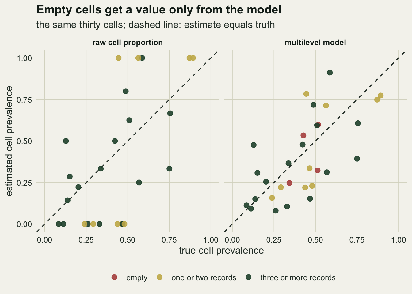
What the empty cells cost over many replicates
The loop below runs every estimator on every replicate. Each replicate draws new cell effects, new record counts and new detections, so the truth moves with the replicate and every error is measured against its own replicate’s truth.
n_rep     <- 500
cov_mcse  <- sqrt(0.95 * 0.05 / n_rep)
rec_grid  <- c(100, 300, 900)
scen_grid <- c("iid", "structured")

run_one <- function(n_rec, scen) {
  cells <- sim_cells(n_rec, scen)
  empty <- cells$n == 0
  w_e   <- sum(w_frame[empty])
  gap   <- if (any(empty)) {
    sum((w_frame * cells$p)[empty]) / w_e - sum((w_frame * cells$p)[!empty]) / (1 - w_e)
  } else 0
  n_pos <- cells$n[!empty]
  y_pos <- cells$y[!empty]
  tgt   <- collapse_target(cells$n)
  moved <- empty & !is.na(tgt)
  c(truth = cells$truth, empty = mean(empty), w_empty = w_e,
    drop_shift = -w_e * gap, gap = gap, any_empty = any(empty),
    n_empty = sum(empty), empty_far = sum(empty & frame_cells$rem >= n_rem - 1),
    degenerate = mean(y_pos == 0 | y_pos == n_pos),
    rem6_empty = all(cells$n[frame_cells$rem == n_rem] == 0),
    n_moved = sum(moved),
    moved_nearer = sum(frame_cells$rem[tgt[moved]] < frame_cells$rem[moved]),
    drop = ps_drop(cells$y, cells$n),
    collapse = ps_collapse(cells$y, cells$n),
    glm = fit_glm(cells$y, cells$n),
    mrp = fit_mrp(cells$y, cells$n))
}

time_sim <- system.time({
  sim_out <- list()
  for (s_i in seq_along(scen_grid)) for (r_i in seq_along(rec_grid)) {
    set.seed(7300 + 10 * s_i + r_i)
    sim_out[[paste(scen_grid[s_i], rec_grid[r_i])]] <-
      as.data.frame(t(replicate(n_rep, run_one(rec_grid[r_i], scen_grid[s_i]))))
  }
})
The replication was fixed at 500 replicates for each of three effort levels and both truths before the simulation ran. That gives a Monte Carlo standard error of 0.010 for a coverage near 95 per cent.
est_names <- c(drop = "post-stratified, empty cells dropped",
               collapse = "post-stratified, empty cells collapsed",
               glm = "main-effects regression",
               mrp = "multilevel regression (MRP)")
summ_tab <- do.call(rbind, lapply(names(sim_out), function(k) {
  res <- sim_out[[k]]
  do.call(rbind, lapply(names(est_names), function(e) {
    err <- res[[paste0(e, ".est")]] - res$truth
    hit <- res[[paste0(e, ".lo")]] <= res$truth & res[[paste0(e, ".hi")]] >= res$truth
    data.frame(scen = sub(" .*", "", k), n_rec = as.numeric(sub(".* ", "", k)),
               est = e, bias = mean(err), bias_se = sd(err) / sqrt(n_rep),
               rmse = sqrt(mean(err^2)), coverage = mean(hit),
               width = mean(res[[paste0(e, ".hi")]] - res[[paste0(e, ".lo")]]))
  }))
}))
get_val <- function(scen, n_rec, est, col) {
  summ_tab[summ_tab$scen == scen & summ_tab$n_rec == n_rec & summ_tab$est == est, col]
}

miss_tab <- do.call(rbind, lapply(names(sim_out), function(k) {
  res <- sim_out[[k]]
  data.frame(key = k, empty = mean(res$empty), w_empty = mean(res$w_empty),
             any_empty = mean(res$any_empty), gap = mean(res$gap[res$any_empty == 1]),
             gap_se = sd(res$gap[res$any_empty == 1]) / sqrt(sum(res$any_empty)),
             drop_shift = mean(res$drop_shift), degenerate = mean(res$degenerate),
             rem6_empty = mean(res$rem6_empty),
             far_share = sum(res$empty_far) / max(1, sum(res$n_empty)),
             sd_zero = mean(res$mrp.sd_hat < 0.05), sd_med = median(res$mrp.sd_hat),
             drop_se_mean = mean(res$drop.se_plug), drop_sd = sd(res$drop.est - res$truth),
             drop_adj_se_mean = mean(res$drop.se),
             drop_plug_cov = mean(abs(res$drop.est - res$truth) <= 1.96 * res$drop.se_plug),
             drop_n4_cov = mean(abs(res$drop.est - res$truth) <= 1.96 * res$drop.se_n4),
             nearer_share = sum(res$moved_nearer) / max(1, sum(res$n_moved)),
             sd_med_live = median(res$mrp.sd_hat[res$mrp.sd_hat >= 0.05]),
             mrp_cov_zero = mean((res$mrp.lo <= res$truth & res$mrp.hi >= res$truth)[res$mrp.sd_hat < 0.05]),
             mrp_cov_live = mean((res$mrp.lo <= res$truth & res$mrp.hi >= res$truth)[res$mrp.sd_hat >= 0.05]))
}))
plug_tab <- data.frame(scen = sub(" .*", "", miss_tab$key),
                       n_rec = as.numeric(sub(".* ", "", miss_tab$key)),
                       est = "drop_plug", coverage = miss_tab$drop_plug_cov)
rownames(miss_tab) <- miss_tab$key
show_tab <- summ_tab[, c("scen", "n_rec", "est", "bias", "rmse", "coverage")]
show_tab[, 4:6] <- round(show_tab[, 4:6], 4)
show_tab
scen n_rec est bias rmse coverage
1 iid 100 drop -0.0203 0.0779 0.956
2 iid 100 collapse -0.0198 0.0867 0.964
3 iid 100 glm 0.0055 0.0712 0.952
4 iid 100 mrp 0.0054 0.0665 0.966
5 iid 300 drop -0.0018 0.0504 0.978
6 iid 300 collapse -0.0026 0.0521 0.972
7 iid 300 glm 0.0028 0.0439 0.946
8 iid 300 mrp 0.0019 0.0415 0.964
9 iid 900 drop 0.0008 0.0287 0.960
10 iid 900 collapse 0.0008 0.0287 0.960
11 iid 900 glm -0.0002 0.0286 0.906
12 iid 900 mrp -0.0001 0.0254 0.954
13 structured 100 drop -0.0240 0.0814 0.946
14 structured 100 collapse -0.0219 0.0858 0.958
15 structured 100 glm 0.0098 0.0705 0.966
16 structured 100 mrp 0.0062 0.0666 0.976
17 structured 300 drop -0.0046 0.0471 0.976
18 structured 300 collapse -0.0038 0.0470 0.980
19 structured 300 glm 0.0026 0.0435 0.932
20 structured 300 mrp 0.0005 0.0401 0.958
21 structured 900 drop -0.0021 0.0261 0.964
22 structured 900 collapse -0.0018 0.0261 0.968
23 structured 900 glm 0.0030 0.0277 0.900
24 structured 900 mrp -0.0018 0.0233 0.952m100 <- miss_tab["iid 100", ]
m300 <- miss_tab["iid 300", ]
m900 <- miss_tab["iid 900", ]
b_drop100 <- get_val("iid", 100, "drop", "bias")
se_drop100 <- get_val("iid", 100, "drop", "bias_se")
b_coll100 <- get_val("iid", 100, "collapse", "bias")
rmse_drop100 <- get_val("iid", 100, "drop", "rmse")
bias_share100 <- b_drop100^2 / rmse_drop100^2
b_drop300 <- get_val("iid", 300, "drop", "bias")
se_drop300 <- get_val("iid", 300, "drop", "bias_se")
b_glm100 <- get_val("iid", 100, "glm", "bias")
se_glm100 <- get_val("iid", 100, "glm", "bias_se")
b_mrp100 <- get_val("iid", 100, "mrp", "bias")
se_mrp100 <- get_val("iid", 100, "mrp", "bias_se")
rmse_mrp100 <- get_val("iid", 100, "mrp", "rmse")
mrp_best <- all(vapply(split(summ_tab, paste(summ_tab$scen, summ_tab$n_rec)),
function(d) d$est[which.min(d$rmse)] == "mrp", TRUE))
cov_drop100 <- get_val("iid", 100, "drop", "coverage")
cov_drop300 <- get_val("iid", 300, "drop", "coverage")
cov_glm100 <- get_val("iid", 100, "glm", "coverage")
cov_glm900 <- get_val("iid", 900, "glm", "coverage")
cov_glms900 <- get_val("structured", 900, "glm", "coverage")
b_glms900 <- get_val("structured", 900, "glm", "bias")
se_glms900 <- get_val("structured", 900, "glm", "bias_se")
cov_mrp100 <- get_val("iid", 100, "mrp", "coverage")
cov_mrp300 <- get_val("iid", 300, "mrp", "coverage")
cov_mrp900 <- get_val("iid", 900, "mrp", "coverage")
cov_mrps100 <- get_val("structured", 100, "mrp", "coverage")
cov_mrps300 <- get_val("structured", 300, "mrp", "coverage")
cov_mrps900 <- get_val("structured", 900, "mrp", "coverage")
mrp_cov_min_z <- min((summ_tab$coverage[summ_tab$est == "mrp"] - 0.95) / cov_mcse)
mrp_cov_max_z <- max((summ_tab$coverage[summ_tab$est == "mrp"] - 0.95) / cov_mcse)
n_sim_rep <- n_rep * length(rec_grid) * length(scen_grid)
cov_drop900 <- get_val("iid", 900, "drop", "coverage")
cov_drops100 <- get_val("structured", 100, "drop", "coverage")
cov_drops300 <- get_val("structured", 300, "drop", "coverage")
cov_drops900 <- get_val("structured", 900, "drop", "coverage")
cov_coll100 <- get_val("iid", 100, "collapse", "coverage")
cov_colls100 <- get_val("structured", 100, "collapse", "coverage")
rmse_cut_max100 <- 1 - sqrt(1 - bias_share100)
w_glm900 <- get_val("iid", 900, "glm", "width")
w_mrp900 <- get_val("iid", 900, "mrp", "width")
c(mrp_best = mrp_best, mrp_cov_min_z = round(mrp_cov_min_z, 2)) mrp_best mrp_cov_min_z
1.00 0.21 First the review question that decides whether any of this is informative missingness rather than bad luck. At 100 expected records, 18.7 per cent of cells are empty in an average replicate, and they carry 21.4 per cent of the frame area. In replicates with at least one empty cell, the area-weighted true prevalence in the empty cells exceeds that in the visited cells by 0.084 (Monte Carlo standard error 0.005). At 300 records the empty share falls to 4.2 per cent, and at 900 empty cells turn up in only 4.0 per cent of replicates. The cells are empty because they are remote, and remote cells hold more beetles. Emptiness depends only on remoteness, which every regression below includes; if it also followed the cell deviation, no estimator here would recover it (see Honest limits).
That gap sets the bias of dropping empty cells almost exactly. Dropping them returns the area-weighted mean prevalence of the visited cells, so its shift from the truth is minus the empty area share times the gap, replicate by replicate. Averaged over replicates at 100 records that product is -0.0205, and the measured bias of the drop estimator is -0.0203 with a Monte Carlo standard error of 0.0034. Collapsing the empty cells into their neighbours does not help: its bias is -0.0198, because 96 per cent of the empty cells it moves borrow from a less remote neighbour, and less remote cells have a lower prevalence on average.
So raw post-stratification is biased here, as the argument says it should be. What the measurement adds is the size. At 100 records the drop estimator’s root mean squared error is 0.0779, and its bias accounts for 6.8 per cent of the mean squared error. The rest is variance from thin cells. At 300 records the bias is -0.0018, which is 0.8 standard errors from zero and not resolved by 500 replicates.
The two regressions have small positive biases at the thinnest effort, +0.0055 for the main-effects model and +0.0054 for MRP, which are 1.7 and 1.8 Monte Carlo standard errors from zero: a hint of the opposite sign, not a resolved bias. The comparison that is resolved is accuracy. MRP has the smallest root mean squared error of the four estimators at every effort level under both truths; at 100 records it is 0.0665 against 0.0779 for dropping, a reduction of 15 per cent.
plot_tab <- summ_tab
plot_tab$estimator <- factor(est_names[plot_tab$est], levels = est_names)
plot_tab$truth_lab <- ifelse(plot_tab$scen == "iid", "independent cell effects",
                             "structured interaction")
est_cols <- c(te_rust, te_gold, te_ink, te_forest)
est_lty  <- c("solid", "solid", "22", "solid")
est_shp  <- c(16, 16, 1, 16)
p_bias <- ggplot(plot_tab, aes(n_rec, bias, colour = estimator)) +
  geom_hline(yintercept = 0, colour = te_body, linewidth = 0.4) +
  geom_errorbar(aes(ymin = bias - 2 * bias_se, ymax = bias + 2 * bias_se),
                width = 0.06, linewidth = 0.5,
                position = position_dodge(width = 0.15)) +
  geom_point(aes(shape = estimator), size = 2.2, stroke = 1,
             position = position_dodge(width = 0.15)) +
  scale_shape_manual(values = est_shp, name = NULL) +
  facet_wrap(~ truth_lab) +
  scale_x_log10(breaks = rec_grid) +
  expand_limits(x = c(80, 1100)) +
  scale_colour_manual(values = est_cols, name = NULL) +
  labs(x = NULL, y = "bias", title = "Dropping empty cells is biased; the error is mostly variance",
       subtitle = "bars: two Monte Carlo standard errors") +
  theme_datasheet() +
  theme(legend.position = "none", panel.spacing.x = unit(1.5, "lines"))
p_rmse <- ggplot(plot_tab, aes(n_rec, rmse, colour = estimator)) +
  geom_line(aes(linetype = estimator), linewidth = 0.8) +
  geom_point(aes(shape = estimator), size = 2.2, stroke = 1) +
  scale_linetype_manual(values = est_lty, name = NULL) +
  scale_shape_manual(values = est_shp, name = NULL) +
  facet_wrap(~ truth_lab) +
  scale_x_log10(breaks = rec_grid) +
  expand_limits(x = c(80, 1100)) +
  scale_colour_manual(values = est_cols, name = NULL) +
  labs(x = "expected records in the year", y = "root mean squared error") +
  theme_datasheet() +
  theme(legend.position = "bottom", strip.text = element_blank(),
        panel.spacing.x = unit(1.5, "lines"), legend.key.width = unit(2, "lines")) +
  guides(colour = guide_legend(nrow = 2), linetype = guide_legend(nrow = 2),
         shape = guide_legend(nrow = 2))
(p_bias / p_rmse) + plot_annotation(theme = theme_datasheet())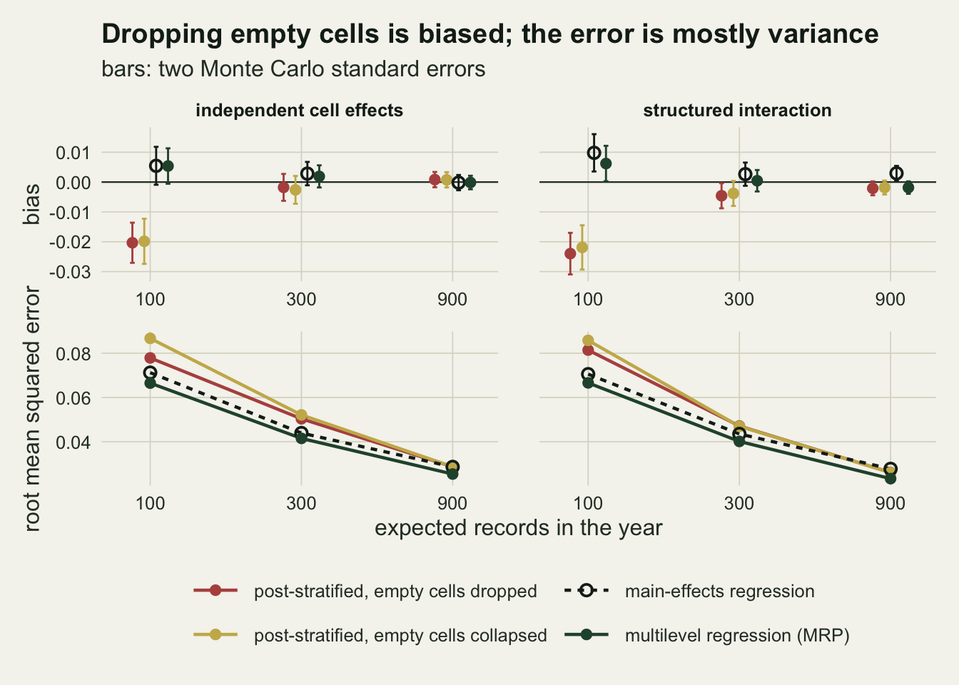
Intervals: which one can be believed
An estimator with a modest error is still unusable if its interval cannot be believed, and for raw post-stratification the variance formula decides that.
cov_band <- data.frame(lo = 0.95 - 2 * cov_mcse, hi = 0.95 + 2 * cov_mcse)
cov_names <- c(est_names, drop_plug = "dropped, plug-in variance")
cov_tab <- rbind(summ_tab[, c("scen", "n_rec", "est", "coverage")], plug_tab)
cov_tab$estimator <- factor(cov_names[cov_tab$est], levels = cov_names)
cov_tab$truth_lab <- ifelse(cov_tab$scen == "iid", "independent cell effects",
                            "structured interaction")
ggplot(cov_tab, aes(n_rec, coverage, colour = estimator)) +
  geom_rect(data = cov_band, aes(xmin = 80, xmax = 1100, ymin = lo, ymax = hi),
            inherit.aes = FALSE, fill = te_line, alpha = 0.7) +
  geom_hline(yintercept = 0.95, linetype = "dashed", colour = te_body) +
  geom_line(aes(linetype = estimator), linewidth = 0.9) +
  geom_point(aes(shape = estimator), size = 2.4, stroke = 1) +
  scale_linetype_manual(values = c(est_lty, "13"), name = NULL) +
  scale_shape_manual(values = c(est_shp, 4), name = NULL) +
  facet_wrap(~ truth_lab) +
  scale_x_log10(breaks = rec_grid) +
  scale_y_continuous(limits = c(0.5, 1), labels = function(v) sprintf("%.0f%%", 100 * v)) +
  scale_colour_manual(values = c(est_cols, te_rust), name = NULL) +
  labs(x = "expected records in the year", y = "interval coverage",
       title = "The plug-in post-stratified interval fails at thin effort",
       subtitle = "dashed: nominal 95 per cent; grey band: two Monte Carlo standard errors") +
  theme_datasheet() +
  theme(legend.position = "bottom", panel.spacing.x = unit(1.5, "lines"),
        legend.key.width = unit(2, "lines")) +
  guides(colour = guide_legend(nrow = 3), linetype = guide_legend(nrow = 3),
         shape = guide_legend(nrow = 3))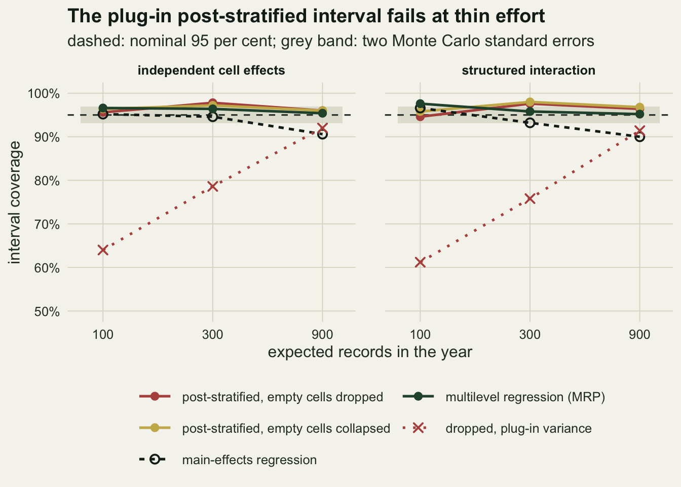
With the textbook plug-in variance, the dropped-cell interval covers the truth in 64.0 per cent of replicates at 100 records and in 78.6 per cent at 300. The bias explains little of that. The average plug-in standard error at 100 records is 0.0370 while the actual spread of the estimator around the truth is 0.0753, a ratio of 0.49. A cell with one record, or with every record a detection or every record a miss, reports a sample variance of zero, and 49 per cent of the visited cells in an average replicate are like that. This is the thin-stratum warning from the stratified design check, made far worse by a stream that never promised a minimum count per cell.
That failure belongs to the variance formula, not to post-stratification. With the adjusted proportion in the variance, the average standard error at 100 records is 0.0802, a ratio of 1.07 to the actual spread, and the same point estimates cover 95.6, 97.8 and 96.0 per cent at the three effort levels under the independent truth, and 94.6, 97.6 and 96.4 per cent under the structured truth: none clearly short any more, and at 300 records 2.9 Monte Carlo standard errors above nominal coverage. Collapsing with the same variance covers 96.4 and 95.8 per cent at 100 records. Agresti and Coull’s own interval also replaces n by n + 4 in the denominator; summed over thin cells that shrinks the standard error too far, and it covered 72.0 per cent at 100 records, so only their adjusted proportion is borrowed here.
With a sound variance, what dropping empty cells costs is the bias measured above, -0.0203 at 100 records, and it is small beside the error. It is 6.8 per cent of the mean squared error, so removing it and nothing else would lower the root mean squared error by at most 3.5 per cent; MRP’s is 15 per cent lower. The bias is also one that no interval can show, because it comes from cells nobody visited.
The main-effects regression covers well while records are scarce, 95.2 per cent at 100, and loses coverage as they accumulate: 90.6 per cent at 900 under the independent truth and 90.0 per cent under the structured one, where its bias is +0.0030 (2.4 standard errors). Its interval knows only the uncertainty in the main effects, and with enough records that shrinks below the real variation between cells that the model has no term for.
MRP covers 96.6, 96.4 and 95.4 per cent at the three effort levels under the independent truth, and 97.6, 95.8 and 95.2 per cent under the structured truth. The lowest of the six is 0.2 Monte Carlo standard errors above 95 per cent and the highest is 2.7 above it: the interval is not too short anywhere in this design, and at the thinnest effort it is a little wide.
One detail of how MRP gets there deserves a line in any report. At 100 records REML put the cell standard deviation below 0.05 in 29.0 per cent of replicates, against a true value of 0.6; at 900 it did so in 0.0 per cent. When the variance component collapses, MRP becomes the main-effects regression for that replicate, and in those replicates at 100 records its interval covered 95.2 per cent. In the remaining replicates the median REML estimate was 0.95 against 0.6, and those replicates carry the excess coverage, 97.2 per cent. The main-effects interval falls clearly short only at 900 records, and at that effort, under the independent truth, REML did not collapse the cell variance in any replicate; that is where the two regressions part company.
What to report
Report the frame before the estimate. A table of records per cell, the number of empty cells, the share of frame area they carry, and where they sit on the frame covariates tells a reader whether missing cells are a detail or the story. In this design 77.6 per cent of the empty cells at 100 records sat in the two most remote classes, and remoteness was part of the response; a reader who sees that table knows that dropping them cannot be neutral.
If raw post-stratification is used at all on a record stream, do not quote the plug-in stratified interval. It treats a cell with one record, or with all detections or all misses, as having no variance, and at 100 expected records that interval covered 64.0 per cent of the time; with the adjusted proportion in the variance the same estimates covered 95.6 per cent. Say which variance was used, and state the bias argument separately, with the empty-cell table, because the interval cannot see it. Collapsing empty cells into their neighbours is not a repair either; at the same effort it had the same bias and a larger error.
For MRP, give the model formula, the frame it was projected onto and where the frame weights came from. Say that the interval comes from joint draws of all coefficients, that each draw was turned into an area-weighted frame prevalence, and how many draws were used. Report the REML estimate of the cell standard deviation, and say plainly when it is at or near zero, because then the model is the main-effects regression and the multilevel label adds nothing for that dataset.
Put the main-effects regression beside the MRP estimate. At 900 records the main-effects interval averaged 0.0966 wide against 0.0997 for MRP, and it covered 90.6 per cent against 95.4 for MRP; a narrower interval from the simpler model is not a gain in precision. MRP’s interval also needed no variance repair: it comes straight from the fitted model.
Honest limits
The independent-cell truth is the model MRP assumes, so its good showing there is a best case. The structured truth adds one habitat-by-remoteness pattern chosen before the run, and MRP held up under it, but it is one pattern. A species found only in remote wetland, and nowhere a record could see it, is invisible to all four estimators: an empty cell gets its value from the main effects and the population of cell effects, and no amount of partial pooling reaches a deviation that exists only where nobody went.
Each record here is a visit with a clean detection or non-detection, detection is perfect, and the chance that a visit happens does not depend on whether the beetle is there. Real opportunistic records break all three. Isaac and colleagues review how uneven effort and imperfect detection enter trend estimates from such data; with imperfect detection the quantity estimated above is a reporting rate, not prevalence, and if observers go where the beetle is known to be, every estimator in this post is biased upwards.
Remoteness entered both regressions as a linear term on the logit scale, which is also how the truth was built. Entered as a factor it would have left the most remote class without an estimate whenever all five of its cells were empty, which happened in 3.8 per cent of replicates at 100 records. A curved truth fitted with a straight term would bias both regressions in the empty remote cells, and that was not measured.
The Vp matrix is conditional on the estimated smoothing parameter, which for a random effect is the cell variance (Wood 2011 describes the REML fit). The interval therefore ignores uncertainty in the cell standard deviation, and with thirty cells that uncertainty is large: REML put it near zero in 29.0 per cent of the thinnest replicates. MRP coverage held in this design anyway; a full Bayesian fit that samples the variance would carry that uncertainty, and it was not tried. The design itself is one frame of thirty cells, three effort levels and 400 posterior draws per fit; that is 3000 replicates with two regression fits each, and nothing larger was tried. The adjusted-proportion variance for post-stratification was picked after the plug-in failure had been measured, on the same design and the same replicates, so its coverage here is not an out-of-sample test of that choice.
References
Agresti A, Coull BA 1998 The American Statistician 52(2):119-126 (10.1080/00031305.1998.10480550)
Isaac NJB, van Strien AJ, August TA, de Zeeuw MP, Roy DB 2014 Methods in Ecology and Evolution 5(10):1052-1060 (10.1111/2041-210X.12254)
Park DK, Gelman A, Bafumi J 2004 Political Analysis 12(4):375-385 (10.1093/pan/mph024)
Wood SN 2011 Journal of the Royal Statistical Society Series B 73(1):3-36 (10.1111/j.1467-9868.2010.00749.x)