---
title: "Allocating survey effort across strata"
description: "Equal, proportional, Neyman and cost-aware allocation in R: which strata deserve more plots, what the optimum is worth, and how much a noisy pilot costs you."
date: "2026-06-26 14:00"
date-modified: "2026-10-15"
categories: [R, survey design, sampling, ecology tutorial]
image: thumbnail.png
image-alt: "Grouped bar chart of plots allocated to three strata under three allocation rules on the x axis (equal, proportional, Neyman); equal gives 40 plots each, proportional gives 60, 30 and 30 including the tallest bar in the figure, and Neyman is the most uneven at 52, 56 and 12."
---
*Corrected 15 October 2026: the text on the ten-plot pilot presented its comfortable result as a general rule, that the optimum is worth chasing because a near miss costs little; it now adds that the gain is large here because the stratum standard deviations differ widely, and that where the strata are about equally variable a pilot-based allocation can do worse than following area. The title of the pilot figure now says the result holds here, and the alt text of the budget figure now says Neyman sits only slightly below proportional rather than close behind the cost-aware rule.*
Once the landscape is split into strata, a second decision arrives: how many plots go where. Splitting the effort in proportion to stratum area is the obvious answer and it is a decent one, but it ignores something you often know. Some strata are far more variable than others, and a mean from a quiet stratum is already precise after a handful of plots while a noisy stratum is still wandering after twenty.
There is an exact answer to this, published by Neyman in 1934, and it is short: **send effort where the variability is, not where the area is.** This post derives it, measures what it is worth, adds field costs, and then asks the uncomfortable question of where the stratum variabilities are supposed to come from before the survey has happened.
## The same landscape as before
```{r frame}
set.seed(371)

Nh   <- c(meadow = 600, wetland = 300, woodland = 300)
mu_h <- c(meadow = 12,  wetland = 26,  woodland = 5)
sd_h <- c(meadow = 4,   wetland = 9,   woodland = 2)

N       <- sum(Nh)
H       <- length(Nh)
stratum <- rep(names(Nh), Nh)
y       <- round(pmax(0, rnorm(N, rep(mu_h, Nh), rep(sd_h, Nh))), 2)

W   <- Nh / N
S2h <- tapply(y, stratum, var)[names(Nh)]
Sh  <- sqrt(S2h)
round(rbind(weight = W, sd = Sh), 3)
```
The design variance of the stratified mean is the same expression as before, and it is now a function of the allocation vector rather than a fixed number:
```{r vstr}
V_str <- function(nh) sum(W^2 * (1 - nh / Nh) * S2h / nh)
n <- 120
```
## Four ways to split 120 plots
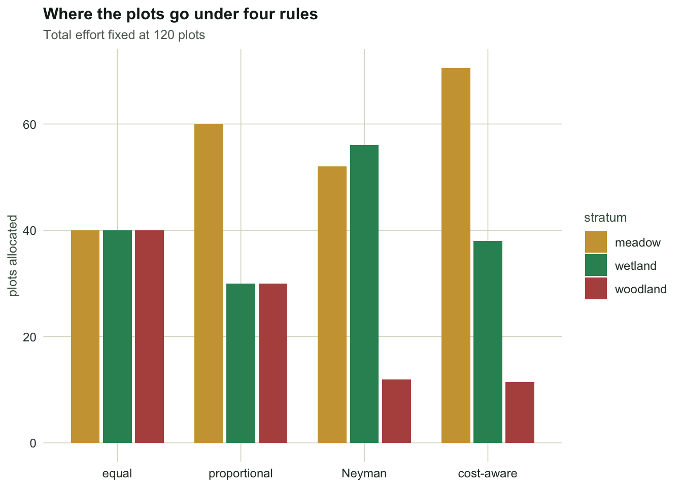
Equal allocation gives every stratum the same number of plots. Proportional allocation follows area. **Neyman allocation** follows area times standard deviation, $n_h \propto N_h S_h$. The cost-aware version divides by the square root of the per-plot cost, $n_h \propto N_h S_h / \sqrt{c_h}$, because a plot in a stratum you reach by wading is not the same purchase as a plot beside the track.
```{r allocations}
cost <- c(meadow = 1, wetland = 4, woodland = 2)     # relative cost of one plot

alloc <- list(
  equal        = setNames(rep(n / H, H), names(Nh)),
  proportional = n * W,
  Neyman       = n * W * Sh / sum(W * Sh),
  `cost-aware` = n * (W * Sh / sqrt(cost)) / sum(W * Sh / sqrt(cost)))

tab <- t(sapply(alloc, function(a)
  c(round(a, 1), SE = sqrt(V_str(a)), field_cost = sum(a * cost))))
round(tab, 3)
```
```{r scalars-1}
#| echo: false
se_eq <- sqrt(V_str(alloc$equal))
se_pr <- sqrt(V_str(alloc$proportional))
se_ne <- sqrt(V_str(alloc$Neyman))
n_ney <- alloc$Neyman
cost_pr <- sum(alloc$proportional * cost)
cost_ne <- sum(alloc$Neyman * cost)
```
Neyman sends `r sprintf("%.0f", n_ney[["wetland"]])` plots into the wetland, which is a quarter of the landscape, and only `r sprintf("%.0f", n_ney[["woodland"]])` into the woodland, which is also a quarter of it. The woodland is nearly uniform, so a dozen plots pin its mean down; the wetland is where the uncertainty lives. The standard error drops from `r sprintf("%.3f", se_pr)` under proportional allocation to `r sprintf("%.3f", se_ne)`.
```{r fig-alloc}
#| echo: false
#| fig-cap: "How four allocation rules split 120 plots. Neyman moves effort out of the uniform woodland and into the variable wetland; the cost-aware version pulls some of it back, because wetland plots are expensive."
#| fig-alt: "Grouped bar chart of plots per stratum under equal, proportional, Neyman and cost-aware allocation. Neyman gives the wetland the most plots and the woodland the fewest."
library(ggplot2)
theme_te <- function() {
theme_minimal(base_size = 11) +
theme(
plot.background = element_rect(fill = "#f5f4ee", colour = NA),
panel.background = element_rect(fill = "#f5f4ee", colour = NA),
panel.grid.minor = element_blank(),
panel.grid.major = element_line(colour = "#dad9ca", linewidth = 0.3),
plot.title = element_text(colour = "#16241d", face = "bold", size = 12),
plot.subtitle = element_text(colour = "#5d6b61", size = 9.5),
axis.title = element_text(colour = "#46604a", size = 9.5),
axis.text = element_text(colour = "#2c3a31", size = 9),
legend.title = element_text(colour = "#46604a", size = 9.5),
legend.text = element_text(colour = "#2c3a31", size = 9),
strip.text = element_text(colour = "#16241d", face = "bold", size = 10)
)
}
pal_h <- c(meadow = "#cda23f", wetland = "#2f8f63", woodland = "#b5534e")
ad <- do.call(rbind, lapply(names(alloc), function(a)
data.frame(rule = a, stratum = names(Nh), plots = as.numeric(alloc[[a]]))))
ad$rule <- factor(ad$rule, levels = names(alloc))
ad$stratum <- factor(ad$stratum, levels = names(Nh))
ggplot(ad, aes(rule, plots, fill = stratum)) +
geom_col(position = position_dodge(width = 0.78), width = 0.7) +
scale_fill_manual(values = pal_h) +
labs(title = "Where the plots go under four rules",
subtitle = "Total effort fixed at 120 plots",
x = NULL, y = "plots allocated") +
theme_te()
```
## What Neyman is worth, exactly
Drop the finite population correction for a moment and the two variances have clean closed forms: proportional allocation gives $\sum_h W_h S_h^2 / n$ and Neyman gives $(\sum_h W_h S_h)^2 / n$. The gap between them is therefore a weighted variance of the stratum standard deviations:
$$V_{\text{prop}} - V_{\text{Neyman}} = \frac{1}{n}\left[\sum_h W_h S_h^2 - \Big(\sum_h W_h S_h\Big)^2\right] = \frac{\operatorname{Var}_W(S_h)}{n}.$$
```{r neyman-identity}
V_prop_nofpc   <- sum(W * S2h) / n
V_neyman_nofpc <- (sum(W * Sh))^2 / n
var_W_Sh       <- (sum(W * S2h) - (sum(W * Sh))^2) / n

c(gap = V_prop_nofpc - V_neyman_nofpc, varW = var_W_Sh,
  difference = (V_prop_nofpc - V_neyman_nofpc) - var_W_Sh)
```
```{r scalars-2}
#| echo: false
id_gap <- abs((V_prop_nofpc - V_neyman_nofpc) - var_W_Sh)
```
The identity holds to within floating-point rounding (the `difference` printed above), and it is the useful sentence of this post: **Neyman beats proportional allocation by exactly the spread of the stratum standard deviations.** If the strata are equally variable, that spread is zero and the two allocations coincide. It is not a small print caveat, it is the entire mechanism. Strata chosen to separate the mean give you the gain in the previous post; strata that differ in variability give you this one, and the two are separate properties of the same partition.
## The comparison that is actually fair
Neyman looks better than proportional in the table above, but look at the field cost column: it spent `r sprintf("%.0f", cost_ne)` cost units against `r sprintf("%.0f", cost_pr)`, because it bought expensive wetland plots. Comparing designs at equal $n$ flatters whichever design likes the expensive stratum. Fix the budget instead and let $n$ float.
```{r equal-budget}
budget <- 300
to_budget <- function(share) {                       # scale shares to exhaust the budget
  p <- share / sum(share)
  p * budget / sum(p * cost)
}

schemes <- list(proportional = W, Neyman = W * Sh, `cost-aware` = W * Sh / sqrt(cost))
bud <- t(sapply(schemes, function(s) {
  a <- to_budget(s)
  c(round(a, 1), n = sum(a), SE = sqrt(V_str(a)), spent = sum(a * cost))
}))
round(bud, 3)
```
```{r scalars-3}
#| echo: false
se_b_pr <- bud["proportional", "SE"]
se_b_ne <- bud["Neyman", "SE"]
se_b_co <- bud["cost-aware", "SE"]
n_b_pr <- bud["proportional", "n"]
n_b_co <- bud["cost-aware", "n"]
```
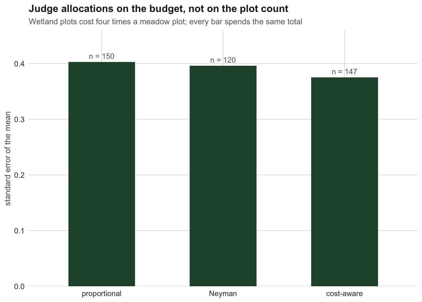
At an equal budget the ranking changes. Proportional allocation buys `r sprintf("%.0f", n_b_pr)` plots for the same money and reaches a standard error of `r sprintf("%.3f", se_b_pr)`; plain Neyman reaches `r sprintf("%.3f", se_b_ne)`, a much thinner margin than the fixed-$n$ table suggested. The cost-aware rule reaches `r sprintf("%.3f", se_b_co)` with `r sprintf("%.0f", n_b_co)` plots. Ignoring cost does not make Neyman wrong, it makes the comparison wrong.
```{r fig-budget}
#| echo: false
#| fig-cap: "Standard error achieved by three allocation rules on an identical field budget. The cost-aware rule wins because it buys more of the cheap strata and still concentrates on the variable one."
#| fig-alt: "Bar chart of standard error for proportional, Neyman and cost-aware allocation at equal budget. Cost-aware is lowest; Neyman is only slightly below proportional, which is highest."
bd <- data.frame(rule = factor(rownames(bud), levels = rownames(bud)),
SE = bud[, "SE"], n = bud[, "n"])
ggplot(bd, aes(rule, SE)) +
geom_col(fill = "#275139", width = 0.55) +
geom_text(aes(label = sprintf("n = %.0f", n)), vjust = -0.6,
colour = "#5d6b61", size = 3.2) +
scale_y_continuous(expand = expansion(mult = c(0, 0.14))) +
labs(title = "Judge allocations on the budget, not on the plot count",
subtitle = "Wetland plots cost four times a meadow plot; every bar spends the same total",
x = NULL, y = "standard error of the mean") +
theme_te()
```
## Neyman needs numbers you do not have yet
The awkward part: $S_h$ is a property of the population, and allocation happens before the survey. In practice the standard deviations come from a pilot, or from last year, or from a comparable site. A pilot of ten plots per stratum gives a noisy $\hat S_h$, and the allocation inherits the noise. Does the gain survive?
```{r pilot}
idx_h <- split(seq_len(N), stratum)[names(Nh)]
m <- 10                                              # pilot plots per stratum
B <- 2000

set.seed(3721)
V_pilot <- replicate(B, {
  sh <- vapply(idx_h, function(ix) sd(y[sample(ix, m)]), 0)
  a  <- n * W * sh / sum(W * sh)
  a  <- pmax(a, 2); a <- a * n / sum(a)              # never fewer than two plots
  V_str(a)
})

V_oracle <- V_str(alloc$Neyman)
V_propn  <- V_str(alloc$proportional)
c(median_pilot = median(V_pilot), oracle = V_oracle, proportional = V_propn,
  worse_than_proportional = mean(V_pilot > V_propn),
  gain_kept = (V_propn - median(V_pilot)) / (V_propn - V_oracle))
```
```{r scalars-4}
#| echo: false
kept <- (V_propn - median(V_pilot)) / (V_propn - V_oracle)
worse <- mean(V_pilot > V_propn)
sd_rel <- sd(V_pilot) / median(V_pilot)
```
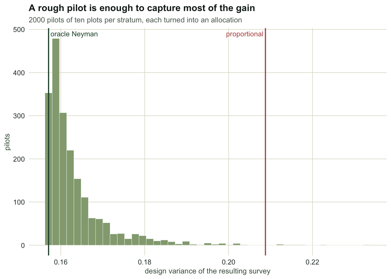
A ten-plot pilot keeps `r sprintf("%.0f", 100 * kept)` per cent of the available gain, and only `r sprintf("%.1f", 100 * worse)` per cent of pilots produce an allocation worse than simply following area. That is a more comfortable answer than it might have been, and it has two reasons: the variance is flat near its optimum, so a moderately wrong allocation costs very little, and in this landscape the gain is large, because the stratum standard deviations differ widely. Only the first reason carries over to every landscape. Where the strata are about equally variable, the gain shrinks towards zero while a noisy pilot still misallocates, and with equal standard deviations proportional allocation is itself the optimum, so any pilot-based allocation that departs from it does worse. The optimum is worth chasing when the strata clearly differ in variability, as they do here.
```{r fig-pilot}
#| echo: false
#| fig-cap: "Design variance achieved by Neyman allocations planned from a ten-plot pilot, over 2000 pilots. Almost every one lands between the oracle allocation and proportional allocation."
#| fig-alt: "Histogram of realised design variance from pilot-based allocations, with vertical lines for the oracle Neyman variance on the left and the proportional variance on the right."
ggplot(data.frame(v = V_pilot), aes(v)) +
geom_histogram(bins = 45, fill = "#93a87f", colour = "white", linewidth = 0.15) +
geom_vline(xintercept = V_oracle, colour = "#275139", linewidth = 0.7) +
geom_vline(xintercept = V_propn, colour = "#b5534e", linewidth = 0.7) +
annotate("text", x = V_oracle, y = Inf, label = " oracle Neyman", hjust = 0, vjust = 1.6,
colour = "#275139", size = 3.2) +
annotate("text", x = V_propn, y = Inf, label = "proportional ", hjust = 1, vjust = 1.6,
colour = "#b5534e", size = 3.2) +
labs(title = "Here a rough pilot captures most of the gain",
subtitle = "2000 pilots of ten plots per stratum, each turned into an allocation",
x = "design variance of the resulting survey", y = "pilots") +
theme_te()
```
## The honest limit: one allocation, several responses
The optimum is optimal for one variable. Add a second response with a different variability profile and the two optima pull in opposite directions. Here is a ground beetle count that is scarce and even in the wetland but patchy in the woodland, the reverse of the biomass pattern:
```{r second-response}
set.seed(3722)
z_mu <- c(meadow = 3,   wetland = 1.5, woodland = 6)
z_sd <- c(meadow = 1.2, wetland = 0.8, woodland = 4.5)
z    <- round(pmax(0, rnorm(N, rep(z_mu, Nh), rep(z_sd, Nh))), 2)

S2hz <- tapply(z, stratum, var)[names(Nh)]
Shz  <- sqrt(S2hz)
V_z  <- function(nh) sum(W^2 * (1 - nh / Nh) * S2hz / nh)
neyman_z <- n * W * Shz / sum(W * Shz)

rbind(sd_biomass = Sh, sd_beetles = Shz,
      `Neyman for biomass` = alloc$Neyman, `Neyman for beetles` = neyman_z)
c(beetle_V_under_biomass_plan = V_z(alloc$Neyman),
  beetle_V_under_own_plan     = V_z(neyman_z),
  beetle_V_under_proportional = V_z(alloc$proportional))
```
```{r scalars-5}
#| echo: false
z_pen_own <- V_z(alloc$Neyman) / V_z(neyman_z)
z_pen_prop <- V_z(alloc$Neyman) / V_z(alloc$proportional)
```
The allocation that is optimal for biomass is `r sprintf("%.1f", z_pen_own)` times worse than the beetle optimum, and, more to the point, `r sprintf("%.1f", z_pen_prop)` times worse than plain proportional allocation for the beetles. Optimising hard for one response can leave a second response worse off than making no attempt at all. For a multi-purpose survey, proportional allocation is the safer default; a compromise allocation, weighted across the responses that matter, is the honest middle path, and it is optimal for none of them.
Two smaller limits are worth naming. Neyman allocation can hand a stratum more plots than it contains, $n_h > N_h$, when a small stratum is very variable; in that case you census it and re-optimise over the rest. And every stratum needs at least two plots or its variance is not estimable, which quietly puts a floor under the whole exercise.
## Where to go next
Both posts so far assumed the map: known stratum sizes, known stratum membership for every plot. Field surveys frequently start without one. The next post takes a large cheap first phase to build the strata, a small expensive second phase to measure the response, and works out how to split a budget between the two.
## References
Neyman 1934 Journal of the Royal Statistical Society 97(4):558-625 (10.2307/2342192)
Tschuprow 1923 Metron 2:461-493
Cochran 1977 Sampling Techniques, 3rd edn, Wiley; ISBN 978-0-471-16240-7
Sarndal, Swensson and Wretman 1992 Model Assisted Survey Sampling, Springer; ISBN 978-0-387-40620-6
Gregoire and Valentine 2008 Sampling Strategies for Natural Resources and the Environment, Chapman and Hall; ISBN 978-1-58488-370-8
## Related tutorials
- [Stratified random sampling in ecology](../stratified-random-sampling/)
- [Two-phase sampling when strata are unknown](../two-phase-sampling-for-stratification/)
- [Checking a stratified design](../checking-a-stratified-design/)
- [Adaptive second-phase tows and the low mean](../adaptive-second-phase-tows/)