library(ggplot2)
library(patchwork)

te_paper  <- "#f5f4ee"
te_ink    <- "#16241d"
te_body   <- "#2c3a31"
te_forest <- "#275139"
te_rust   <- "#b5534e"
te_gold   <- "#c9b458"
te_line   <- "#dad9ca"

theme_datasheet <- function() {
  theme_minimal(base_size = 12) +
    theme(plot.background  = element_rect(fill = te_paper, colour = NA),
          panel.background = element_rect(fill = te_paper, colour = NA),
          panel.grid.major = element_line(colour = te_line, linewidth = 0.3),
          panel.grid.minor = element_blank(),
          text             = element_text(colour = te_body),
          plot.title       = element_text(colour = te_ink, face = "bold"),
          plot.subtitle    = element_text(colour = te_body),
          axis.text        = element_text(colour = te_body))
}Adaptive second-phase tows and the low mean
R
survey design
stratified sampling
adaptive sampling
fisheries
simulation
ecology tutorial
Sending second-phase trawl tows where phase-1 variance looks high biases the pooled stratified mean low. In R: why, by how much, and what allocation repairs it.
A research vessel has a week to survey a demersal fish on a shelf split into four depth strata. The plan is a stratified random trawl survey, but nobody knows in advance which stratum will be patchy this year, so the week is split in two. In phase 1 every stratum gets the same small number of tows. In phase 2 the remaining tows are sent out one at a time, each to the stratum where one more tow cuts the variance of the stratified mean the most, judged from the catches of phase 1. At the end the catches of both phases are pooled in each stratum and the usual stratified mean and standard error are reported.
The two-phase design is Francis (1984), written for New Zealand trawl surveys, and the same idea was used to move acoustic transects between strata during a survey of South African anchovy (Jolly and Hampton 1990). Francis’s simulations on real survey data found that it reduces the skew of the biomass estimate, and with it the chance of a gross overestimate, as well as the expected error. Surveys that use it commonly compute the gain from the squared phase-1 mean of each stratum, which stands in for the variance under a constant coefficient of variation; the post runs the rule in its variance form, with the phase-1 sample variance, and checks the mean-squared form alongside. The price is known. Once the phase-2 sizes depend on the phase-1 catches, the conventional stratified mean is no longer a design-unbiased estimator. Manly (2004), working with an extension of the Francis design to several species and locations, names bias in the estimators of totals and means as a potential problem of the method and finds that a bootstrap correction removes about half of it. A line of work on adaptive allocation builds designs and estimators to get around the problem; Moradi and Salehi (2010) went as far as constructing an adaptive allocation scheme under which the conventional estimator becomes appropriate again. The general fact that an estimate read at a data-dependent stopping point is biased is older still (Whitehead 1986). So nothing here is a discovery. What the post measures is the direction and size of the bias when most of the tows are in phase 1, what it does to the interval, where in the pooled mean it lives, and which of the obvious repairs remove it.
Four posts on this site sit next to this one. Allocating survey effort across strata plans a Neyman allocation from a pilot, notes that the standard deviations “come from a pilot, or from last year, or from a comparable site”, and measures only how good the resulting plan is: its pilot is a separate draw and is never averaged into the estimate. Here the pilot is the survey’s own first phase, and it is averaged into the answer. Adaptive cluster sampling in R adds effort where the values are high, so its naive mean runs high, and repairs it with inclusion weights. Adaptive allocation adds effort where the variance looks high; the bias has the opposite sign, and the repair turns out to be keeping the allocation from reading the data it will be averaged with. Testing a monitoring series every year is the same family seen from a trend test: stopping at the first significant look “selects for extreme estimates”. There the stopping rule reads an estimate and decides when to stop; here the rule reads a variance and decides which stratum the next tow goes to. Two-phase sampling when strata are unknown uses a first phase to build the strata and measures the response only in phase two, so no allocation there ever reads the response.
A trawl survey with four strata
The shelf has four strata covering 40, 30, 20 and 10 per cent of the area, with true mean catches of 5, 20, 60 and 150 fish per tow, so the true stratified mean is 35 fish per tow. Catches are negative binomial with size k; smaller k means more clumped catches, and three values are run, 0.6, 1 and 2. The functions below are the whole machinery: the greedy Francis rule, the stratified mean with its textbook standard error (Cochran 1977), and a Taylor power law fitted across the four strata of a survey, which is one of the repairs tested later.
W_h    <- c(0.4, 0.3, 0.2, 0.1)     # stratum area weights
mu_h   <- c(5, 20, 60, 150)         # true mean catch per tow
H      <- 4
truth  <- sum(W_h * mu_h)           # true stratified mean per tow
n_surv <- 10000                     # simulated surveys per cell
g_min  <- 2                         # floor for one-shot allocations, and guaranteed phase-2 tows
mu_moved <- c(5, 20, 150, 60)       # last year's stratum means when the stock has moved

# round a vector of sizes to integers that add to total, never below low
round_to_total <- function(x, total, low = 1) {
  base <- pmax(low, floor(x))
  left <- total - sum(base)
  if (left > 0) {
    rem <- x - floor(x)
    rem[base > floor(x)] <- -Inf
    add <- order(rem, decreasing = TRUE)[seq_len(left)]
    base[add] <- base[add] + 1
  }
  base
}

# Francis (1984) rule, variance form: each extra tow goes to the stratum with
# the largest gain W^2 v (1/n - 1/(n + 1)), one tow at a time; v is surveys x
# strata (a variance, or the squared mean in the mean-squared form)
francis <- function(v, n_start, extra) {
  n_now <- n_start
  if (extra > 0) for (s in seq_len(extra)) {
    gain <- sweep(v * (1 / n_now - 1 / (n_now + 1)), 2, W_h^2, "*")
    j    <- max.col(gain, ties.method = "first")
    idx  <- cbind(seq_len(nrow(v)), j)
    n_now[idx] <- n_now[idx] + 1
  }
  n_now
}

# stratified mean and its usual SE from tows first..last of each stratum
strat_est <- function(Y, first, last) {
  est <- 0; v_est <- 0
  for (h in 1:H) {
    tow    <- col(Y[, , h])
    keep   <- tow >= first[, h] & tow <= last[, h]
    n_used <- last[, h] - first[, h] + 1
    yy     <- Y[, , h] * keep
    m_h    <- rowSums(yy) / n_used
    s2_h   <- (rowSums(yy^2) - n_used * m_h^2) / (n_used - 1)
    est    <- est + W_h[h] * m_h
    v_est  <- v_est + W_h[h]^2 * s2_h / n_used
  }
  cbind(est = est, se = sqrt(v_est))
}

# Taylor's power law fitted across the four strata of each survey,
# by closed-form least squares on log mean and log variance
taylor_var <- function(m1, s2) {
  ok   <- m1 > 0 & s2 > 0
  lx   <- ifelse(ok, log(pmax(m1, 1e-12)), 0)
  ly   <- ifelse(ok, log(pmax(s2, 1e-12)), 0)
  n_ok <- rowSums(ok)
  xb   <- rowSums(lx * ok) / pmax(n_ok, 1)
  yb   <- rowSums(ly * ok) / pmax(n_ok, 1)
  sxx  <- rowSums(ok * (lx - xb)^2)
  sxy  <- rowSums(ok * (lx - xb) * (ly - yb))
  slope <- sxy / sxx
  fit  <- exp(yb - slope * xb) * pmax(m1, 1e-3)^slope
  bad  <- n_ok < 2 | !is.finite(slope) | sxx < 1e-12
  fit[bad, ] <- pmax(m1[bad, , drop = FALSE], 1e-3)
  fit
}

summ <- function(r) {
  rel <- r[, "est"] / truth - 1
  c(bias = mean(rel), bias_mcse = sd(rel) / sqrt(nrow(r)),
    rmse = sqrt(mean(rel^2)),
    se_ratio = mean(r[, "se"]) / sd(r[, "est"]),
    cover = mean(abs(r[, "est"] - truth) <= 1.96 * r[, "se"]))
}
Each simulated survey below draws its tows in order, so the first n1 tows of every stratum are phase 1 and the rest are available to phase 2. The same tows are then read under every allocation, which makes the arms paired. There are nine arms. The adaptive arm is the rule as run here: Francis on the phase-1 variances, both phases pooled. The fixed arm uses the adaptive arm’s own average final sizes, rounded, set before the survey. It is a yardstick, not a field option, because nobody knows those sizes in advance; it answers what the same allocation would do if it did not read the data. Neyman on the true standard deviations and proportional allocation spend the same total in one shot. The last-year arm runs the Francis rule on the variances of an independent earlier survey with n1 tows per stratum, the size of this year’s phase 1, and a second version does so after the dense patch has moved from the deepest stratum to the one above it. The Taylor arm allocates from the fitted power law. The last two arms guarantee 2 phase-2 tows in every stratum, send the rest by Francis, and estimate each stratum mean either from both phases pooled or from the phase-2 tows alone. A tenth arm, reported in the text but kept out of the repair figure, runs the rule in its mean-squared form on this year’s phase 1.
row_var  <- function(A) (rowSums(A^2) - ncol(A) * rowMeans(A)^2) / (ncol(A) - 1)
draw_nb  <- function(n_row, n_col, k, means) {
  Y <- array(0, c(n_row, n_col, H))
  for (h in 1:H) Y[, , h] <- rnbinom(n_row * n_col, size = k, mu = means[h])
  Y
}

run_cell <- function(n1, m, k, seed) {
  set.seed(seed)
  n_tot  <- H * n1 + m
  Y      <- draw_nb(n_surv, n1 + m, k, mu_h)       # this year's tows, in order
  Y_last <- draw_nb(n_surv, n1, k, mu_h)           # an independent earlier survey
  Y_move <- draw_nb(n_surv, n1, k, mu_moved)       # the same, after the stock moved
  s2_1   <- sapply(1:H, function(h) row_var(Y[, 1:n1, h, drop = FALSE]))
  m_1    <- sapply(1:H, function(h) rowMeans(Y[, 1:n1, h, drop = FALSE]))
  s2_l   <- sapply(1:H, function(h) row_var(Y_last[, , h, drop = FALSE]))
  s2_mv  <- sapply(1:H, function(h) row_var(Y_move[, , h, drop = FALSE]))
  n_phase1  <- matrix(n1, n_surv, H)
  one    <- matrix(1L, n_surv, H)
  sd_h   <- sqrt(mu_h + mu_h^2 / k)

  n_ad <- francis(pmax(s2_1, 1e-6), n_phase1, m)
  n_tl <- francis(taylor_var(m_1, s2_1), n_phase1, m)
  n_ly <- francis(pmax(s2_l, 1e-6), n_phase1, m)
  n_mv <- francis(pmax(s2_mv, 1e-6), n_phase1, m)
  n_g  <- francis(pmax(s2_1, 1e-6), n_phase1 + g_min, m - H * g_min)
  n_ms <- francis(pmax(m_1^2, 1e-6), n_phase1, m)   # mean-squared form
  as_fixed <- function(x) matrix(x, n_surv, H, byrow = TRUE)
  n_fx <- as_fixed(round_to_total(colMeans(n_ad), n_tot, n1))
  n_ny <- as_fixed(round_to_total(n_tot * W_h * sd_h / sum(W_h * sd_h), n_tot, g_min))
  n_pr <- as_fixed(round_to_total(n_tot * W_h, n_tot, g_min))

  est <- list(adaptive        = strat_est(Y, one, n_ad),
              fixed           = strat_est(Y, one, n_fx),
              neyman          = strat_est(Y, one, n_ny),
              proportional    = strat_est(Y, one, n_pr),
              last_year       = strat_est(Y, one, n_ly),
              last_year_moved = strat_est(Y, one, n_mv),
              taylor          = strat_est(Y, one, n_tl),
              guar_pooled     = strat_est(Y, one, n_g),
              guar_phase2     = strat_est(Y, one + n1, n_g),
              mean_sq         = strat_est(Y, one, n_ms))
  tab <- t(sapply(est, summ))
  contrib <- sapply(1:H, function(h) W_h[h] * cov(n1 / n_ad[, h], m_1[, h])) / truth
  list(n1 = n1, m = m, k = k, share = H * n1 / n_tot, tab = tab,
       ident = sum(contrib), contrib = contrib,
       n4_ad = mean(n_ad[, 4]), n_fx = n_fx[1, ],
       cor_ad = cor(n_ad[, 4], m_1[, 4]), cor_tl = cor(n_tl[, 4], m_1[, 4]),
       cor_ly = cor(n_ly[, 4], m_1[, 4]), cor_ms = cor(n_ms[, 4], m_1[, 4]),
       cor_ad3 = cor(n_ad[, 3], m_1[, 3]),
       top = data.frame(ybar1 = m_1[, 4], n_final = n_ad[, 4], w1 = n1 / n_ad[, 4]),
       est_ad = est$adaptive[, "est"], est_fx = est$fixed[, "est"],
       est_pr = est$proportional[, "est"],
       se_ad = est$adaptive[, "se"], se_fx = est$fixed[, "se"])
}
The design grid has three splits of effort and the three values of k. With 3 tows per stratum in phase 1 and 24 in phase 2, only a third of the tows are in phase 1: that cell is the low-share extreme, shown because it is where the effect is largest, not because a survey would be run that way, since a variance from three tows is barely an estimate. The other two splits, 4 tows per stratum then 8, and 6 then 10, put two thirds or more of the tows in phase 1. Every cell has 10000 simulated surveys and its own seed, fixed before anything was run.
cell_grid <- data.frame(n1 = rep(c(3, 4, 6), each = 3),
                        m  = rep(c(24, 8, 10), each = 3),
                        k  = rep(c(0.6, 1, 2), times = 3))
cell_grid$seed <- 4100 + 10 * seq_len(nrow(cell_grid))
t_sim <- system.time(
  cells <- lapply(seq_len(nrow(cell_grid)), function(i)
    with(cell_grid[i, ], run_cell(n1, m, k, seed)))
)[["elapsed"]]

long <- do.call(rbind, lapply(cells, function(cl) {
  data.frame(n1 = cl$n1, m = cl$m, k = cl$k, share = cl$share,
             arm = rownames(cl$tab), cl$tab, row.names = NULL)
}))
cell_key <- function(n1, k) which(cell_grid$n1 == n1 & cell_grid$k == k)
dec <- cells[[cell_key(6, 1)]]     # phase-1 share 0.71, k 1
low <- cells[[cell_key(3, 0.6)]]   # the low-share extreme
round(dec$tab, 3)
bias bias_mcse rmse se_ratio cover
adaptive -0.041 0.002 0.190 0.866 0.857
fixed 0.000 0.002 0.185 0.966 0.916
neyman 0.001 0.002 0.175 0.969 0.922
proportional -0.001 0.003 0.286 0.889 0.843
last_year 0.000 0.002 0.192 0.954 0.910
last_year_moved -0.001 0.002 0.208 0.944 0.897
taylor -0.044 0.002 0.190 0.899 0.866
guar_pooled -0.011 0.002 0.195 0.935 0.895
guar_phase2 0.001 0.004 0.363 0.866 0.824
mean_sq -0.044 0.002 0.189 0.902 0.866One design, ten thousand surveys
The cell to look at first has 6 tows per stratum in phase 1 and 10 in phase 2, a phase-1 share of 0.71, with k = 1. The adaptive stratified mean runs 4.1 per cent low (Monte Carlo standard error 0.2 points). Its reported standard error averages 0.866 of the true spread of the estimates, and its nominal 95 per cent interval covers the true mean in 0.857 of surveys. The fixed yardstick, final sizes 6, 7, 10, 11 set in advance, is unbiased within Monte Carlo error (+0.000), reports a standard error at 0.966 of the true spread, and covers 0.916. The fixed arm falls short of 0.95 too, from small-sample skew alone (which side its misses fall on is shown below), so the loss that belongs to adaptive allocation is the gap to the fixed arm, 5.9 points, and not the gap to 0.95. The Monte Carlo standard error of a coverage near 0.9 from 10000 surveys is about 0.3 points.
What adaptive allocation keeps is most of the precision. Its root mean square error is 0.190 of the true mean against 0.185 for the fixed yardstick and 0.175 for Neyman allocation on the true standard deviations, and it is far better than the 0.286 of proportional allocation with the same 34 tows. That is the gain Francis designed for, and it is real. The bias is not large against the spread of a single survey. It is a systematic lean, and it comes with an interval that is too short.
dist_df <- rbind(data.frame(arm = "adaptive, pooled", est = dec$est_ad),
                 data.frame(arm = "same sizes fixed in advance", est = dec$est_fx),
                 data.frame(arm = "proportional, same total", est = dec$est_pr))
dist_df$arm <- factor(dist_df$arm, levels = unique(dist_df$arm))
ggplot(dist_df, aes(est, colour = arm)) +
  geom_density(linewidth = 0.9, adjust = 0.9) +
  geom_vline(xintercept = truth, linetype = "dashed", colour = te_ink) +
  scale_colour_manual(values = c(te_rust, te_forest, te_gold), name = NULL) +
  labs(x = "stratified mean catch per tow", y = "density",
       title = "Reading phase 1 shifts the estimates",
       subtitle = sprintf("%d surveys, %d then %d tows, NB k = %g; dashed line: true mean",
                          n_surv, dec$n1, dec$m, dec$k)) +
  theme_datasheet() + theme(legend.position = "bottom")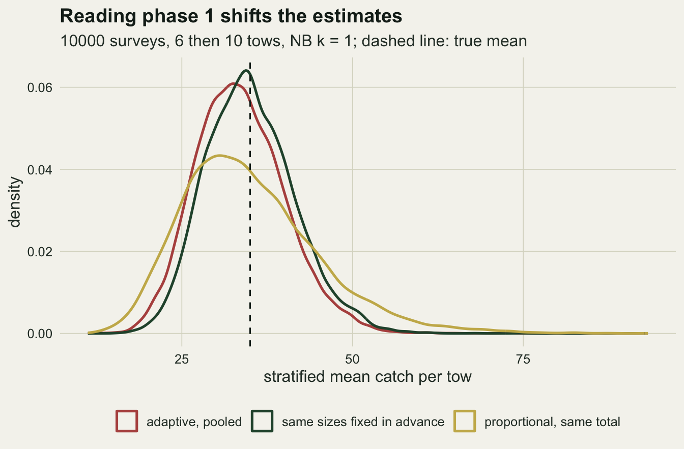
skew <- function(x) mean((x - mean(x))^3) / sd(x)^3
tail_tab <- sapply(list(adaptive = dec$est_ad, fixed = dec$est_fx,
                        proportional = dec$est_pr), function(x)
  c(mean = mean(x), median = median(x), skew = skew(x),
    over_150pc = mean(x > 1.5 * truth), under_75pc = mean(x < 0.75 * truth)))
round(tail_tab, 3)
adaptive fixed proportional
mean 33.576 35.017 34.961
median 33.177 34.608 33.623
skew 0.402 0.404 0.870
over_150pc 0.005 0.007 0.056
under_75pc 0.123 0.074 0.187miss_side <- rbind(
adaptive = c(interval_below = mean(dec$est_ad + 1.96 * dec$se_ad < truth),
interval_above = mean(dec$est_ad - 1.96 * dec$se_ad > truth)),
fixed = c(interval_below = mean(dec$est_fx + 1.96 * dec$se_fx < truth),
interval_above = mean(dec$est_fx - 1.96 * dec$se_fx > truth)))
round(miss_side, 3) interval_below interval_above
adaptive 0.133 0.010
fixed 0.073 0.011Francis reported that his two-phase design reduces the skew of the estimate and the chance of a gross overestimate, and against proportional allocation it does: the skewness of the 10000 estimates is 0.40 against 0.87, and the share of surveys that report more than one and a half times the true mean falls from 0.056 to 0.005. The fixed yardstick gets the same skewness, 0.40, and 0.007 gross overestimates. The shape comes from putting the tows where the fish are, which a fixed allocation does equally well. Reading phase 1 adds the shift. The share of surveys that report less than three quarters of the true mean is 0.123 for the adaptive arm and 0.074 for the fixed one, and the median estimate is 33.2 against 34.6 fish per tow.
The interval failures are one-sided in both arms. The fixed arm’s interval lies wholly below the true mean in 0.073 of surveys and wholly above it in 0.011: with skewed catches a low estimate comes with a low sample variance, so it is also reported as precise. Adaptive allocation adds to that side, 0.133 below against 0.010 above. The coverage it loses is lost on that side: too few fish, reported with too much confidence.
Where the low mean comes from
Write the pooled mean of stratum h, with n1 phase-1 tows and a final total of n_h, as a weighted average of the two phases:
\[\bar y_h = \frac{n_1}{n_h}\,\bar y_{1h} + \frac{n_h - n_1}{n_h}\,\bar y_{2h}.\]
Given phase 1, n_h is settled and the phase-2 tows are fresh draws from the stratum, so the phase-2 mean is conditionally unbiased and its term contributes E(1 - n1/n_h) times the true stratum mean. The phase-1 mean is unbiased on its own, and what is left of the error is a covariance:
\[E(\bar y_h) - \mu_h = \operatorname{Cov}\!\left(\frac{n_1}{n_h},\ \bar y_{1h}\right), \qquad \text{bias of the stratified mean} = \sum_h W_h \operatorname{Cov}\!\left(\frac{n_1}{n_h},\ \bar y_{1h}\right).\]
This is algebra, not a result of the simulation, and it holds for any allocation rule that reads only phase 1. What it does not give is the size: n_h here is the outcome of a greedy choice over four random variances, and there is no closed form for the covariance. The chunk below checks the identity against the simulated bias in all nine cells.
ident_df <- data.frame(observed = sapply(cells, function(cl) cl$tab["adaptive", "bias"]),
                       mcse     = sapply(cells, function(cl) cl$tab["adaptive", "bias_mcse"]),
                       identity = sapply(cells, function(cl) cl$ident),
                       share    = sapply(cells, function(cl) cl$share),
                       k        = sapply(cells, function(cl) cl$k))
ident_gap <- max(abs(ident_df$observed - ident_df$identity) / ident_df$mcse)
round(ident_df, 4)
observed mcse identity share k
1 -0.1129 0.0024 -0.1142 0.3333 0.6
2 -0.0729 0.0019 -0.0706 0.3333 1.0
3 -0.0381 0.0013 -0.0365 0.3333 2.0
4 -0.0867 0.0028 -0.0851 0.6667 0.6
5 -0.0550 0.0022 -0.0584 0.6667 1.0
6 -0.0301 0.0016 -0.0316 0.6667 2.0
7 -0.0607 0.0023 -0.0627 0.7059 0.6
8 -0.0407 0.0019 -0.0410 0.7059 1.0
9 -0.0221 0.0013 -0.0218 0.7059 2.0cor_top <- sapply(cells, function(cl) c(adaptive = cl$cor_ad, taylor = cl$cor_tl,
last_year = cl$cor_ly))
round(cor_top, 2) [,1] [,2] [,3] [,4] [,5] [,6] [,7] [,8] [,9]
adaptive 0.64 0.59 0.48 0.61 0.58 0.49 0.62 0.58 0.49
taylor 0.72 0.71 0.66 0.69 0.70 0.68 0.71 0.71 0.69
last_year 0.01 0.00 -0.01 -0.01 0.00 0.00 0.00 0.00 -0.01top_dec <- dec$top
below_mu <- top_dec$ybar1 < mu_h[4]
w1_split <- c(below = mean(top_dec$w1[below_mu]), above = mean(top_dec$w1[!below_mu]))
w1_cor <- cor(top_dec$w1, top_dec$ybar1)
round(c(share_below = mean(below_mu), w1_split, w1_cor = w1_cor), 3)share_below below above w1_cor
0.559 0.650 0.475 -0.550 contrib <- t(sapply(cells, function(cl) cl$contrib / sum(cl$contrib)))
colnames(contrib) <- paste0("stratum_", 1:H)
round(contrib, 3) stratum_1 stratum_2 stratum_3 stratum_4
[1,] 0.047 0.227 0.348 0.378
[2,] 0.050 0.244 0.352 0.354
[3,] 0.056 0.266 0.351 0.328
[4,] 0.010 0.151 0.391 0.448
[5,] 0.006 0.147 0.392 0.456
[6,] 0.006 0.154 0.401 0.440
[7,] 0.004 0.137 0.401 0.458
[8,] 0.002 0.130 0.420 0.448
[9,] 0.001 0.137 0.431 0.431all_neg <- all(sapply(cells, function(cl) all(cl$contrib < 0)))
deep_two <- contrib[, 3] + contrib[, 4]
cor_s3 <- sapply(cells, function(cl) cl$cor_ad3)
c(all_negative = all_neg, round(range(deep_two), 3), round(range(cor_s3), 2))all_negative
1.000 0.678 0.868 0.480 0.640 The covariance sum and the observed relative bias agree in every cell, the largest gap being 1.5 Monte Carlo standard errors (panel B of the figure below). Every stratum’s term is negative in every cell. The two deepest strata supply most of the bias between them, 0.678 to 0.868 of it across the nine cells; the top stratum alone supplies 0.328 to 0.458, never a majority, and 0.448 in the k = 1 cell with a phase-1 share of 0.71. The mechanism is the same in the third stratum and the top one, and it is easiest to follow in the top one. There the phase-1 mean and the final number of tows are positively correlated, 0.48 to 0.64 across the nine cells (and almost the same in the third stratum, 0.48 to 0.64): a phase 1 that hits a clump has a large sample variance and pulls in extra tows. The weight on phase 1 is n1 divided by those final tows, so it falls as the phase-1 mean rises (correlation -0.55 in the k = 1 cell with a phase-1 share of 0.71). Because negative binomial catches are skewed, phase 1 comes out below the true top-stratum mean more often than above it, in 0.559 of surveys, and in those surveys its tows carry 0.650 of the stratum mean on average, against 0.475 when it came out high. A low start keeps most of its weight; a high start is diluted with fresh tows that are, on average, lower.
Nothing about this depends on the estimator being design-based. The rule reads only recorded catches, so for likelihood inference it is ignorable, which is the point made in Revisits triggered by sightings in occupancy data for a many-site occupancy model. Fitting a negative binomial to each stratum by maximum likelihood does not help either: with no covariates the maximum likelihood estimate of the mean is the sample mean, so it returns the pooled estimate and its bias. Ignorability says the likelihood is correct; it does not say that its estimate is unbiased at the handful of tows per stratum a trawl survey has.
set.seed(4201)
show_rows <- sample.int(nrow(top_dec), 2500)
brk <- quantile(top_dec$ybar1, seq(0, 1, by = 0.1))
top_dec$bin <- cut(top_dec$ybar1, unique(brk), include.lowest = TRUE)
bin_df <- data.frame(ybar1 = tapply(top_dec$ybar1, top_dec$bin, median),
                     w1    = tapply(top_dec$w1, top_dec$bin, mean))
p_weight <- ggplot(top_dec[show_rows, ], aes(ybar1, w1)) +
  geom_jitter(width = 0, height = 0.008, alpha = 0.25, size = 0.8, colour = te_forest) +
  geom_line(data = bin_df, colour = te_rust, linewidth = 1) +
  geom_point(data = bin_df, colour = te_rust, size = 2.2) +
  geom_vline(xintercept = mu_h[4], linetype = "dashed", colour = te_ink) +
  coord_cartesian(xlim = c(0, quantile(top_dec$ybar1, 0.995))) +
  labs(x = "phase-1 mean catch, top stratum", y = "weight on phase 1 (n1 / final tows)",
       title = "A") +
  theme_datasheet()
p_ident <- ggplot(ident_df, aes(identity, observed, colour = factor(k))) +
  geom_abline(slope = 1, intercept = 0, colour = te_line, linewidth = 0.8) +
  geom_errorbar(aes(ymin = observed - 2 * mcse, ymax = observed + 2 * mcse), width = 0) +
  geom_point(size = 2.4) +
  scale_colour_manual(values = c(te_rust, te_gold, te_forest), name = "NB size k") +
  labs(x = "covariance sum / true mean", y = "observed relative bias", title = "B") +
  theme_datasheet() + theme(legend.position = "bottom")
(p_weight | p_ident) + plot_annotation(theme = theme_datasheet())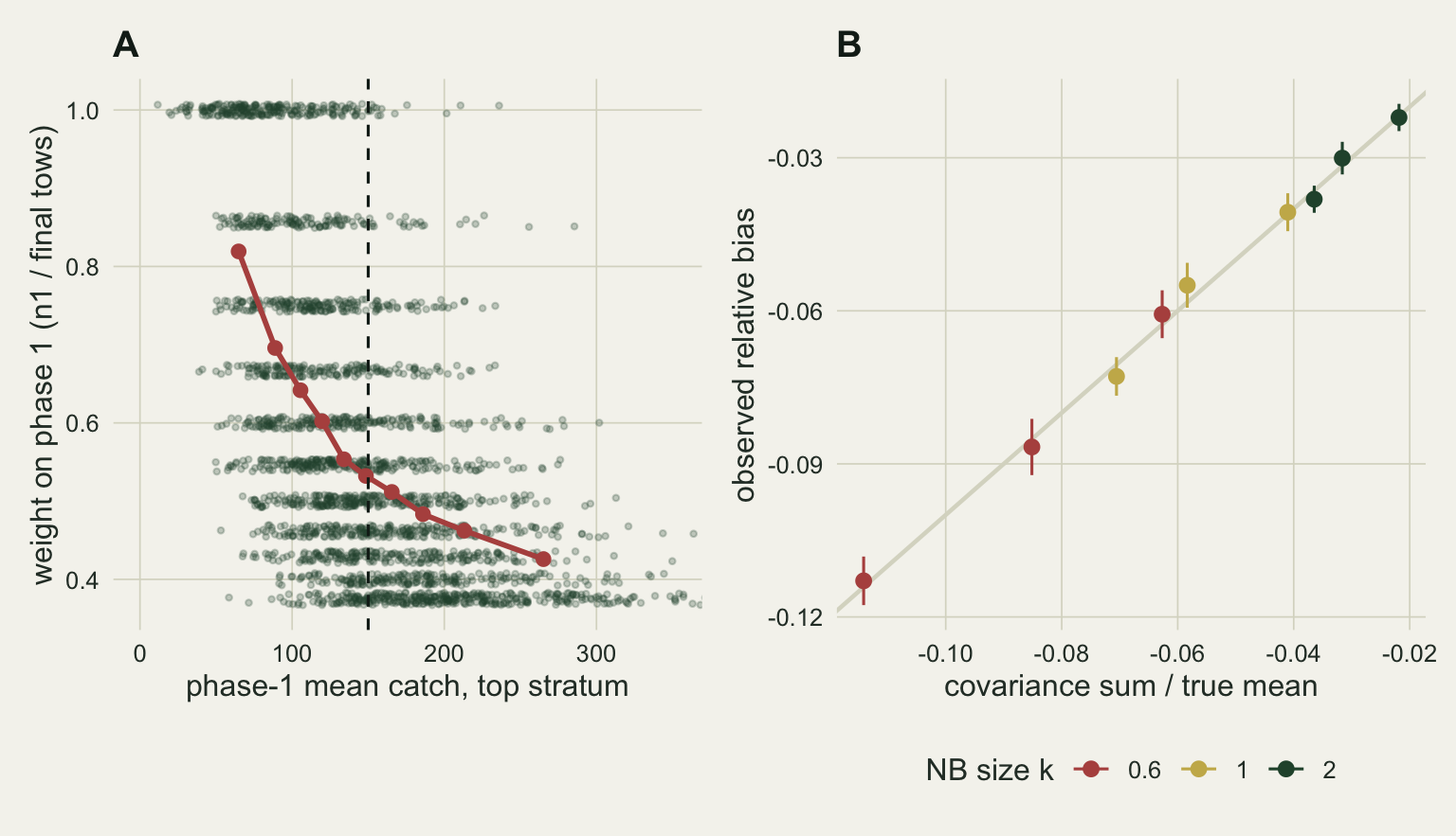
Panel A shows the mechanism in the top stratum for that cell: the weight on phase 1 steps down in discrete levels as extra tows are added, and the binned average falls steadily with the phase-1 mean. Panel B is the identity check.
Phase-1 share and aggregation
ad <- subset(long, arm == "adaptive")
fx <- subset(long, arm == "fixed")
share_df <- data.frame(ad[, c("n1", "m", "k", "share")], bias = ad$bias,
                       cover_ad = ad$cover, cover_fx = fx$cover,
                       loss = fx$cover - ad$cover,
                       rmse_ad = ad$rmse, rmse_fx = fx$rmse,
                       se_ratio_ad = ad$se_ratio, se_ratio_fx = fx$se_ratio,
                       rmse_ratio = ad$rmse / fx$rmse, bias_mse = ad$bias^2 / ad$rmse^2)
round(share_df, 3)
n1 m k share bias cover_ad cover_fx loss rmse_ad rmse_fx se_ratio_ad
1 3 24 0.6 0.333 -0.113 0.740 0.910 0.170 0.263 0.218 0.773
11 3 24 1.0 0.333 -0.073 0.790 0.919 0.129 0.202 0.171 0.799
21 3 24 2.0 0.333 -0.038 0.844 0.930 0.087 0.138 0.120 0.840
31 4 8 0.6 0.667 -0.087 0.779 0.882 0.103 0.289 0.282 0.798
41 4 8 1.0 0.667 -0.055 0.822 0.899 0.077 0.227 0.222 0.826
51 4 8 2.0 0.667 -0.030 0.860 0.919 0.059 0.163 0.157 0.848
61 6 10 0.6 0.706 -0.061 0.828 0.900 0.072 0.242 0.237 0.848
71 6 10 1.0 0.706 -0.041 0.857 0.916 0.059 0.190 0.185 0.866
81 6 10 2.0 0.706 -0.022 0.887 0.929 0.042 0.135 0.130 0.889
se_ratio_fx rmse_ratio bias_mse
1 0.974 1.207 0.184
11 0.963 1.181 0.130
21 0.995 1.153 0.076
31 0.927 1.023 0.090
41 0.943 1.023 0.059
51 0.967 1.038 0.034
61 0.955 1.024 0.063
71 0.966 1.030 0.046
81 0.990 1.045 0.027prac <- subset(share_df, share > 0.5)
lowc <- subset(share_df, share < 0.5)
k2_71 <- subset(share_df, n1 == 6 & k == 2)
ms <- subset(long, arm == "mean_sq")
ms_df <- data.frame(n1 = ms$n1, k = ms$k, share = ms$share, bias = ms$bias,
cover = ms$cover, cover_fx = fx$cover, rmse = ms$rmse,
cor_top = sapply(cells, function(cl) cl$cor_ms))
round(ms_df, 3) n1 k share bias cover cover_fx rmse cor_top
1 3 0.6 0.333 -0.115 0.759 0.910 0.262 0.745
2 3 1.0 0.333 -0.073 0.821 0.919 0.196 0.763
3 3 2.0 0.333 -0.037 0.882 0.930 0.130 0.781
4 4 0.6 0.667 -0.092 0.790 0.882 0.287 0.693
5 4 1.0 0.667 -0.062 0.833 0.899 0.226 0.719
6 4 2.0 0.667 -0.033 0.881 0.919 0.160 0.734
7 6 0.6 0.706 -0.065 0.834 0.900 0.242 0.716
8 6 1.0 0.706 -0.044 0.866 0.916 0.189 0.724
9 6 2.0 0.706 -0.023 0.903 0.929 0.133 0.721ms_prac <- subset(ms_df, share > 0.5)Across the grid the bias shrinks as the phase-1 share grows and as catches become less clumped. In the six cells with two thirds or more of the tows in phase 1, the adaptive mean runs between 2.2 and 8.7 per cent low, and its coverage falls 4.2 to 10.3 points below the fixed yardstick of the same cell. Its root mean square error is 1.02 to 1.05 times the yardstick’s there, so on precision the two tie within a few per cent. Only at the low-share extreme does adaptive allocation clearly lose on precision as well: the ratio is 1.15 to 1.21, the bias 3.8 to 11.3 per cent and the coverage loss 8.7 to 17.0 points.
share_df$k_lab <- factor(sprintf("k = %.1f", share_df$k))
p_bias <- ggplot(share_df, aes(share, bias, colour = k_lab)) +
  geom_hline(yintercept = 0, colour = te_ink, linetype = "dashed") +
  geom_line(linewidth = 0.9) + geom_point(size = 2.2) +
  scale_colour_manual(values = c(te_rust, te_gold, te_forest), name = NULL) +
  labs(x = "phase-1 share of tows", y = "relative bias, adaptive pooled", title = "A") +
  theme_datasheet() + theme(legend.position = "bottom")
p_loss <- ggplot(share_df, aes(share, 100 * loss, colour = k_lab)) +
  geom_hline(yintercept = 0, colour = te_ink, linetype = "dashed") +
  geom_line(linewidth = 0.9) + geom_point(size = 2.2) +
  scale_colour_manual(values = c(te_rust, te_gold, te_forest), name = NULL) +
  labs(x = "phase-1 share of tows", y = "coverage loss against fixed (points)", title = "B") +
  theme_datasheet() + theme(legend.position = "bottom")
(p_bias | p_loss) + plot_layout(guides = "collect") +
  plot_annotation(theme = theme_datasheet() + theme(legend.position = "bottom"))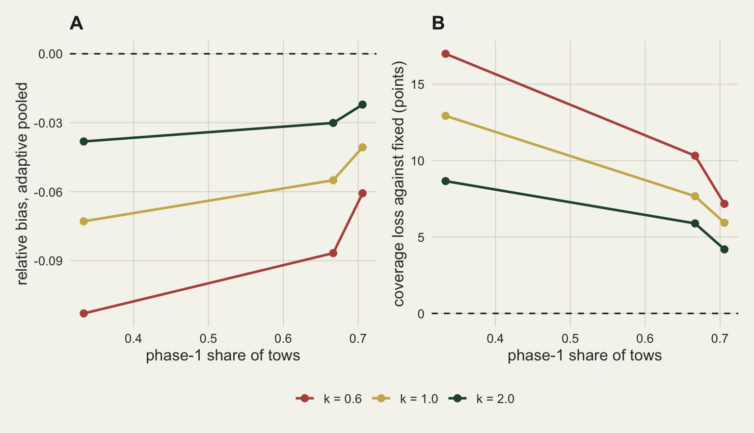
The mildest cell deserves a plain statement. With 0.71 of the tows in phase 1 and k = 2 the bias is 2.2 per cent, and it makes up 0.027 of the mean square error; for a single survey that lean is lost in the noise. The harm there is the interval: 0.887 against 0.929 for the same sizes fixed in advance, because the reported standard error is 0.889 of the true spread against 0.990. The shares on the horizontal axis are not the only thing that changes between the columns, since the two practical splits also differ in n1; the lines join three designs, not a continuous sweep.
The mean-squared form of the rule behaves the same way. It reads the phase-1 mean directly, and the identity applies to it unchanged. In the six practical cells it runs 2.3 to 9.2 per cent low; in the k = 1 cell with a phase-1 share of 0.71 it covers 0.866 against 0.916 for that cell’s fixed yardstick (built from the variance form’s sizes); and the correlation between the phase-1 mean and the final tows in the top stratum is 0.69 to 0.78 across the nine cells, above the variance form’s range.
Four repairs
tl <- subset(long, arm == "taylor")
tl_vs_ad <- data.frame(n1 = ad$n1, k = ad$k, bias_diff = tl$bias - ad$bias,
                       cover_diff = tl$cover - ad$cover, gap_fx = fx$cover - tl$cover)
round(tl_vs_ad, 3)
n1 k bias_diff cover_diff gap_fx
1 3 0.6 0.001 0.019 0.151
2 3 1.0 0.001 0.028 0.102
3 3 2.0 0.002 0.035 0.051
4 4 0.6 -0.005 0.009 0.095
5 4 1.0 -0.006 0.011 0.066
6 4 2.0 -0.003 0.014 0.044
7 6 0.6 -0.004 0.004 0.068
8 6 1.0 -0.003 0.009 0.050
9 6 2.0 -0.002 0.012 0.030ly <- subset(long, arm == "last_year")
ly_gap <- data.frame(n1 = ly$n1, k = ly$k, share = ly$share, bias = ly$bias,
gap = fx$cover - ly$cover, rmse_ratio = ly$rmse / ad$rmse)
round(ly_gap, 3) n1 k share bias gap rmse_ratio
1 3 0.6 0.333 0.002 0.036 1.029
2 3 1.0 0.333 -0.001 0.022 0.999
3 3 2.0 0.333 -0.001 0.015 0.990
4 4 0.6 0.667 0.000 0.012 1.050
5 4 1.0 0.667 0.001 0.007 1.038
6 4 2.0 0.667 0.002 0.010 1.019
7 6 0.6 0.706 0.002 0.006 1.031
8 6 1.0 0.706 0.000 0.006 1.011
9 6 2.0 0.706 0.000 0.004 0.994est_arms <- c("adaptive", "taylor", "last_year", "last_year_moved", "guar_pooled", "guar_phase2",
"mean_sq")
rmse_vs_fx <- sapply(est_arms, function(a) long$rmse[long$arm == a] / fx$rmse)
round(range(rmse_vs_fx), 3)[1] 1.017 1.994l_tab <- low$tab
# moved stock against the adaptive rule: change in MSE against the squared bias removed
mv_cmp <- sapply(list(practical = d_tab, low_share = l_tab), function(tb)
c(mse_rise = tb["last_year_moved", "rmse"]^2 - tb["adaptive", "rmse"]^2,
bias2_removed = tb["adaptive", "bias"]^2 - tb["last_year_moved", "bias"]^2))
round(mv_cmp, 4) practical low_share
mse_rise 0.0069 0.0250
bias2_removed 0.0017 0.0127The first repair to try is to stop each stratum’s allocation from reading its own noisy variance, by fitting Taylor’s power law, log variance against log mean, across the four strata of a survey and allocating from the fitted variances. It fails. The fitted variance of the top stratum is still a function of that stratum’s phase-1 mean, so the allocation still reads the data it will be averaged with; the correlation between the phase-1 mean and the final tows in the top stratum is 0.66 to 0.72, higher than under the raw rule. Its bias stays within 0.006 of the raw Francis bias in every cell and is slightly worse in all six practical cells. Its coverage is 0.4 to 3.5 points better than raw Francis, which still leaves it 3.0 to 15.1 points below the fixed yardstick.
The textbook answer is to keep phase 1 out of the stratum means. Guarantee 2 phase-2 tows per stratum, send the rest by Francis, and estimate each stratum from its phase-2 tows alone: given phase 1 those are ordinary random tows, and the estimate is unbiased, +0.001 in the practical k = 1 cell and -0.002 at the low-share extreme. It throws away 24 of the 34 tows in the practical cell, and its root mean square error nearly doubles, 0.363 against 0.185 for the fixed yardstick; with as few as 2 phase-2 tows in a stratum its interval covers only 0.824. The same allocation with the pooled mean has a bias of only -0.011, but only because just 2 tows are left to adapt; at the low-share extreme, with 16 tows left to adapt, it is back to -0.069. In the 4-then-8 cells all eight phase-2 tows are guaranteed, so that arm is a fixed design there and is not shown.
The repair that works is to feed the Francis rule variances that the estimate will not use. Allocated from an independent survey with n1 tows per stratum, last year’s, the stratified mean is unbiased within Monte Carlo error, +0.000 in the practical cell and +0.002 at the low-share extreme, and covers 0.910 and 0.874 against 0.916 and 0.910 for the yardstick. The correlation between this year’s phase-1 mean and the final tows in the top stratum is -0.01 to 0.01, as it has to be. It does not buy precision: its root mean square error is 0.192 in the practical cell, against 0.190 for the adaptive arm and 0.175 for Neyman on the true standard deviations, and 0.271 against 0.263 at the low-share extreme. No arm that allocates from estimated variances or squared means beat the fixed yardstick on precision in any cell of these runs; the closest came to 1.017 times its root mean square error.
arm_lab <- c(adaptive = "adaptive, pooled", fixed = "fixed in advance (yardstick)",
             neyman = "Neyman on true SDs", proportional = "proportional",
             last_year = "Francis on last year", last_year_moved = "last year, stock moved",
             taylor = "Taylor-smoothed", guar_pooled = "2 guaranteed, pooled",
             guar_phase2 = "2 guaranteed, phase 2 only")
rep_df <- subset(long, arm != "mean_sq" & ((n1 == 6 & k == 1) | (n1 == 3 & k == 0.6)))
rep_df$cell  <- ifelse(rep_df$n1 == 6, "phase-1 share 0.71, k 1", "phase-1 share 0.33, k 0.6")
rep_df$arm_f <- factor(arm_lab[rep_df$arm], levels = rev(arm_lab))
metric_df <- function(col, lab) data.frame(rep_df[, c("cell", "arm_f")], metric = lab,
                                           value = rep_df[[col]])
rep_long <- rbind(metric_df("bias", "relative bias"), metric_df("cover", "coverage"),
                  metric_df("rmse", "relative RMSE"))
rep_long$metric <- factor(rep_long$metric, levels = c("relative bias", "coverage", "relative RMSE"))
ggplot(rep_long, aes(value, arm_f, colour = cell, shape = cell)) +
  geom_point(size = 2.4) +
  facet_wrap(~ metric, scales = "free_x") +
  scale_colour_manual(values = c(te_rust, te_forest), name = NULL) +
  scale_shape_manual(values = c(17, 16), name = NULL) +
  labs(x = NULL, y = NULL, title = "Last year's variances remove the bias without doubling the error") +
  theme_datasheet() + theme(legend.position = "bottom", panel.spacing = unit(1.2, "lines"))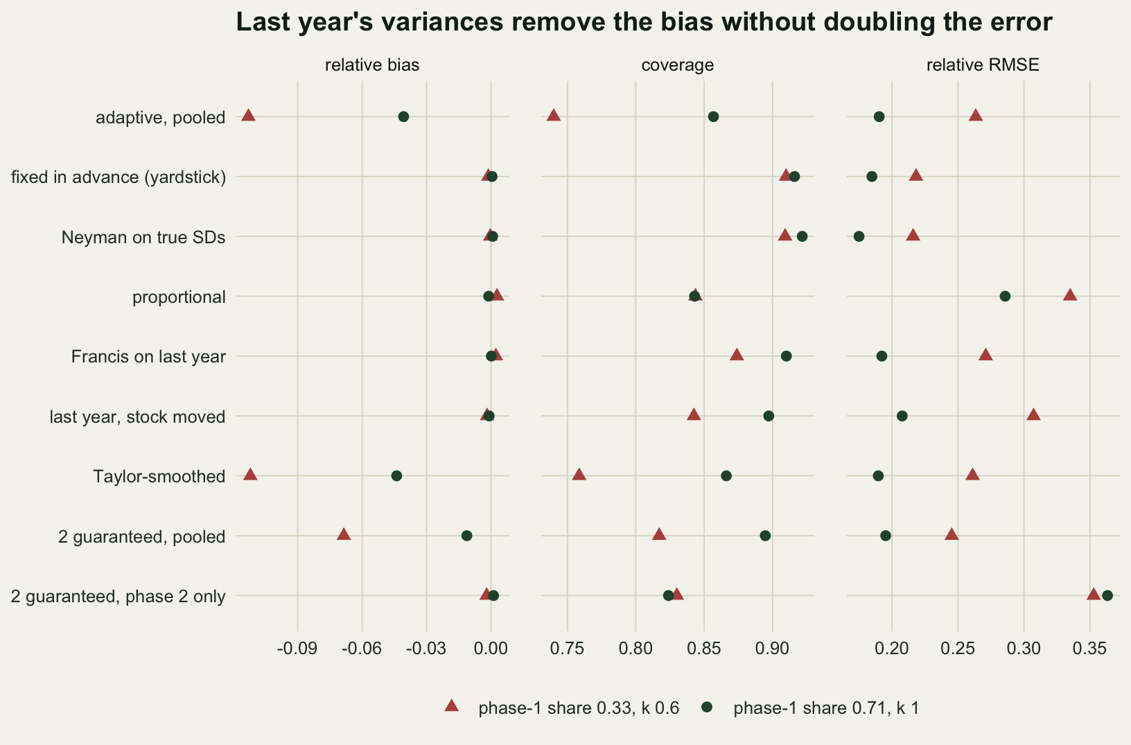
A stock that moves between years is the obvious worry about last year’s variances. When the dense patch sits in the third stratum last year and in the fourth this year, the allocation is aimed at the wrong place, but it is still independent of this year’s catches, so conditional on last year the design is fixed and the stratified mean stays unbiased: -0.001 in the practical cell and -0.002 at the low-share extreme. That part is not a simulation result; it follows from the independence and would hold for any shift. What the shift costs is precision and some coverage, root mean square error 0.208 against 0.192 and coverage 0.897 against 0.910 in the practical cell; the size of that cost belongs to this particular shift. Against the adaptive rule itself, which is what the survey would otherwise run, the moved allocation trades precision for the interval: root mean square error 0.208 against 0.190 and coverage 0.897 against 0.857 in the practical cell, 0.307 against 0.263 and 0.843 against 0.740 at the low-share extreme. In both cells its mean square error, in units of the squared true mean, rises by more than the squared bias it removes: by 0.0069 against 0.0017 in the practical cell and 0.0250 against 0.0127 at the extreme.
What to report
Say how the phase-2 tows were allocated and where the variances that drove the allocation came from: this survey’s phase 1, an earlier survey, or a separate pilot. Give n1 and the final number of tows for every stratum, so a reader can see how much weight each phase carries. If the allocation read phase 1 and both phases were pooled, say that the stratified mean is expected to lean low and its interval to be short; with two thirds or more of the tows in phase 1, the lean in these runs was 2.2 to 8.7 per cent and the interval’s shortfall against a fixed design 4.2 to 10.3 points, larger with more clumped catches and a smaller phase 1.
For the next survey, the cheapest change is to allocate phase 2 from variances the estimate will not reuse. Last year’s survey did that here with no bias, with coverage within 1.2 points of the fixed yardstick in the practical cells (3.6 at the low-share extreme), and at a root mean square error 0.99 to 1.05 times that of the adaptive rule. When the stock has moved since last year, the same allocation still removes the bias and most of the interval’s shortfall, but in the one shift run here at a cost in precision larger than the bias it removes. A Taylor-law smoothing of this year’s phase-1 variances is not a substitute, and neither is a model-based fit of the same catches.
When judging an allocation rule by simulation, compare coverage with a fixed design of the same size, not with 0.95. With a handful of skewed catches per stratum, the fixed design here covered 0.882 to 0.929 on its own.
Honest limits
One population shape was simulated: four strata with fixed weights and means, independent negative binomial catches with the same k in every stratum, and no spatial structure inside a stratum. Real strata have trends in depth and patches that span several tows, and the size of the bias will move with all of this. A low lean is the expected direction for right-skewed catches, from the identity and from the positive link between a stratum’s phase-1 mean and its sample variance: for independent catches the covariance of the sample mean and the sample variance is the third central moment divided by the number of tows, positive for any right-skewed catch distribution. That link does not fix the sign under a greedy rule over several strata in general, and the size can only be simulated.
The fixed yardstick uses the adaptive arm’s average final sizes, which are known only after the simulation. It says what the same allocation would do if it did not read the data; it is not a design a survey could choose in advance, and the practical comparison for last year’s allocation is the adaptive arm itself.
The Francis rule is run here in its plain greedy form, one tow at a time on the sample variances of numbers caught, with the mean-squared form as a check. A survey may add a minimum per stratum, cap the phase-2 tows a stratum can take, or allocate on catch weight; of these only a minimum was run, as the guaranteed-tows arm, and it shrank the bias only by leaving fewer tows to adapt.
The phase-2-only estimator is unbiased and wasteful. The standard way to recover the information it throws away without bringing the bias back is Rao-Blackwellisation, averaging the unbiased estimator over the ways the final sample could have been split into phases consistently with the rule, the device that runs through the adaptive designs in Thompson and Seber (1996). For a greedy rule over four strata that average has no simple form, and it was not implemented, so how much of the lost precision it recovers here is not known from these runs.
Last year’s survey here has only n1 tows per stratum, the size of this year’s phase 1. A full-size survey from last year would give better variances, and a one-shot Neyman allocation on last year’s standard deviations was not run.
The moved stock is one shift, the dense patch trading places between the two deepest strata. Unbiasedness under any shift follows from independence; the cost in precision measured here does not transfer to other shifts. Intervals are the usual normal ones on the stratified mean. A log-scale or bootstrap interval might cover better for every arm, and was not tried. Nor was a bootstrap bias correction of the adaptive estimate, which in Manly’s (2004) study removed about half of the bias.
References
Francis RICC 1984 New Zealand Journal of Marine and Freshwater Research 18(1):59-71 (10.1080/00288330.1984.9516030)
Jolly GM, Hampton I 1990 Canadian Journal of Fisheries and Aquatic Sciences 47(7):1282-1291 (10.1139/f90-147)
Manly BFJ 2004 Environmental and Ecological Statistics 11(4):367-383 (10.1007/s10651-004-4184-y)
Moradi M, Salehi M 2010 Journal of Statistical Planning and Inference 140(4):1030-1037 (10.1016/j.jspi.2009.10.003)
Whitehead J 1986 Biometrika 73(3):573-581 (10.1093/biomet/73.3.573)
Cochran WG 1977 Sampling Techniques, 3rd edn, Wiley (ISBN 978-0-471-16240-7)
Thompson SK, Seber GAF 1996 Adaptive Sampling, Wiley (ISBN 978-0-471-55871-2)