library(ggplot2)

te_pal <- list(forest = "#275139", green = "#2f8f63", sage = "#93a87f",
               clay = "#b5534e", gold = "#cda23f", line = "#dad9ca",
               ink = "#16241d", paper = "#f5f4ee")

theme_te <- function() {
  theme_minimal(base_size = 12) +
    theme(panel.grid.minor = element_blank(),
          panel.grid.major = element_line(colour = "#e7e6dc"),
          plot.background = element_rect(fill = "#f5f4ee", colour = NA),
          panel.background = element_rect(fill = "#f5f4ee", colour = NA),
          plot.title = element_text(face = "bold", colour = te_pal$ink),
          axis.title = element_text(colour = "#2c3a31"))
}List-length analysis for opportunistic data
R
citizen science
monitoring
ecology tutorial
ggplot2
Opportunistic species records carry the observer as well as the species. This R tutorial conditions a trend on list length and measures what is left over.
A county recorder hands you twenty years of casual records for a scarce plant: date, grid square, recorder, nothing else. No survey design, no fixed sites, no repeat visits by protocol. The number of records per year has tripled. Somebody wants to know whether the plant is spreading, and the honest first answer is that the record count cannot tell you, because the same tripling would appear if the plant had stayed exactly where it was and the recording group had simply grown.
The usual next move is to divide by something. Divide the target species records by the total records for that year, and you have a reporting rate that looks effort-free. This tutorial measures what that division actually does. It simulates a record stream in which the truth is known by construction, computes the two obvious naive trends and the list-length correction on the same data, and reports how far each lands from the truth. The two naive summaries here disagree with each other by more than a factor of four, and the truth sits between them.
That effort and detection can masquerade as ecology is not news on this blog. First flowering date and sampling effort showed it for a date-of-first-record statistic, and sampling bias in presence-only models showed the same confound acting in space rather than in time. What is new here is the method rather than the finding: a temporal trend estimated from records that were never designed to support one, using the length of the observer’s own list as the effort covariate. The records are assumed to have been through the tidying in cleaning GBIF occurrence data already; this post starts where that one stops.
A record stream where the truth is known
The simulated recording area has 1200 sites and a background community of 60 species whose occupancy never changes. Sites differ in quality on one axis, and better sites hold more of the background species and are also better for the target species, which is the coupling that later turns out to matter most.
A visit produces one list. The observer arrives at a site with a latent effort value, meaning everything that makes a visit productive rolled into one number: time spent, patience, skill, weather. Every species present at the site is written down with a probability that rises with that effort, so the list is the set of species found. The target species is one more species on the same list, with its own detectability.
Two things change over the twenty years. Visits per year rise from 260 to 580, which is a pure sample-size change and biases nothing. Latent effort per visit drifts upward at 0.11 on the log-odds scale each year, which raises the detection probability of every species including the target, and that one does bias things. Against that, the target species genuinely spreads: its site-level occupancy rises by 0.06 log-odds per year, which is the number every estimator below is trying to recover.
n_years  <- 20
n_sites  <- 1200
n_other  <- 60
b_true   <- 0.06
t0_logit <- -0.85
sq_other <- 0.35
sq_targ  <- 0.25
a_target <- 0.55
eff_sd   <- 0.65
eff_drift <- 0.11
nv_year  <- round(seq(260, 580, length.out = n_years))
yr       <- seq_len(n_years) - (n_years + 1) / 2

set.seed(20260802)
q_site  <- rnorm(n_sites)
g_other <- rnorm(n_other, -0.35, 1.05)
a_other <- rnorm(n_other, -0.90, 1.10)
occ_other <- matrix(runif(n_sites * n_other), n_sites, n_other) <
  plogis(outer(sq_other * q_site, g_other, "+"))

round(c(years = n_years, sites = n_sites, background_species = n_other,
        visits_total = sum(nv_year), visits_first_year = nv_year[1],
        visits_last_year = nv_year[n_years],
        true_occupancy_slope = b_true, effort_drift_per_year = eff_drift,
        effort_sd = eff_sd, target_detection_intercept = a_target,
        mean_species_per_site = mean(rowSums(occ_other))), 4)
years sites
20.0000 1200.0000
background_species visits_total
60.0000 8400.0000
visits_first_year visits_last_year
260.0000 580.0000
true_occupancy_slope effort_drift_per_year
0.0600 0.1100
effort_sd target_detection_intercept
0.6500 0.5500
mean_species_per_site
26.2575 The one number that needs care is the truth itself. The occupancy trend is set at the site level, and sites differ, so the trend in occupancy averaged over sites is slightly flatter on the log-odds scale than the site-level slope. Every comparison below uses the averaged version, because that is what a trend for the region means.
mean_psi <- function(u, sqt = sq_targ, b_year = b_true)
  mean(plogis(t0_logit + b_year * u + sqt * q_site))
true_slope <- function(sqt = sq_targ, b_year = b_true)
  unname(coef(lm(qlogis(sapply(yr, mean_psi, sqt, b_year)) ~ yr))[2])

b_marg <- true_slope()
round(c(site_level_slope = b_true, regional_slope = b_marg,
        occupancy_year_1 = mean_psi(yr[1]),
        occupancy_year_20 = mean_psi(yr[n_years])), 4)
site_level_slope regional_slope occupancy_year_1 occupancy_year_20
0.0600 0.0592 0.1970 0.4306 The regional trend is 0.0592 log-odds per year against a site-level 0.06, and mean occupancy runs from 0.197 to 0.4306 over the twenty years. From here on, 0.0592 is the truth.
The simulator returns one row per list: the year, the list length, the list length excluding the target, whether the target was on it, and the latent effort, which no analyst would ever see but which is useful as a reference. Lists on which nothing at all was found are dropped, because a recorder who finds nothing submits nothing, and that omission is part of the data-generating process rather than a modelling convenience.
sim_stream <- function(b_year = b_true, eff_slope = eff_drift, skill_slope = 0,
                       site_slope = 0, a_t = a_target, sqt = sq_targ,
                       nv = nv_year) {
  ntot <- sum(nv); last <- cumsum(nv); first <- last - nv + 1L
  eff <- numeric(ntot); n_bg <- integer(ntot); tg <- integer(ntot)
  for (i in seq_len(n_years)) {
    k <- first[i]:last[i]
    nvi <- nv[i]
    sid <- sample.int(n_sites, nvi, replace = TRUE,
                      prob = exp(site_slope * yr[i] * q_site))
    ee <- rnorm(nvi, eff_slope * yr[i], eff_sd)
    occ_t <- runif(n_sites) < plogis(t0_logit + b_year * yr[i] + sqt * q_site)
    tg[k] <- as.integer(occ_t[sid] &
                          runif(nvi) < plogis(a_t + ee + skill_slope * yr[i]))
    pp <- plogis(outer(ee, a_other, "+")) * occ_other[sid, , drop = FALSE]
    n_bg[k] <- rowSums(matrix(runif(nvi * n_other), nvi, n_other) < pp)
    eff[k] <- ee
  }
  keep <- (n_bg + tg) > 0
  data.frame(year = rep(yr, nv)[keep], listlen = (n_bg + tg)[keep],
             bg = n_bg[keep], target = tg[keep], effort = eff[keep])
}

set.seed(20260802)
d <- sim_stream()
early <- d$year < -4.5
late  <- d$year > 4.5
round(c(lists = nrow(d), records = sum(d$listlen),
        mean_list_length_first_5_years = mean(d$listlen[early]),
        mean_list_length_last_5_years = mean(d$listlen[late]),
        target_records = sum(d$target),
        correlation_log_list_with_effort = cor(log(d$listlen), d$effort)), 4)
lists records
8337.0000 76162.0000
mean_list_length_first_5_years mean_list_length_last_5_years
5.1236 12.3079
target_records correlation_log_list_with_effort
1836.0000 0.7823 The stream holds 8337 lists carrying 76162 records, of which 1836 are the target species. Mean list length runs from 5.1236 species in the first five years to 12.3079 in the last five, so effort per visit has more than doubled over a period in which occupancy also roughly doubled, from 0.197 to 0.4306. Log list length correlates with the latent effort at 0.7823, which is high enough for the proxy to be useful and low enough to matter later.
Three trends from one stream
Two naive estimators are in common use and they are not the same estimator. The first divides target records by all records for that year, which is what people mean by a reporting rate when they have records rather than lists. The second treats each list as a trial and asks what fraction of lists contain the target, which is the reporting rate of the list-length literature. The correction adds one term to the second: the logarithm of the list length, as a covariate for how much effort the visit represents.
naive_records <- function(dd) {
  ag <- aggregate(cbind(hit = target, all = listlen) ~ year, dd, sum)
  glm(cbind(hit, all - hit) ~ year, binomial, ag)
}
naive_lists <- function(dd) glm(target ~ year, binomial, dd)
lla_log     <- function(dd) glm(target ~ year + log(listlen), binomial, dd)

m_rec <- naive_records(d); m_lst <- naive_lists(d); m_lla <- lla_log(d)
print(round(summary(m_rec)$coefficients, 4))
Estimate Std. Error z value Pr(>|z|)
(Intercept) -3.7693 0.0291 -129.5572 0
year 0.0206 0.0048 4.3321 0print(round(summary(m_lst)$coefficients, 4)) Estimate Std. Error z value Pr(>|z|)
(Intercept) -1.4839 0.0315 -47.1476 0
year 0.0983 0.0053 18.5351 0print(round(summary(m_lla)$coefficients, 4)) Estimate Std. Error z value Pr(>|z|)
(Intercept) -3.4344 0.1319 -26.0356 0
year 0.0443 0.0062 7.1558 0
log(listlen) 0.9583 0.0604 15.8778 0round(c(truth = b_marg, records = coef(m_rec)[2], lists = coef(m_lst)[2],
list_length = coef(m_lla)[2],
ratio_of_naive_slopes = coef(m_lst)[2] / coef(m_rec)[2]), 4) truth records.year
0.0592 0.0206
lists.year list_length.year
0.0983 0.0443
ratio_of_naive_slopes.year
4.7678 One dataset, three answers. The record share gives 0.0206 log-odds per year, the list rate gives 0.0983, and the list-length model gives 0.0443 against a truth of 0.0592. The two naive numbers differ from each other by a factor of 4.7678, and an analyst who had only one of them would report either a plant creeping up or a plant expanding fast. Both naive models fit well by any usual standard, with the year term at a z value of 4.3321 in one and 18.5351 in the other.
A single dataset is an anecdote, so the same three estimators are run over 30 independent streams, along with the alternative specifications used later and one reference estimator that no analyst can compute: the same logistic regression with the latent effort itself in place of list length. The whole set is also run on streams with the effort drift switched off, which gives the target that a list-level model can reach at best.
lcat  <- function(x) cut(x, c(0, 1, 3, 8, Inf), labels = c("1", "2-3", "4-8", "9+"))
all_slopes <- function(dd) {
  bench <- function(mn) unname(coef(glm(target ~ year, binomial,
                                        dd[dd$listlen >= mn, ]))[2])
  c(records = unname(coef(naive_records(dd))[2]),
    lists   = unname(coef(naive_lists(dd))[2]),
    log_len = unname(coef(lla_log(dd))[2]),
    raw_len = unname(coef(glm(target ~ year + listlen, binomial, dd))[2]),
    binned  = unname(coef(glm(target ~ year + lcat(listlen), binomial, dd))[2]),
    bench4  = bench(4), bench10 = bench(10),
    exclude = unname(coef(glm(target ~ year + log1p(bg), binomial, dd))[2]),
    effort  = unname(coef(glm(target ~ year + effort, binomial, dd))[2]),
    kept4   = mean(dd$listlen >= 4), kept10 = mean(dd$listlen >= 10))
}

set.seed(20260802)
n_rep <- 30
drift_rep <- t(replicate(n_rep, all_slopes(sim_stream())))
flat_rep  <- t(replicate(n_rep, all_slopes(sim_stream(eff_slope = 0))))
c(replicates = n_rep)
replicates
30 print(round(rbind(drift_mean = colMeans(drift_rep),
drift_sd = apply(drift_rep, 2, sd),
no_drift_mean = colMeans(flat_rep)), 4)) records lists log_len raw_len binned bench4 bench10 exclude
drift_mean 0.0155 0.0921 0.0354 0.0426 0.0505 0.0766 0.0501 0.0660
drift_sd 0.0047 0.0063 0.0072 0.0076 0.0066 0.0068 0.0103 0.0074
no_drift_mean 0.0402 0.0503 0.0511 0.0512 0.0509 0.0510 0.0516 0.0507
effort kept4 kept10
drift_mean 0.0538 0.8768 0.4253
drift_sd 0.0090 0.0030 0.0046
no_drift_mean 0.0508 0.8925 0.3406round(c(truth = b_marg,
bias_records = mean(drift_rep[, "records"]) - b_marg,
bias_lists = mean(drift_rep[, "lists"]) - b_marg,
bias_log_len = mean(drift_rep[, "log_len"]) - b_marg,
percent_lost_by_record_share =
100 * (1 - mean(drift_rep[, "records"]) / b_marg),
percent_added_by_list_rate =
100 * (mean(drift_rep[, "lists"]) / b_marg - 1),
percent_lost_by_list_length =
100 * (1 - mean(drift_rep[, "log_len"]) / b_marg)), 4) truth bias_records
0.0592 -0.0438
bias_lists bias_log_len
0.0328 -0.0238
percent_lost_by_record_share percent_added_by_list_rate
73.8775 55.3975
percent_lost_by_list_length
40.1652 Over 30 streams the record share averages 0.0155, the list rate 0.0921 and the list-length model 0.0354, against the truth of 0.0592. As percentages of the truth, the record share loses 73.9 per cent of the trend, the list rate adds 55.4 per cent, and the list-length model loses 40.2 per cent. The correction moves the estimate a long way in the right direction and then past the truth, turning the list rate’s overshoot into a shortfall.
Two features of that table deserve attention before the shortfall is diagnosed. The first is that the two naive estimators are biased in opposite directions, which means the popular defence that a reporting rate is conservative is not available: it depends entirely on which denominator was used. The second is that the reference estimator, the one that gets to see the latent effort itself, averages 0.0538 rather than 0.0592. Even perfect knowledge of effort does not return the occupancy trend, and the next section but one explains why.
yrs   <- sort(unique(d$year))
rec_y <- tapply(d$target, d$year, sum) / tapply(d$listlen, d$year, sum)
lst_y <- tapply(d$target, d$year, mean)
psi_y <- sapply(yrs, mean_psi)
adj_m <- glm(target ~ factor(year) + log(listlen), binomial, d)
adj_y <- c(0, coef(adj_m)[2:n_years])

ctr <- function(v) v - mean(v)
ser_lab <- c("Target share of all records", "Fraction of lists with the target",
             "Adjusted for list length", "True occupancy")
ser <- data.frame(
  year = rep(yrs, 4),
  val = c(ctr(qlogis(rec_y)), ctr(qlogis(lst_y)), ctr(adj_y), ctr(qlogis(psi_y))),
  series = factor(rep(ser_lab, each = n_years), levels = ser_lab))
sl <- data.frame(series = factor(ser_lab, levels = ser_lab),
                 slope = c(coef(m_rec)[2], coef(m_lst)[2], coef(m_lla)[2], b_marg))
sl$x <- min(yrs); sl$xend <- max(yrs)
sl$y <- sl$slope * sl$x; sl$yend <- sl$slope * sl$xend
ser_col <- c("#b5534e", "#cda23f", "#2f8f63", "#16241d")
names(ser_col) <- ser_lab

ggplot(ser, aes(year, val, colour = series)) +
  geom_hline(yintercept = 0, colour = te_pal$line, linewidth = 0.8) +
  geom_point(size = 1.9, alpha = 0.85) +
  geom_segment(data = sl, aes(x = x, xend = xend, y = y, yend = yend,
                              colour = series), inherit.aes = FALSE,
               linewidth = 0.9) +
  scale_colour_manual(values = ser_col, name = NULL) +
  scale_x_continuous(breaks = seq(-9.5, 9.5, by = 5),
                     labels = c("year 1", "year 6", "year 11", "year 16")) +
  labs(x = "year of the recording period",
       y = "log-odds, centred on the study mean",
       title = "Two naive trends bracket the truth and neither one is it") +
  theme_te() +
  theme(legend.position = "right")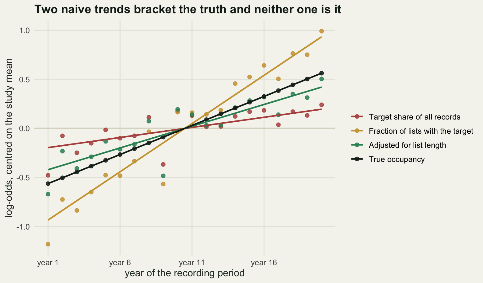
Why the two naive rates disagree
The two naive estimators cannot both be right, and the reason they differ is worth working out, because it decides the direction of the error in a real dataset.
The fraction of lists carrying the target is the probability that the species is present at the visited site and detected on that visit. Rising effort raises the detection half, so the fraction climbs faster than occupancy does. That bias is upward whenever effort rises, and its size depends on how far the target’s detection probability is from one.
The share of all records is a different quantity: the numerator is the same, but the denominator is the total number of records, which is the summed length of every list. Rising effort inflates the denominator too, and it inflates it faster than the numerator whenever the target is already easier to detect than the average species on the list, because the target’s own detection probability is nearer to its ceiling. The share can therefore fall while the species spreads. To see the whole range, the target’s detectability is swept from well below the background average to well above it, holding everything else fixed.
det_grid <- c(-1, 0, 0.55, 1.5, 2.5, 3.5)
set.seed(20260802)
det_sweep <- t(sapply(det_grid, function(a) {
  r <- t(sapply(1:10, function(i) {
    dd <- sim_stream(a_t = a)
    c(unname(coef(naive_records(dd))[2]), unname(coef(naive_lists(dd))[2]),
      unname(coef(glm(target ~ year + lcat(listlen), binomial, dd))[2]),
      mean(dd$target))
  }))
  c(detection_intercept = a, record_share = mean(r[, 1]), list_rate = mean(r[, 2]),
    binned_list_length = mean(r[, 3]), fraction_of_lists = mean(r[, 4]))
}))
print(round(det_sweep, 4))
detection_intercept record_share list_rate binned_list_length
[1,] -1.00 0.0504 0.1196 0.0719
[2,] 0.00 0.0284 0.1037 0.0584
[3,] 0.55 0.0157 0.0924 0.0506
[4,] 1.50 0.0019 0.0810 0.0457
[5,] 2.50 -0.0116 0.0648 0.0307
[6,] 3.50 -0.0157 0.0610 0.0315
fraction_of_lists
[1,] 0.1124
[2,] 0.1822
[3,] 0.2189
[4,] 0.2665
[5,] 0.2988
[6,] 0.3154c(replicates_per_level = 10)replicates_per_level
10 round(c(truth = b_marg), 4) truth
0.0592 The record share slope falls with detectability, from 0.0504 for a target harder to find than the background average down to -0.0157 for a conspicuous one. It passes through zero just above a detection intercept of 1.5, where the target already appears on 0.2665 of lists: at that point the species is spreading at 0.0592 log-odds per year and its share of the records is flat, at 0.0019. Beyond that the share declines while the species increases. The mechanism sits entirely in the denominator, and no amount of care with the numerator fixes it.
The list rate slope falls too, from 0.1196 to 0.061, for the opposite reason: a species already found whenever it is present has little detection left to gain from extra effort, so there is less upward bias to have. For the most conspicuous target in the sweep the list rate is the least biased of the three estimators.
The awkward column is the corrected one, which also falls, from 0.0719 to 0.0315. For a conspicuous species the correction makes matters worse rather than better. That is not a coding error and it is the first sign of the mechanism that closes this post: when the target’s detection has nothing left to gain from effort, conditioning on list length removes no bias and introduces one, because list length carries site quality as well as effort. The last section measures that directly.
What conditioning on list length actually buys
The reference estimator that sees the latent effort returned 0.0538 rather than the true 0.0592, and with the drift switched off it returned 0.0508. A list-level model is not estimating an occupancy trend at all: it is estimating the trend in the probability that a visit yields a record, which is occupancy multiplied by detection. Differentiating the log-odds of that product gives a predictable attenuation, by a factor of one minus occupancy over one minus the product.
gauss_mean <- function(f, mu, sdv) {
  x <- seq(-6, 6, length.out = 4001)
  sum(dnorm(x) * f(mu + sdv * x)) * (x[2] - x[1])
}
psi_bar <- mean(sapply(yr, mean_psi))
p_bar   <- gauss_mean(plogis, a_target, eff_sd)
pred_factor <- (1 - psi_bar) / (1 - psi_bar * p_bar)
b_fix <- pred_factor * b_marg
b_flat <- mean(flat_rep[, "effort"])
round(c(mean_occupancy = psi_bar, mean_detection = p_bar,
        predicted_attenuation = pred_factor,
        reachable_slope = b_fix,
        measured_no_drift_slope = b_flat,
        measured_attenuation = b_flat / b_marg,
        record_share_no_drift = mean(flat_rep[, "records"]),
        record_share_attenuation = mean(flat_rep[, "records"]) / b_marg,
        one_minus_occupancy = 1 - psi_bar), 4)
mean_occupancy mean_detection predicted_attenuation
0.3059 0.6230 0.8575
reachable_slope measured_no_drift_slope measured_attenuation
0.0508 0.0508 0.8582
record_share_no_drift record_share_attenuation one_minus_occupancy
0.0402 0.6785 0.6941 Mean occupancy over the study is 0.3059 and the target’s mean detection probability is 0.623, which predicts an attenuation factor of 0.8575 and a reachable slope of 0.0508. The measured value with the drift switched off is also 0.0508, an attenuation of 0.8582. Prediction and measurement agree closely, so the gap between a reporting trend and an occupancy trend is structural rather than accidental. It closes only as detection approaches one, and it is the reason the next post in this cluster builds detection histories instead. Note also that the same reference estimator under drift gave 0.0538 rather than 0.0508: even a perfect effort covariate leaves a little, because the product of occupancy and detection is not exactly linear on the log-odds scale in either of them.
The record share is attenuated harder, to 0.0402 with no drift at all, a factor of 0.6785. That one also has a closed form: the share is a small proportion of a very large denominator, so its log-odds is effectively its logarithm, and a trend in the logarithm of occupancy is the trend in the log-odds multiplied by one minus occupancy, which is 0.6941 here. Two of the three estimators are therefore biased before any effort drift exists at all.
What the list length is doing can be seen directly. Split the stream into its first and last five years and plot the chance that the target appears against how many species were on the list.
per <- ifelse(early, "first 5 years", ifelse(late, "last 5 years", NA))
dd2 <- d[!is.na(per), ]
dd2$period <- factor(per[!is.na(per)], levels = c("first 5 years", "last 5 years"))
log_ref <- mean(log(dd2$listlen))
dd2$cl <- log(dd2$listlen) - log_ref
m_shape <- glm(target ~ cl * period, binomial, dd2)
print(round(summary(m_shape)$coefficients, 4))
Estimate Std. Error z value Pr(>|z|)
(Intercept) -1.7256 0.1069 -16.1440 0.0000
cl 1.0660 0.1697 6.2822 0.0000
periodlast 5 years 0.6012 0.1225 4.9094 0.0000
cl:periodlast 5 years -0.0818 0.1992 -0.4104 0.6815brk <- c(0, 1, 2, 3, 5, 8, 12, 20, Inf)
dd2$bin <- cut(dd2$listlen, brk)
emp <- aggregate(cbind(target, listlen) ~ bin + period, dd2, mean)
emp$n <- aggregate(target ~ bin + period, dd2, length)$target
emp <- emp[emp$n >= 25, ]
grd <- expand.grid(listlen = exp(seq(log(1), log(max(dd2$listlen)),
length.out = 120)),
period = levels(dd2$period))
grd$cl <- log(grd$listlen) - log_ref
grd$fit <- predict(m_shape, grd, type = "response")
round(c(reference_list_length = exp(log_ref),
lists_in_first_5_years = sum(dd2$period == "first 5 years"),
lists_in_last_5_years = sum(dd2$period == "last 5 years"),
smallest_bin_kept = min(emp$n),
period_midpoint_gap_years = 15,
gap_implied_by_reachable_slope = 15 * b_fix), 4) reference_list_length lists_in_first_5_years
8.0437 1424.0000
lists_in_last_5_years smallest_bin_kept
2731.0000 27.0000
period_midpoint_gap_years gap_implied_by_reachable_slope
15.0000 0.7620 ggplot(grd, aes(listlen, fit, colour = period)) +
geom_line(linewidth = 1) +
geom_point(data = emp, aes(listlen, target, colour = period, size = n)) +
scale_colour_manual(values = c(te_pal$gold, te_pal$forest), name = NULL) +
scale_size_continuous(range = c(1.8, 5), name = "lists in bin") +
scale_x_log10(breaks = c(1, 2, 5, 10, 20, 40)) +
labs(x = "species on the list", y = "probability the target is on the list",
title = "At a given list length the target turns up more often late on") +
theme_te() +
theme(legend.position = "right")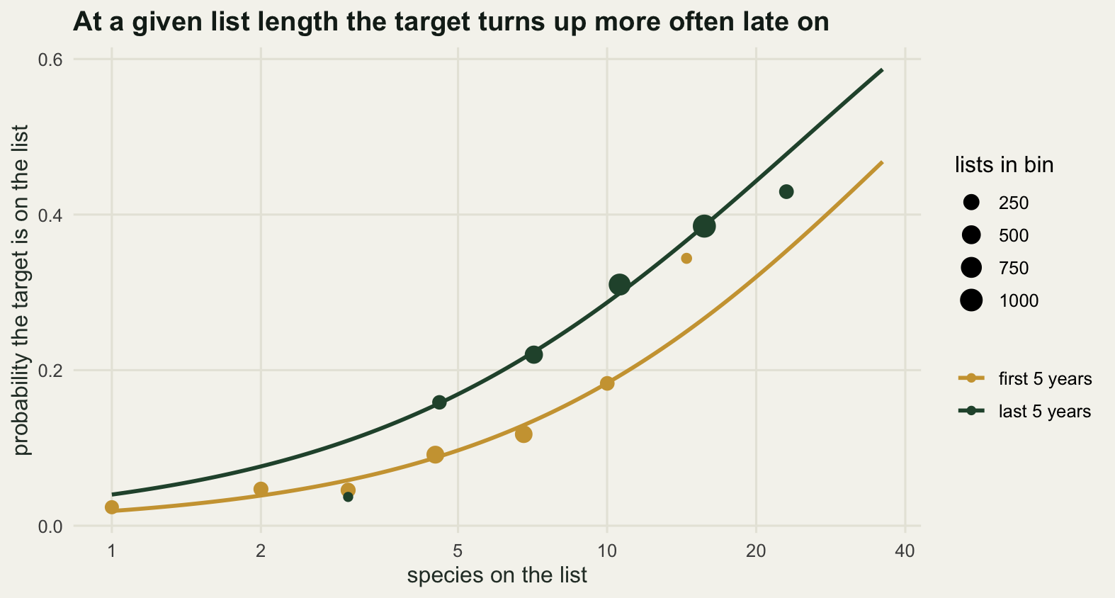
The two curves are the argument for the method in one picture. At the reference list of 8.0437 species the late period sits 0.6012 log-odds above the early period, with a standard error of 0.1225, and that gap is not effort, because the comparison holds list length fixed. Fifteen years separate the midpoints of the two periods, so the reachable slope of 0.0508 predicts a gap of 0.762, which is more than the 0.6012 observed on this stream.
The interaction is the part worth checking rather than assuming. The slope on log list length changes by -0.0818 between the periods, with a p-value of 0.6815, so a single common effort response is adequate here. That is a property of this simulator, in which effort acts the same way on every species in every year, and it is one of the first things to test on real data, where a change in what recorders write down can change the shape of the response and not just its position.
Four ways to put list length in the model
Nothing so far has justified the logarithm. Four specifications are in circulation: the logarithm of the list length, the raw count, a small set of length classes, and a benchmark rule that throws away short lists and then fits the naive list model to what remains. All four were computed on the same 30 streams, together with a fifth that keeps the logarithm but removes the target species from its own list length.
form_lab <- c(lists = "no effort term", log_len = "log(list length)",
              raw_len = "raw list length", binned = "length classes",
              bench4 = "lists of 4 or more", bench10 = "lists of 10 or more",
              exclude = "log length, target removed", effort = "latent effort (oracle)")
form_tab <- rbind(estimate = colMeans(drift_rep[, names(form_lab)]),
                  sd = apply(drift_rep[, names(form_lab)], 2, sd),
                  bias_vs_truth = colMeans(drift_rep[, names(form_lab)]) - b_marg,
                  bias_vs_reachable = colMeans(drift_rep[, names(form_lab)]) - b_fix)
colnames(form_tab) <- form_lab
print(round(t(form_tab), 4))
estimate sd bias_vs_truth bias_vs_reachable
no effort term 0.0921 0.0063 0.0328 0.0413
log(list length) 0.0354 0.0072 -0.0238 -0.0154
raw list length 0.0426 0.0076 -0.0166 -0.0082
length classes 0.0505 0.0066 -0.0087 -0.0003
lists of 4 or more 0.0766 0.0068 0.0174 0.0258
lists of 10 or more 0.0501 0.0103 -0.0091 -0.0007
log length, target removed 0.0660 0.0074 0.0067 0.0152
latent effort (oracle) 0.0538 0.0090 -0.0054 0.0030round(c(percent_lists_dropped_by_4 = 100 * (1 - mean(drift_rep[, "kept4"])),
percent_lists_dropped_by_10 = 100 * (1 - mean(drift_rep[, "kept10"])),
sd_ratio_bench10_to_binned =
sd(drift_rep[, "bench10"]) / sd(drift_rep[, "binned"]),
sd_ratio_bench4_to_binned =
sd(drift_rep[, "bench4"]) / sd(drift_rep[, "binned"]),
log_length_miss_low = b_fix - mean(drift_rep[, "log_len"]),
target_removed_miss_high = mean(drift_rep[, "exclude"]) - b_fix,
bench10_distance_from_reachable =
abs(mean(drift_rep[, "bench10"]) - b_fix)), 4) percent_lists_dropped_by_4 percent_lists_dropped_by_10
12.3226 57.4702
sd_ratio_bench10_to_binned sd_ratio_bench4_to_binned
1.5558 1.0307
log_length_miss_low target_removed_miss_high
0.0154 0.0152
bench10_distance_from_reachable
0.0007 The expected result was that the logarithm and the length classes would behave alike, that the raw count would be worse than both, and that the benchmark rule would buy accuracy with data. Only the last of those survived contact with the measurement.
The length classes are the least biased specification of the lot, at 0.0505 against a reachable 0.0508, while the logarithm is the most biased of the corrections at 0.0354, and the raw count sits between them at 0.0426. The logarithm and the raw count both miss low, and the reason is visible in the fifth specification. Removing the target species from its own list length pushes the estimate up to 0.066, missing high by 0.0152 where the logarithm misses low by 0.0154. A list is one species longer when the target is on it, so the covariate contains a piece of the response, and a model fitted with the total length charges part of the target’s own presence to effort. The length classes escape most of that because one extra species rarely moves a list into a different class. That is a real advantage and a fragile one, because it is a cancellation between two errors rather than the absence of either, and the cancellation is exact only for this combination of list lengths and class boundaries.
The benchmark rules are the clean result. Keeping only lists of four or more species drops 12.32 per cent of them, costs almost nothing in standard deviation, and leaves a large upward bias at 0.0766, because a four-species list in year 20 is still a shorter visit than a four-species list in year 1. Raising the bar to ten species drops 57.47 per cent of the lists and lands at 0.0501, which is the reachable target to within 0.0007, at the price of a standard deviation 1.5558 times that of the length-class model. That is the honest version of the trade: the filter does work, it is expensive, and a four-species threshold is barely a filter at all.
fdf <- data.frame(spec = factor(form_lab, levels = rev(form_lab)),
                  est = colMeans(drift_rep[, names(form_lab)]),
                  sdv = apply(drift_rep[, names(form_lab)], 2, sd))
fdf$grp <- ifelse(names(form_lab) == "effort", "reference",
                  ifelse(names(form_lab) == "lists", "no correction", "correction"))

ggplot(fdf, aes(est, spec, colour = grp)) +
  geom_vline(xintercept = b_marg, linetype = "dashed",
             colour = te_pal$ink, linewidth = 0.7) +
  geom_vline(xintercept = b_fix, colour = "#8f8f8a", linewidth = 1) +
  geom_errorbar(aes(xmin = est - sdv, xmax = est + sdv), orientation = "y", width = 0.28,
                linewidth = 0.8) +
  geom_point(size = 3) +
  annotate("text", x = b_fix - 0.001, y = 8.6, label = "reachable", hjust = 1,
           size = 3, colour = "#2c3a31") +
  annotate("text", x = b_marg + 0.001, y = 8.6, label = "truth", hjust = 0,
           size = 3, colour = "#2c3a31") +
  scale_colour_manual(values = c(correction = te_pal$forest,
                                 `no correction` = te_pal$clay,
                                 reference = te_pal$gold), name = NULL) +
  coord_cartesian(ylim = c(0.7, 8.9), clip = "off") +
  labs(x = "estimated trend in log-odds per year", y = NULL,
       title = "The functional form moves the trend by more than half the truth") +
  theme_te() +
  theme(legend.position = "right")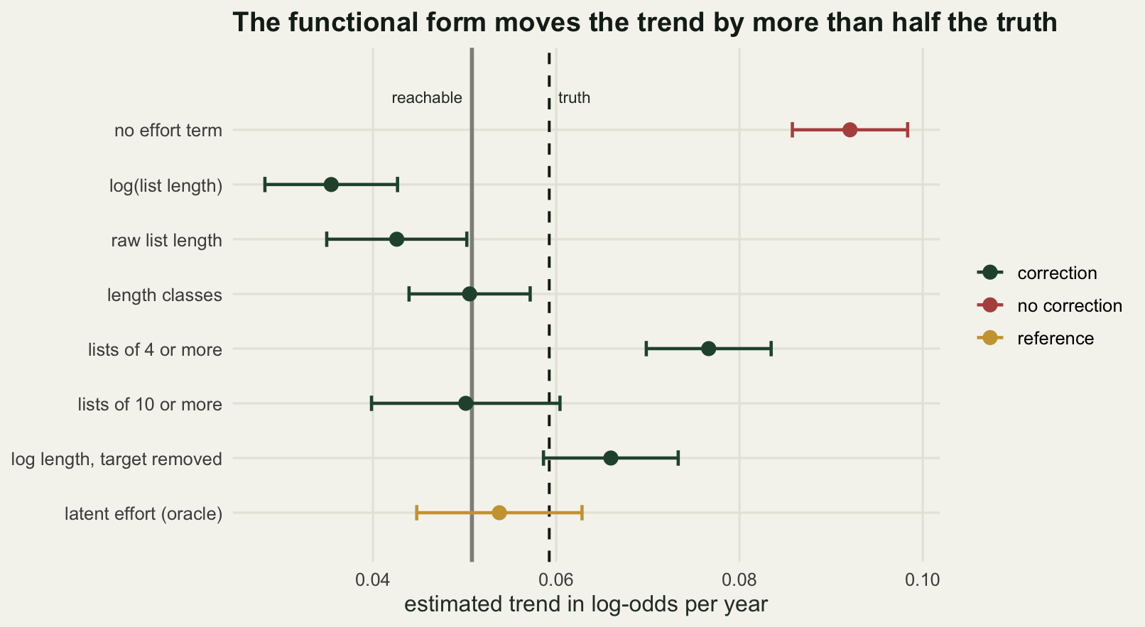
The honest limit: when list length and the species share a cause
Conditioning on list length works when list length is a proxy for effort and effort is the only thing that has changed. Two departures from that break it, and they break it in different ways.
The first is a common cause. Sites that hold more background species also hold the target more often, so list length carries site quality as well as effort. Once effort drifts, a fixed list length in a late year implies a poorer site than the same list length in an early year, and the model reads that as a fall in the species. Sweeping the strength of the site-quality effect on the target from zero to one while recomputing the truth at each step measures how fast that eats the correction.
The second is a drift that list length cannot see. Suppose the observers get better at recognising this one plant, and no better at anything else. The target’s detection rises exactly as before, but lists do not lengthen, so there is no signal for the covariate to use. The sweep below holds the total drift in the target’s detection fixed at 0.11 log-odds per year and moves it from fully shared with the other species, and so visible in list length, to fully private to the target.
set.seed(20260802)
n_sub <- 12
share_grid <- c(0, 0.25, 0.5, 0.75, 1)
shared_cause <- t(sapply(share_grid, function(s) {
  r <- t(sapply(1:n_sub, function(i) {
    dd <- sim_stream(sqt = s)
    c(unname(coef(naive_lists(dd))[2]),
      unname(coef(glm(target ~ year + lcat(listlen), binomial, dd))[2]))
  }))
  c(site_quality_effect = s, truth = true_slope(s),
    no_correction = mean(r[, 1]), corrected = mean(r[, 2]))
}))
print(round(shared_cause, 4))
site_quality_effect truth no_correction corrected
[1,] 0.00 0.0600 0.0926 0.0574
[2,] 0.25 0.0592 0.0914 0.0489
[3,] 0.50 0.0571 0.0945 0.0479
[4,] 0.75 0.0540 0.0862 0.0371
[5,] 1.00 0.0505 0.0867 0.0323invisible_grid <- c(0, 0.25, 0.5, 0.75, 1)
hidden_drift <- t(sapply(invisible_grid, function(p) {
r <- t(sapply(1:n_sub, function(i) {
dd <- sim_stream(eff_slope = eff_drift * p,
skill_slope = eff_drift * (1 - p))
c(unname(coef(naive_lists(dd))[2]),
unname(coef(glm(target ~ year + lcat(listlen), binomial, dd))[2]),
mean(dd$listlen))
}))
c(hidden_share = 1 - p, truth = b_marg, no_correction = mean(r[, 1]),
corrected = mean(r[, 2]), mean_list_length = mean(r[, 3]))
}))
print(round(hidden_drift, 4)) hidden_share truth no_correction corrected mean_list_length
[1,] 1.00 0.0592 0.0953 0.0967 8.2673
[2,] 0.75 0.0592 0.0976 0.0880 8.4480
[3,] 0.50 0.0592 0.0968 0.0756 8.6509
[4,] 0.25 0.0592 0.0950 0.0625 8.9014
[5,] 0.00 0.0592 0.0954 0.0524 9.1626site_pick <- t(sapply(c(0.04, 0.08, 0.15), function(s) {
r <- t(sapply(1:n_sub, function(i) {
dd <- sim_stream(eff_slope = 0, site_slope = s)
c(unname(coef(naive_lists(dd))[2]),
unname(coef(glm(target ~ year + lcat(listlen), binomial, dd))[2]),
mean(dd$listlen[dd$year > 4.5]) - mean(dd$listlen[dd$year < -4.5]))
}))
c(site_drift = s, no_correction = mean(r[, 1]), corrected = mean(r[, 2]),
list_length_change = mean(r[, 3]))
}))
print(round(site_pick, 4)) site_drift no_correction corrected list_length_change
[1,] 0.04 0.0579 0.0541 0.8814
[2,] 0.08 0.0665 0.0582 1.6464
[3,] 0.15 0.0821 0.0649 3.1656c(replicates_per_level = n_sub)replicates_per_level
12 The shared cause is corrosive and quiet. With no site-quality effect on the target the length-class model returns 0.0574 against a truth of 0.06. Turn the coupling up to one and it returns 0.0323 against a truth of 0.0505, so in this run an error of under three thousandths has grown to one of nearly two hundredths, and nothing in the model output changes to announce it. The uncorrected estimate barely moves across the same sweep, running between 0.0862 and 0.0945, so the usual sanity check of comparing the corrected estimate against the uncorrected one gives no warning at all.
The hidden drift is the more obvious failure and the easier one to reason about. When none of the drift shows up in list length, the corrected estimate is 0.0967 and the uncorrected one is 0.0953: the covariate has nothing to work with, and the correction does nothing. That failure does leave a mark in the data, because mean list length across the run is 8.2673 when the drift is entirely private to the target and 9.1626 when it is entirely shared. If lists are not getting longer and you still suspect effort drift, list-length analysis has no purchase on it.
The third block is the surprise. Observers drifting towards better sites is usually filed with the failures of the method, and here it is not one. At the strongest setting the uncorrected estimate is 0.0821 against a truth of 0.0592, while the length-class model returns 0.0649, so the correction removes most of that bias. Better sites yield longer lists, so this particular drift is visible in the covariate: mean list length rises by 3.1656 species between the first and last five years even though effort per visit is constant. Whether list length sees a drift is a question about that drift, not a general property of site selection, and the next post in the cluster takes the four kinds of drift apart on exactly that basis.
pan <- c("Site quality drives both list length and occupancy",
         "Drift confined to the target species")
mk <- function(m, x, lab) data.frame(
  x = rep(m[, x], 3), panel = lab,
  val = c(m[, "truth"], m[, "no_correction"], m[, "corrected"]),
  what = rep(c("true trend", "no effort term", "length classes"),
             each = nrow(m)))
lim_df <- rbind(mk(shared_cause, "site_quality_effect", pan[1]),
                mk(hidden_drift, "hidden_share", pan[2]))
lim_df$panel <- factor(lim_df$panel, levels = pan)
lim_df$what <- factor(lim_df$what,
                      levels = c("true trend", "no effort term", "length classes"))

ggplot(lim_df, aes(x, val, colour = what)) +
  geom_line(linewidth = 1) +
  geom_point(size = 2.4) +
  facet_wrap(~panel) +
  scale_colour_manual(values = c(`true trend` = te_pal$ink,
                                 `no effort term` = te_pal$clay,
                                 `length classes` = te_pal$forest), name = NULL) +
  scale_y_continuous(limits = c(0, 0.105)) +
  labs(x = "strength of the mechanism the covariate cannot handle",
       y = "estimated trend in log-odds per year",
       title = "Both failures are silent in the model output") +
  theme_te() +
  theme(legend.position = "right",
        panel.spacing.x = grid::unit(1.8, "lines"),
        strip.text = element_text(colour = te_pal$ink, face = "bold", size = 9))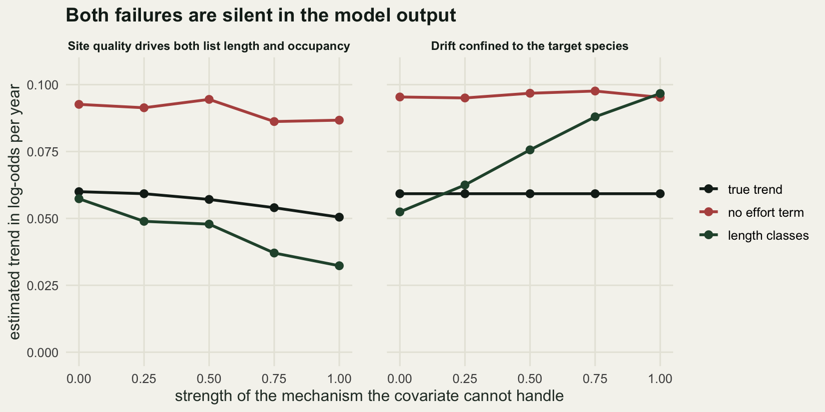
Three limits are worth stating beyond what the sweeps cover. The trend recovered is a trend in reporting, not in occupancy, and the attenuation measured earlier at 0.8582 depends on a detection probability that is itself unknown in any real dataset. The effort response was well behaved here, with an interaction of -0.0818 between log list length and period, but that is a fact about a simulator in which effort is one number acting the same way on every species, and real recording effort is several things at once. And the whole exercise conditions on a list being submitted at all, so anything that changes which visits get written up, rather than what appears on them once they are, sits outside the model entirely.
Where to go next
The obvious complaint about everything above is that it estimates a reporting trend and then apologises for the difference. The way out is to stop treating each list as an independent trial and start building detection histories, which is what occupancy from unstructured records does with the same kind of record stream: the likelihood is the standard one from single-season occupancy model, and only the data preparation changes. That buys the separation of occupancy from detection at the price of a new set of arbitrary decisions about what counts as a repeat visit.
Before that, it is worth knowing how large the effort problem can get and which flavours of it the list-length covariate can see, which is measured directly in reporting rates and effort drift. The site-selection result above is a preview: not every effort drift is invisible to a list-length model, and the ones that are invisible are the ones to worry about.
References
MacKenzie DI, Nichols JD, Lachman GB, Droege S, Royle JA, Langtimm CA 2002 Ecology 83(8):2248-2255 (10.1890/0012-9658(2002)083[2248:ESORWD]2.0.CO;2)
Szabo JK, Vesk PA, Baxter PWJ, Possingham HP 2010 Ecological Applications 20(8):2157-2169 (10.1890/09-0877.1)
Hill MO 2012 Methods in Ecology and Evolution 3(1):195-205 (10.1111/j.2041-210X.2011.00146.x)
van Strien AJ, van Swaay CAM, Termaat T 2013 Journal of Applied Ecology 50(6):1450-1458 (10.1111/1365-2664.12158)
Isaac NJB, van Strien AJ, August TA, de Zeeuw MP, Roy DB 2014 Methods in Ecology and Evolution 5(10):1052-1060 (10.1111/2041-210X.12254)