library(ggplot2)
library(patchwork)

te_paper  <- "#f5f4ee"
te_ink    <- "#16241d"
te_body   <- "#2c3a31"
te_forest <- "#275139"
te_rust   <- "#b5534e"
te_gold   <- "#c9b458"
te_line   <- "#dad9ca"

theme_datasheet <- function() {
  theme_minimal(base_size = 12) +
    theme(plot.background  = element_rect(fill = te_paper, colour = NA),
          panel.background = element_rect(fill = te_paper, colour = NA),
          panel.grid.major = element_line(colour = te_line, linewidth = 0.3),
          panel.grid.minor = element_blank(),
          text             = element_text(colour = te_body),
          plot.title       = element_text(colour = te_ink, face = "bold"),
          plot.subtitle    = element_text(colour = te_body),
          axis.text        = element_text(colour = te_body))
}Snapped coordinates and a clustering verdict
R
point patterns
spatial ecology
occurrence data
data cleaning
ecology tutorial
Records stored at grid centroids make a random pattern look clustered, and one record per cell makes it look regular. Measuring both in R with Clark-Evans.
An orchid atlas has three hundred records from a square block of hill country, all entered as grid references, so each record carries the centre of its grid square rather than the spot where the plant grew. The first analysis anyone runs on such a set is a test of whether the plants are aggregated, and the first test in most courses is the Clark-Evans index: the mean distance from each record to its nearest neighbour, divided by what that mean would be if the records were scattered at random. The index comes back well below one, the simulation envelope agrees, and the report says the orchid is clustered.
A reviewer points out that many records sit on exactly the same coordinates and asks for duplicates to be removed, which is standard advice in occurrence-cleaning workflows. One record per grid cell is kept, the index is rerun, and it now comes back well above one: the orchid is regular. Nothing about the orchid changed between the two runs. What changed is how its coordinates were stored and then tidied.
This post measures both steps on patterns whose truth is known. Nearest-neighbour analysis and Clark-Evans in R builds the index on clean simulated points, and its closing section on what nearest neighbours miss is about scale, not about ties. Checking a point pattern analysis shows random maps being called clustered, but there the cause is how the envelope is read, on coordinates that are exact; its honest limits name inhomogeneity, not coordinate storage, as the remaining threat. Cleaning GBIF and iNaturalist records in R runs the duplicate step and filters on stated coordinate precision, and reports how many rows each step removes, without asking what either does to an analysis further down.
The closest measurement already on this site is in Sampling bias in presence-only models. Its section on spatial thinning shows one record per cell pulling a species distribution slope well below the truth, at a correlation where the unthinned fit was already right. This post is the same clean-up step read by a distance statistic instead of a regression slope, and the damage is of a different kind: there it changes the environmental make-up of the retained sample, here it changes the geometry, and it pushes the statistic in the opposite direction from the one the raw records pushed it. Coordinate error and habitat assignment is the other near relative, and the difference is worth stating once. Coordinate error moves a record; a coordinate grid puts many records in the same place, and a nearest-neighbour statistic cannot tell an aggregation from a shared cell.
The index is Clark and Evans (1954). The cleaning steps being measured are the ones automated by CoordinateCleaner (Zizka and colleagues 2019) and argued for by Maldonado and colleagues (2015), and the envelopes follow Baddeley, Rubak and Turner (2015). None of those sources claims the reversal measured below; it is the measured piece here, not a published result.
The index, the envelope and the storage grid
The window is a square of side 100 units holding 300 records, so a unit can be read as a tenth of a kilometre and the square as a ten kilometre atlas block. Storage on a grid of cell size h replaces every coordinate by the centre of the cell it falls in, which is what a grid reference, a rounded decimal degree or a site centroid does. Cell sizes of 1, 2, 5 and 10 units divide the side exactly, so every cell is whole. The clean-up keeps the first record at each distinct stored location.
The Clark-Evans index here is the naive one: observed mean nearest-neighbour distance over the complete spatial randomness expectation of one over twice the square root of the density, with no edge correction. That choice is deliberate, because it is what most scripts compute, and it has a consequence that has to be handled before anything else. Without an edge correction the index on random points sits above one, so a verdict read against the nominal value of one would be biased before the coordinates were touched. Every verdict below is read against a simulation envelope built with the same statistic: the 2.5 and 97.5 per cent quantiles of the index over 199 random patterns of the same size, with exact coordinates, which is the envelope an analyst would actually build.
side    <- 100
area    <- side^2
n_rec   <- 300
n_env   <- 199
cells_h <- c(0, 1, 2, 5, 10)

nn_dist <- function(x, y) {
  d2 <- outer(x, x, "-")^2 + outer(y, y, "-")^2
  diag(d2) <- Inf
  sqrt(d2[cbind(seq_along(x), max.col(-d2, ties.method = "first"))])
}
ce_expect <- function(n_pts) 1 / (2 * sqrt(n_pts / area))
ce_index  <- function(x, y) mean(nn_dist(x, y)) / ce_expect(length(x))

csr_pts  <- function(n_pts) list(x = runif(n_pts, 0, side), y = runif(n_pts, 0, side))
snap_pts <- function(pts, h) {
  if (h == 0) return(pts)
  list(x = (floor(pts$x / h) + 0.5) * h, y = (floor(pts$y / h) + 0.5) * h)
}
one_per_cell <- function(pts) {
  keep <- !duplicated(paste(pts$x, pts$y))
  list(x = pts$x[keep], y = pts$y[keep])
}

env_store <- new.env()
env_exact <- function(n_pts) {
  key <- as.character(n_pts)
  if (is.null(env_store[[key]])) {
    sims <- replicate(n_env, { q <- csr_pts(n_pts); ce_index(q$x, q$y) })
    env_store[[key]] <- quantile(sims, c(0.025, 0.975), names = FALSE)
  }
  env_store[[key]]
}
call_it <- function(r_val, band) {
  ifelse(r_val < band[1], "clustered", ifelse(r_val > band[2], "regular", "random"))
}

set.seed(2501)
env_300  <- env_exact(n_rec)
mean_nn0 <- ce_expect(n_rec)
At this density the random expectation of the nearest-neighbour distance is 2.89 units, so a cell of 5 units is 1.7 times the typical spacing between records and a cell of 2 units is 0.69 times it. The envelope for 300 exact random points runs from 0.966 to 1.081. It is not centred on one, and that is the edge effect: a record near the boundary has its true nearest neighbour outside the window, unobserved, so its measured distance is too long.
A random map, stored on a grid, is called clustered
Each of 100 fresh random patterns is stored at every cell size, including a cell size of zero, which is the unrounded control. The index and the share of records whose nearest neighbour sits at distance exactly zero are recorded, and the verdict is read against the envelope above. The same stored pattern is then cleaned to one record per cell, the index is recomputed at the reduced number of records, and its verdict is read against a fresh envelope built at that reduced number.
n_draw <- 100
set.seed(3251)
sim_rows <- vector("list", n_draw * length(cells_h))
row_i <- 0
for (d_i in seq_len(n_draw)) {
  pts0 <- csr_pts(n_rec)
  for (h in cells_h) {
    stored  <- snap_pts(pts0, h)
    nn_st   <- nn_dist(stored$x, stored$y)
    r_raw   <- mean(nn_st) / mean_nn0
    cleaned <- one_per_cell(stored)
    n_kept  <- length(cleaned$x)
    nn_cl   <- nn_dist(cleaned$x, cleaned$y)
    r_clean <- mean(nn_cl) / ce_expect(n_kept)
    row_i <- row_i + 1
    sim_rows[[row_i]] <- data.frame(
      draw = d_i, h = h, r_raw = r_raw, zero_share = mean(nn_st == 0),
      raw_call = call_it(r_raw, env_300), n_kept = n_kept, r_clean = r_clean,
      min_nn_clean = min(nn_cl), clean_call = call_it(r_clean, env_exact(n_kept)),
      clean_call_300 = call_it(r_clean, env_300))
  }
}
sim_res <- do.call(rbind, sim_rows)

zero_theory <- function(h) ifelse(h == 0, 0, 1 - (1 - h^2 / area)^(n_rec - 1))
kept_theory <- function(h) ifelse(h == 0, n_rec, (area / h^2) * (1 - (1 - h^2 / area)^n_rec))

share_se <- function(p) sqrt(p * (1 - p) / n_draw)
by_h <- do.call(rbind, lapply(cells_h, function(h) {
  s <- sim_res[sim_res$h == h, ]
  data.frame(
    h = h, r_raw = median(s$r_raw), r_raw_lo = min(s$r_raw), r_raw_hi = max(s$r_raw),
    zero_share = mean(s$zero_share), zero_pred = zero_theory(h),
    raw_clustered = mean(s$raw_call == "clustered"), raw_regular = mean(s$raw_call == "regular"),
    n_kept = mean(s$n_kept), kept_pred = kept_theory(h),
    r_clean = median(s$r_clean), r_clean_lo = min(s$r_clean), r_clean_hi = max(s$r_clean),
    clean_regular = mean(s$clean_call == "regular"),
    clean_clustered = mean(s$clean_call == "clustered"),
    clean_regular_300 = mean(s$clean_call_300 == "regular"))
}))
row_of <- function(h) by_h[by_h$h == h, ]
ctl <- row_of(0); h1 <- row_of(1); h2 <- row_of(2); h5 <- row_of(5); h10 <- row_of(10)
ctl_out <- ctl$raw_clustered + ctl$raw_regular
of_n <- function(p) sprintf("%d of %d", round(p * n_draw), n_draw)
tab_show <- data.frame(
cell = ifelse(by_h$h == 0, "0 (unrounded control)", sprintf("%d", by_h$h)),
R_stored = sprintf("%.3f (%.3f to %.3f)", by_h$r_raw, by_h$r_raw_lo, by_h$r_raw_hi),
zero_nn = sprintf("%.3f", by_h$zero_share),
called_clustered = sprintf("%.2f", by_h$raw_clustered),
kept = sprintf("%.1f", by_h$n_kept),
R_one_per_cell = sprintf("%.3f (%.3f to %.3f)", by_h$r_clean, by_h$r_clean_lo, by_h$r_clean_hi),
called_regular = sprintf("%.2f", by_h$clean_regular))
knitr::kable(tab_show, align = "lllrrlr",
col.names = c("cell size", "R as stored, median (range)", "share of zero NN distances",
"share called clustered", "records kept", "R one per cell, median (range)",
"share called regular"))| cell size | R as stored, median (range) | share of zero NN distances | share called clustered | records kept | R one per cell, median (range) | share called regular |
|---|---|---|---|---|---|---|
| 0 (unrounded control) | 1.029 (0.959 to 1.098) | 0.000 | 0.02 | 300.0 | 1.029 (0.959 to 1.098) | 0.05 |
| 1 | 1.026 (0.962 to 1.096) | 0.027 | 0.05 | 295.9 | 1.048 (0.985 to 1.120) | 0.11 |
| 2 | 1.019 (0.931 to 1.085) | 0.113 | 0.07 | 282.8 | 1.115 (1.051 to 1.187) | 0.81 |
| 5 | 0.853 (0.719 to 0.989) | 0.521 | 0.99 | 212.2 | 1.500 (1.441 to 1.538) | 1.00 |
| 10 | 0.162 (0.092 to 0.277) | 0.952 | 1.00 | 94.9 | 1.949 (1.887 to 1.990) | 1.00 |
set.seed(9090)
env_check    <- replicate(2000, { q <- csr_pts(n_rec); ce_index(q$x, q$y) })
env_true_out <- mean(env_check < env_300[1] | env_check > env_300[2])
The control row behaves as it should. Unrounded random patterns give a median index of 1.029, inside their own envelope, and 7 of 100 draws fall outside it, against a nominal five in a hundred (Monte Carlo standard error 0.022 on the share). The excess is the envelope itself: against 2000 further random patterns of 300 records, this 199-pattern band excludes a share of 0.070, not 0.05, because a quantile taken from 199 patterns is itself noisy and this one came out slightly narrow. The stored-record verdicts at every cell size are read against the same band and carry the same small excess. With that allowed for, the statistic and the envelope agree with each other before any storage grid is applied.
At a cell of 5 units the median index of the stored records is 0.853 and 99 of 100 draws are called clustered. The reason is in the next column: 0.521 of the records have a nearest neighbour at distance exactly zero, because they share a cell with at least one other record. At a cell of 10 units the zero share is 0.952, the median index collapses to 0.162 and 100 of 100 draws are called clustered. At 1 and 2 units the stored records are still read almost correctly: 5 of 100 and 7 of 100 draws are called clustered, against 2 of 100 for the control and a nominal 2.5 in a hundred on that side, so a small excess at most (standard error 0.026 at 2 units), and nothing like the cell of 5, although 0.113 of records already have a zero distance at 2 units.
The zero share is the one quantity here that follows from a formula. A record has a zero nearest-neighbour distance exactly when at least one of the other 299 records falls in its cell, so its expected share is one minus (1 minus h squared over the area) to the power 299. That gives 0.113, 0.527 and 0.950 at 2, 5 and 10 units, against simulated shares of 0.113, 0.521 and 0.952. The formula calibrates the snap; it does not give the index, and it does not give the verdict, which also depends on how the non-zero distances shift and on the envelope.
h_curve <- data.frame(h = seq(0.25, 10.5, by = 0.05))
h_curve$zero <- zero_theory(h_curve$h)
h_curve$kept <- kept_theory(h_curve$h)
pts_cal <- by_h[by_h$h > 0, ]
cal_zero <- ggplot(h_curve, aes(h, zero)) +
  geom_line(colour = te_gold, linewidth = 1) +
  geom_point(data = pts_cal, aes(h, zero_share), colour = te_forest, size = 2.8) +
  labs(x = "cell size (units)", y = "share of zero NN distances",
       title = "Records sharing a cell") +
  theme_datasheet()
cal_kept <- ggplot(h_curve, aes(h, kept)) +
  geom_line(colour = te_gold, linewidth = 1) +
  geom_point(data = pts_cal, aes(h, n_kept), colour = te_rust, size = 2.8) +
  labs(x = "cell size (units)", y = "records kept after cleaning",
       title = "Records left by one per cell") +
  theme_datasheet()
(cal_zero | cal_kept) +
  plot_annotation(subtitle = "gold line: occupancy formula; points: mean of 100 simulated patterns",
                  theme = theme_datasheet())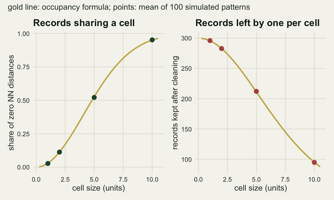
set.seed(77)
ex_csr   <- csr_pts(n_rec)
thomas_pts <- function(n_parent = 30, per_parent = 10, spread = 3) {
  px <- runif(n_parent, 0, side); py <- runif(n_parent, 0, side)
  x <- rep(px, each = per_parent) + rnorm(n_parent * per_parent, 0, spread)
  y <- rep(py, each = per_parent) + rnorm(n_parent * per_parent, 0, spread)
  inside <- x > 0 & x < side & y > 0 & y < side
  list(x = x[inside], y = y[inside])
}
ex_thomas <- thomas_pts()

stage_frame <- function(pts, lab_pattern) {
  stored  <- snap_pts(pts, 5)
  key     <- paste(stored$x, stored$y)
  counts  <- as.vector(table(key)[key])
  cleaned <- one_per_cell(stored)
  rbind(
    data.frame(x = pts$x, y = pts$y, n_here = 1, stage = "exact coordinates"),
    data.frame(x = stored$x, y = stored$y, n_here = counts, stage = "stored on a 5 unit grid")[!duplicated(key), ],
    data.frame(x = cleaned$x, y = cleaned$y, n_here = 1, stage = "one record per cell")) |>
    transform(pattern = lab_pattern)
}
map_df <- rbind(stage_frame(ex_csr, "random"), stage_frame(ex_thomas, "clustered (Thomas)"))
map_df$stage   <- factor(map_df$stage, levels = c("exact coordinates", "stored on a 5 unit grid",
                                                  "one record per cell"))
map_df$pattern <- factor(map_df$pattern, levels = c("random", "clustered (Thomas)"))ggplot(map_df, aes(x, y)) +
geom_point(aes(size = n_here), colour = te_forest, alpha = 0.75, stroke = 0) +
scale_size_area(max_size = 3.2, breaks = c(1, 3, 6), name = "records at the point") +
facet_grid(pattern ~ stage) +
coord_equal(xlim = c(0, side), ylim = c(0, side), expand = FALSE) +
labs(x = NULL, y = NULL, title = "What the storage grid does to the map") +
theme_datasheet() +
theme(axis.text = element_blank(), legend.position = "bottom",
panel.border = element_rect(colour = te_line, fill = NA),
strip.text = element_text(colour = te_ink))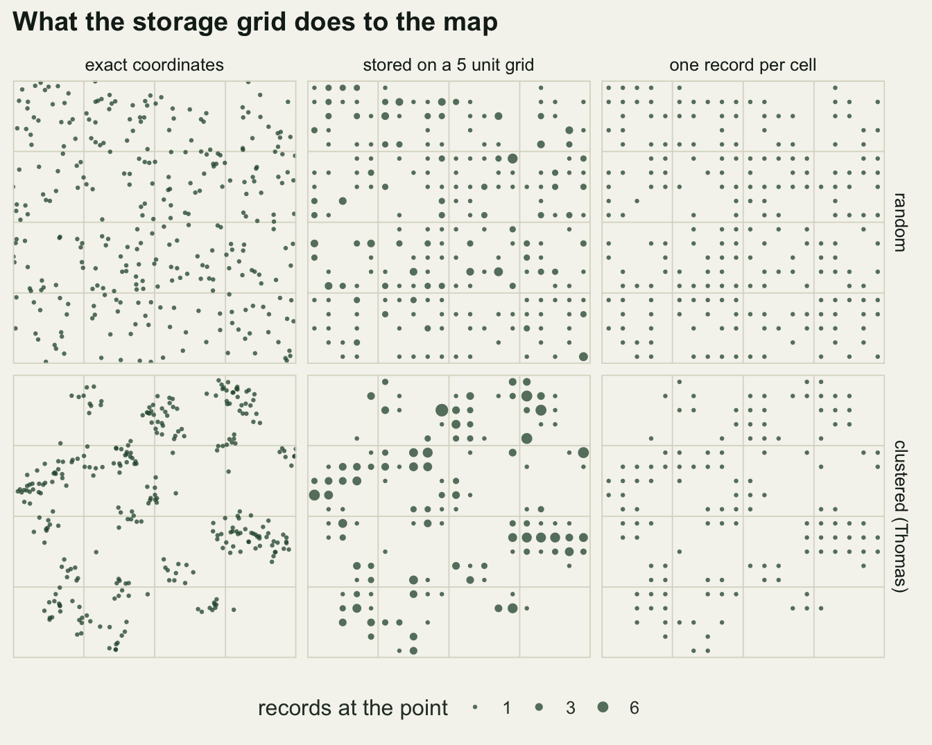
One record per cell turns the verdict round
Cleaning the same stored records to one per cell reverses the call. At 5 units the number of records falls from 300 to 212.2 on average (the occupancy formula, the number of cells times the chance a cell holds at least one record, gives 211.2), the median index rises to 1.500, and 100 of 100 draws are called regular. At 10 units, with 94.9 records kept, the median is 1.949 and 100 of 100 draws are called regular.
lower_bound <- 2 * sim_res$h * sqrt(sim_res$n_kept / area)
above_bound <- mean((sim_res$r_clean >= lower_bound - 1e-9)[sim_res$h > 0])
bound_h5    <- median(lower_bound[sim_res$h == 5])
bound_h10   <- median(lower_bound[sim_res$h == 10])
min_nn_h5   <- min(sim_res$min_nn_clean[sim_res$h == 5])
env_hi_h2   <- median(vapply(sim_res$n_kept[sim_res$h == 2], function(k) env_exact(k)[2], 0))
bound_h1    <- median(lower_bound[sim_res$h == 1])
bound_h2    <- median(lower_bound[sim_res$h == 2])
at_floor_h10 <- mean(abs(sim_res$r_clean - lower_bound)[sim_res$h == 10] < 1e-9)
short_nn_h2 <- 1 - exp(-pi * h2$n_kept / area * 2^2)
The mechanism is geometric. After the clean-up every record sits at the centre of a different cell, so the pattern is a subset of a lattice and no two records can be closer than one cell width: the smallest nearest-neighbour distance in any cleaned 5 unit pattern is 5.00. The index therefore cannot fall below the cell size over the random expectation at the reduced count, two h times the square root of the kept count over the area. At 5 and 10 units that floor alone settles the verdict. At 5 units it has a median of 1.459 across draws, already far above any envelope, and at 10 units it is 1.949, and there the cleaned index equals its floor in 98 of 100 draws, the ones in which every record’s nearest neighbour is exactly one cell away; with 94.9 of 100 cells occupied on average, an occupied cell with no occupied cell directly beside it is rare. Across all draws at the four cell sizes the cleaned index sits on or above its floor in a share of 1.000 of cases, which is a check on the code rather than a finding. The raw records were read by a statistic with an atom at zero; the cleaned ones are read by a statistic with a lower bound far from zero.
The finer end of the table is the sharper half of the finding. At 2 units the stored records are read almost correctly, as noted above, but after cleaning 81 of 100 draws are called regular (standard error of the share 0.039), with a median index of 1.115. The clean-up bites at a finer cell than the rounding does. Even at 1 unit, a tenth of a kilometre in the atlas reading, 11 of 100 cleaned draws are called regular, against 5 of 100 for the unrounded control.
Reading the cleaned index against the original envelope for 300 points, which is what happens when a script builds its envelope once from the raw record count, moves the counts to 86 of 100 at 2 units and 14 of 100 at 1 unit. The upper limit of the envelope for 300 points is 1.081, and the median upper limit of the envelopes at the reduced counts for 2 units is 1.090. That difference is of the order of the simulation noise in an envelope quantile from 199 patterns, so building the envelope at the wrong count adds a little to the error here but is not its source. Nor is the floor at this cell size: its median is 0.673 at 2 units and 0.344 at 1 unit, far below the envelope. What moves the index at the fine end is the minimum spacing itself. Among exact random points at the cleaned count for 2 units, about 0.30 of nearest-neighbour distances are shorter than 2 units (the Poisson nearest-neighbour formula, one minus e to the power of minus pi times the density times the squared distance), and after cleaning none can be.
long_r <- rbind(
  data.frame(h = sim_res$h, r_val = sim_res$r_raw, step = "as stored, 300 records"),
  data.frame(h = sim_res$h, r_val = sim_res$r_clean, step = "one record per cell"))
long_r$step <- factor(long_r$step, levels = c("as stored, 300 records", "one record per cell"))
env_df <- do.call(rbind, lapply(cells_h, function(h) {
  med_n <- round(median(sim_res$n_kept[sim_res$h == h]))
  rbind(data.frame(h = h, lo = env_300[1], hi = env_300[2], step = "as stored, 300 records"),
        data.frame(h = h, lo = env_exact(med_n)[1], hi = env_exact(med_n)[2],
                   step = "one record per cell"))
}))
env_df$step <- factor(env_df$step, levels = levels(long_r$step))
h_lab <- function(v) factor(ifelse(v == 0, "0 (exact)", as.character(v)),
                            levels = c("0 (exact)", "1", "2", "5", "10"))
long_r$h_f <- h_lab(long_r$h); env_df$h_f <- h_lab(env_df$h)

ggplot(long_r, aes(h_f, r_val)) +
  geom_tile(data = env_df, aes(x = h_f, y = (lo + hi) / 2, height = hi - lo),
            inherit.aes = FALSE, fill = te_gold, colour = te_gold, alpha = 0.45, width = 0.7) +
  geom_jitter(aes(colour = step), width = 0.18, height = 0, size = 1.1, alpha = 0.6) +
  scale_colour_manual(values = c(te_forest, te_rust), guide = "none") +
  facet_wrap(~ step) +
  labs(x = sprintf("cell size of the storage grid (units; random spacing of 300 records is %.2f)", mean_nn0),
       y = "Clark-Evans index, naive",
       title = "The same records, called clustered and then regular",
       subtitle = "gold boxes: 2.5 to 97.5 per cent envelope of exact random points at the same count") +
  theme_datasheet() +
  theme(strip.text = element_text(colour = te_ink, face = "bold"))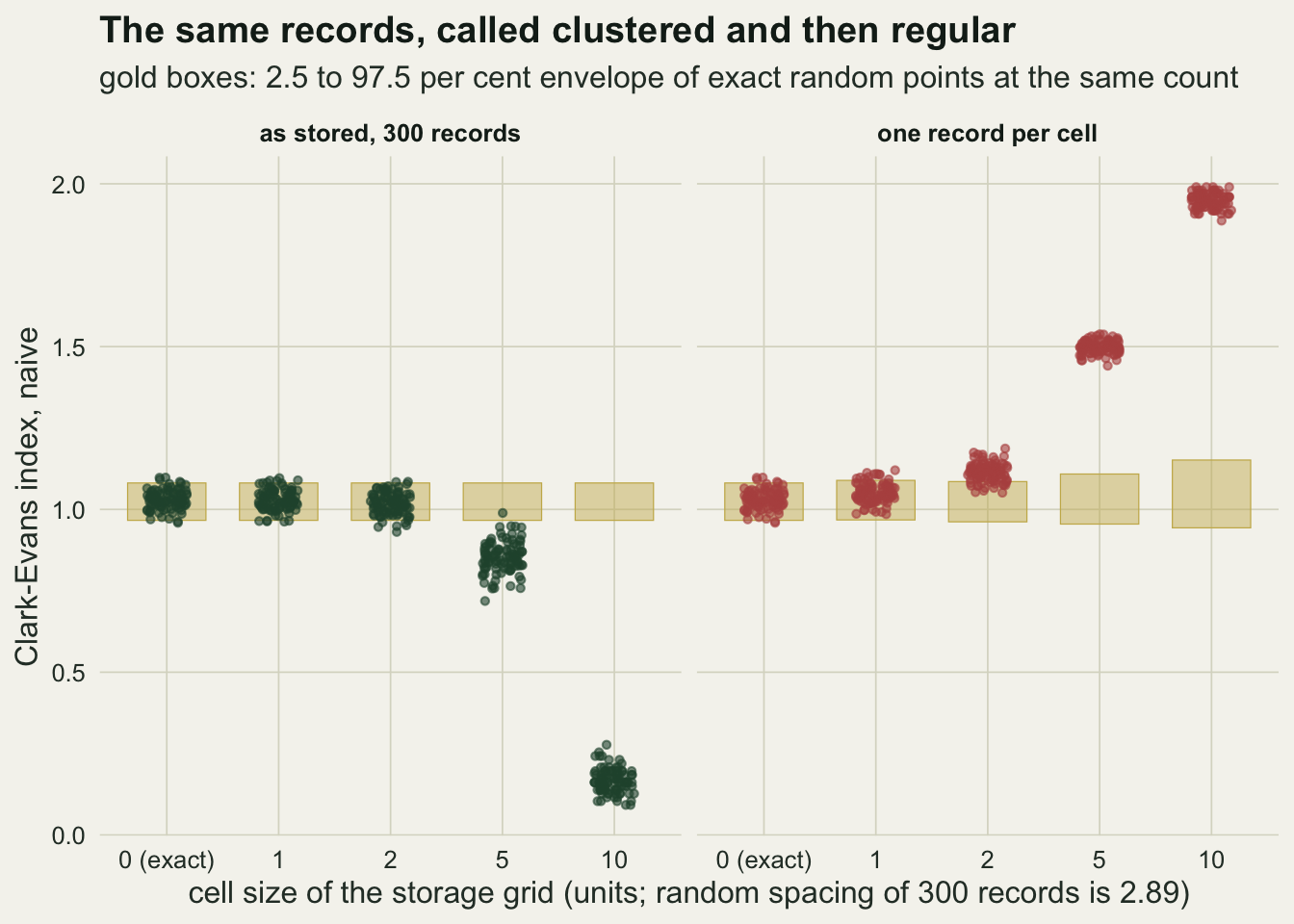
A real clustering verdict does not survive the same two steps
The first two sections manufacture a pattern where there is none. The more damaging case runs the other way. A Thomas cluster process places 30 parent points at random and 10 offspring around each with a normal spread of 3 units, and offspring falling outside the window are dropped. This is a pattern that is clustered by construction, with a spread of the same order as the 5 unit cell. It goes through the same storage grid and the same clean-up.
set.seed(6060)
th_rows <- vector("list", n_draw)
for (d_i in seq_len(n_draw)) {
  pts0   <- thomas_pts()
  n0     <- length(pts0$x)
  r0     <- ce_index(pts0$x, pts0$y)
  stored <- snap_pts(pts0, 5)
  nn_st  <- nn_dist(stored$x, stored$y)
  r_st   <- mean(nn_st) / ce_expect(n0)
  cleaned <- one_per_cell(stored)
  n_kept  <- length(cleaned$x)
  r_cl    <- ce_index(cleaned$x, cleaned$y)
  th_rows[[d_i]] <- data.frame(
    n0 = n0, r0 = r0, call0 = call_it(r0, env_exact(n0)),
    r_st = r_st, zero_share = mean(nn_st == 0), call_st = call_it(r_st, env_exact(n0)),
    n_kept = n_kept, r_cl = r_cl, call_cl = call_it(r_cl, env_exact(n_kept)))
}
th_res <- do.call(rbind, th_rows)
th_sum <- list(
  n0 = median(th_res$n0), r0 = median(th_res$r0), clu0 = mean(th_res$call0 == "clustered"),
  r_st = median(th_res$r_st), zero = mean(th_res$zero_share),
  clu_st = mean(th_res$call_st == "clustered"),
  n_kept = median(th_res$n_kept), r_cl = median(th_res$r_cl),
  clu_cl = mean(th_res$call_cl == "clustered"), rnd_cl = mean(th_res$call_cl == "random"),
  reg_cl = mean(th_res$call_cl == "regular"))
With exact coordinates the pattern is read correctly: a median of 287 records survive the window, the median index is 0.596, and 100 of 100 draws are called clustered. Storing the records on the 5 unit grid exaggerates the clustering, since offspring of one parent tend to share cells: the zero share is 0.814 and the median index drops to 0.317. The clean-up then leaves a median of 127 records, the median index is 1.134, and 0 of 100 draws are called clustered: 55 are called random and 45 regular.
The six maps above (the second figure) show why this is not a failure to detect something faint. The cleaned Thomas pattern is still visibly a set of tight patches of occupied cells separated by empty ground. What the patches no longer have is short distances inside them, and the nearest-neighbour index looks at nothing else.
An envelope on the storage grid
The repair a spatial statistician would suggest is to build the null on the same support as the data: simulate random points, then apply the same grid and the same clean-up, so the envelope carries the atom at zero and the lattice floor as well. For stored records that means random patterns of 300 points snapped to the grid. For cleaned records there is a simpler exact form. Under complete spatial randomness every cell is equally likely to be occupied, so given the number of occupied cells, the set of occupied cells is a random subset of the grid of that size; the envelope comes from drawing that many cells at random without replacement and placing a record at each centre. This conditions on the count the analyst actually has after cleaning, and needs no knowledge of how many records there were before.
set.seed(4747)
grid_env_store <- new.env()
env_grid <- function(h, n_occ) {
  key <- paste(h, n_occ)
  if (is.null(grid_env_store[[key]])) {
    k_side <- side / h
    sims <- replicate(n_env, {
      cell_id <- sample.int(k_side * k_side, n_occ)
      ce_index(((cell_id - 1) %% k_side + 0.5) * h, ((cell_id - 1) %/% k_side + 0.5) * h)
    })
    grid_env_store[[key]] <- quantile(sims, c(0.025, 0.975), names = FALSE)
  }
  grid_env_store[[key]]
}
env_snapped <- lapply(c(2, 5, 10), function(h) {
  sims <- replicate(n_env, { q <- snap_pts(csr_pts(n_rec), h); ce_index(q$x, q$y) })
  quantile(sims, c(0.025, 0.975), names = FALSE)
})
names(env_snapped) <- c("2", "5", "10")

rep_rows <- do.call(rbind, lapply(c(2, 5, 10), function(h) {
  s <- sim_res[sim_res$h == h, ]
  raw_grid   <- call_it(s$r_raw, env_snapped[[as.character(h)]])
  clean_grid <- mapply(function(r_val, n_k) call_it(r_val, env_grid(h, n_k)), s$r_clean, s$n_kept)
  data.frame(h = h,
             raw_exact = mean(s$raw_call != "random"), raw_grid = mean(raw_grid != "random"),
             clean_exact = mean(s$clean_call != "random"), clean_grid = mean(clean_grid != "random"))
}))
th_grid_call <- mapply(function(r_val, n_k) call_it(r_val, env_grid(5, n_k)),
                       th_res$r_cl, th_res$n_kept)
th_grid_clu  <- mean(th_grid_call == "clustered")
rep_h <- function(h) rep_rows[rep_rows$h == h, ]
r2 <- rep_h(2); r5 <- rep_h(5); r10 <- rep_h(10)
worst_grid <- max(c(rep_rows$raw_grid, rep_rows$clean_grid))
On the stored records the envelope from snapped random patterns runs from 0.721 to 0.941 at 5 units, well below the exact-coordinate envelope, and the number of random patterns called non-random falls from 99 of 100 to 6 of 100. On the cleaned records the grid-subset envelope does the same in the other direction: the count called non-random at 5 units falls from 100 of 100 to 8 of 100, and at 2 units from 81 of 100 to 8 of 100. Across the three cell sizes and both steps the largest non-random share under the grid envelopes is 0.08, against a nominal 0.05, with a Monte Carlo standard error of about 0.022 at the nominal level. So the repair fixes both directions at once on random data.
The part that matters more is the clustered pattern. Against the grid-subset envelope the cleaned Thomas records are called clustered in 100 of 100 draws, where the exact-coordinate envelope gave 0 of 100. The information was not destroyed by the clean-up; it moved from the distances inside a patch to the arrangement of occupied cells, and a null built on the grid can still see it.
rep_long <- rbind(
  data.frame(case = sprintf("random, as stored, cell %d", rep_rows$h),
             exact = rep_rows$raw_exact, grid = rep_rows$raw_grid),
  data.frame(case = sprintf("random, one per cell, cell %d", rep_rows$h),
             exact = rep_rows$clean_exact, grid = rep_rows$clean_grid),
  data.frame(case = "clustered, one per cell, cell 5", exact = th_sum$clu_cl, grid = th_grid_clu))
rep_long$case <- factor(rep_long$case, levels = rev(rep_long$case))
rep_plot <- rbind(
  data.frame(case = rep_long$case, share = rep_long$exact, env = "envelope on exact coordinates"),
  data.frame(case = rep_long$case, share = rep_long$grid, env = "envelope on the storage grid"))
rep_plot$se <- share_se(rep_plot$share)

ggplot(rep_plot, aes(share, case, colour = env)) +
  geom_vline(xintercept = 0.05, linetype = "dashed", colour = te_body, linewidth = 0.5) +
  geom_errorbar(aes(xmin = pmax(share - 2 * se, 0), xmax = pmin(share + 2 * se, 1)),
                orientation = "y", width = 0.25, linewidth = 0.6,
                position = position_dodge(width = 0.55)) +
  geom_point(size = 2.6, position = position_dodge(width = 0.55)) +
  scale_colour_manual(values = c(te_rust, te_forest), name = NULL) +
  scale_x_continuous(limits = c(0, 1), breaks = seq(0, 1, 0.2)) +
  labs(x = "share of patterns given the verdict", y = NULL,
       title = "A null on the grid fixes both directions",
       subtitle = "dashed line: the nominal five per cent") +
  theme_datasheet() +
  theme(legend.position = "bottom")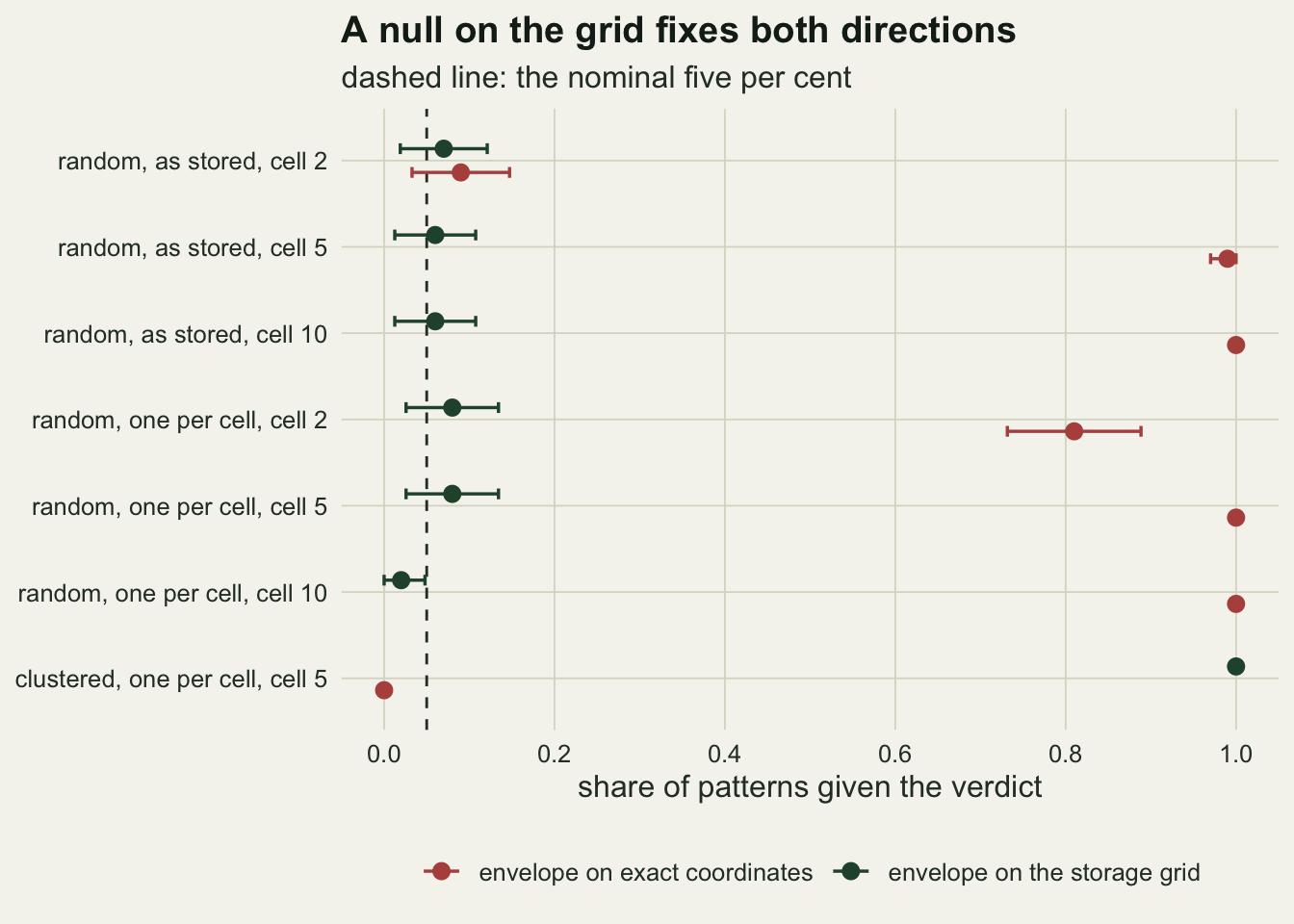
What to report
Check the storage before running any distance statistic. Two numbers do it and both are one line of R: the share of records whose nearest neighbour is at distance exactly zero, and the number of distinct values in each coordinate column.
set.seed(515)
diag_pts <- csr_pts(n_rec)
diag_tab <- do.call(rbind, lapply(cells_h, function(h) {
  st <- snap_pts(diag_pts, h)
  data.frame(cell = h, zero_nn = round(mean(nn_dist(st$x, st$y) == 0), 3),
             distinct_x = length(unique(st$x)), distinct_y = length(unique(st$y)))
}))
diag_tab
cell zero_nn distinct_x distinct_y
1 0 0.000 300 300
2 1 0.013 94 98
3 2 0.153 50 50
4 5 0.563 20 20
5 10 0.937 10 10On exact coordinates there are as many distinct values as records and no zero distances. On a 5 unit grid there are 20 distinct x values among 300 records. In a real download the same check is a count of decimal places: a coordinate with two decimal places of a degree is a grid of roughly a kilometre, and a column where most values have two decimals and a few have six is a mixture of storage grids, which no single-grid null in this post can handle (that case is not simulated here). Count the decimals on the text as downloaded, since a numeric column drops trailing zeros. A stated coordinate uncertainty, where it exists, gives the same information more directly, but the cleaning tutorial on this site keeps blank uncertainties rather than dropping them, and the decimal count works on every record. At the level of a whole dataset, CoordinateCleaner’s cd_round() automates a related check: it flags datasets whose coordinates show the periodic spacing of a lattice, as atlas data often do.
If the records are on a grid, say which grid, and build the null on it. For stored records that means simulating random points and snapping them the same way; for records cleaned to one per cell it means drawing the same number of cells at random from the grid. Report the index with that envelope, and report the zero share and the kept count next to the occupancy formula, so a reader can see the snap has been accounted for.
Do not read a Clark-Evans index from gridded records against one, and do not read it against an envelope of exact random points. The table above gives the sizes of those errors for one design. If the cleaned records are going into a species distribution model rather than a point-pattern test, the thinning section of the presence-only post is the relevant measurement, and its damage is to the slope, not to the verdict.
Honest limits
Everything is measured for 300 records in a square window, with cell sizes that divide the side exactly. A grid that does not align with the study boundary leaves partial cells at the edges, and the occupancy formula becomes an approximation there. Rounded decimal degrees are not square cells away from the equator, and a mixture of storage grids in one dataset, which is common in atlas data, was not simulated.
The statistic is the naive Clark-Evans index, chosen because it is common and because its edge bias forced the envelopes to be built honestly. An edge-corrected index would move the control row towards one but would not change the atom at zero or the lattice floor, which are the mechanisms here. The pair correlation function at short distances would show the ties even more plainly, as a spike at zero, and Ripley’s K would inherit them at every distance; neither was measured.
The clustered case is one Thomas process with a cluster spread of 3 units against a 5 unit cell. Other cluster scales were not measured, and the direction is not obvious in advance: the lattice floor applies to every cleaned pattern, whatever its clustering, so larger clusters are not safe merely because they are larger. The grid-subset repair was shown to recover the clustered verdict at this one scale, and it assumes the records were homogeneous before storage; with an intensity trend it inherits every problem an inhomogeneous pattern has against a homogeneous null.
Finally, the grid-subset envelope conditions on the number of occupied cells, which is right for a test of arrangement given occupancy. It says nothing about whether the number of occupied cells is itself unusual, which for a gridded atlas is often the more useful question.
References
Clark PJ, Evans FC 1954 Ecology 35(4):445-453 (10.2307/1931034)
Zizka A, Silvestro D, Andermann T, Azevedo J, Duarte Ritter C, Edler D, Farooq H, Herdean A, Ariza M, Scharn R, Svantesson S, Wengstrom N, Zizka V, Antonelli A 2019 Methods in Ecology and Evolution 10(5):744-751 (10.1111/2041-210X.13152)
Maldonado C, Molina CI, Zizka A, Persson C, Taylor CM, Alban J, Chilquillo E, Ronsted N, Antonelli A 2015 Global Ecology and Biogeography 24(8):973-984 (10.1111/geb.12326)
Baddeley A, Rubak E, Turner R 2015 Spatial Point Patterns: Methodology and Applications with R (ISBN 978-1-4822-1020-0)