MaxEnt as a Poisson point process

MaxEnt, a Poisson point process, a count GLM and weighted logistic regression fitted to the same presence-only records in R, and measured to be one model.

Presence-only modelling has a folklore problem. MaxEnt is taught as a machine-learning method with its own vocabulary: features, regularisation, background samples, logistic output, gain. Poisson regression on gridded counts is taught as ordinary statistics. Presence-versus-background logistic regression is taught as a third thing again, usually with a warning that its output is not a probability. Practitioners then argue about which one is best, and reviewers ask for two of them as a sensitivity check.

They are the same model. MaxEnt fitted to presence-only records is a penalised inhomogeneous Poisson point process, and the fitted response curve you get from it is the same curve you get from a count model on a grid, or from a logistic regression in which background points carry a large weight. This is not an analogy. The equivalences are exact in the limit and close enough to be uninteresting in practice, and once you accept them, every odd habit of presence-only modelling turns into an ordinary statistical fact: why the intercept is not estimable, why the output is relative, why doubling the background points changes your answer.

This tutorial establishes those equivalences numerically on one simulated landscape where the truth is known. It writes the presence-only likelihood out and maximises it with optim; fits the same data as a Poisson count model on grids of two resolutions; solves the maximum entropy problem directly and shows the slopes come back identical; fits weighted logistic regression at a sequence of background weights and watches the coefficients converge. It closes with the question that follows from all of this: how many background points is enough, which turns out to be a numerical question with a checkable answer rather than a matter of taste.

The counting construction (points binned into cells, Poisson GLM with a log-area offset) comes from Modelling inhomogeneous point patterns in R, and is used here as a comparison rather than re-derived.

library(ggplot2)

te_pal <- list(forest = "#275139", green = "#2f8f63", sage = "#93a87f",
               clay = "#b5534e", gold = "#cda23f", line = "#dad9ca",
               ink = "#16241d", paper = "#f5f4ee")

theme_te <- function() {
  theme_minimal(base_size = 12) +
    theme(panel.grid.minor = element_blank(),
          panel.grid.major = element_line(colour = "#e7e6dc"),
          plot.background = element_rect(fill = "#f5f4ee", colour = NA),
          panel.background = element_rect(fill = "#f5f4ee", colour = NA),
          plot.title = element_text(face = "bold", colour = te_pal$ink),
          axis.title = element_text(colour = "#2c3a31"))
}

A landscape where the truth is known

The study region is a square 10 units on a side, so its area is 100 square units. One environmental covariate varies smoothly across it; think of it as a scaled climate surface. The covariate is standardised over the region, so the numbers below are in standard deviations of the covariate rather than raw units.

The species responds to that covariate with a hump: the log intensity is quadratic, peaking at one standard deviation above the regional mean. Intensity here means expected records per unit area, and it is the product of two things a presence-only dataset cannot separate: how many animals or plants are there, and how hard anyone looked. The simulation fixes the intercept so that the expected number of records over the whole region is 1200.

xr <- 10
yr <- 10
area_all <- xr * yr
b1_true <- 1.2
b2_true <- -0.6
target_n <- 1200

z_raw <- function(xx, yy) {
  sin(0.6 * xx) + 0.8 * cos(0.5 * yy) + 0.5 * sin(0.25 * xx + 0.35 * yy)
}

nfine <- 400
fx <- (seq_len(nfine) - 0.5) * xr / nfine
fy <- (seq_len(nfine) - 0.5) * yr / nfine
fine <- expand.grid(x = fx, y = fy)
zr_fine <- z_raw(fine$x, fine$y)
z_mu <- mean(zr_fine)
z_sg <- sd(zr_fine)

zfun <- function(xx, yy) (z_raw(xx, yy) - z_mu) / z_sg
fine$z <- zfun(fine$x, fine$y)

cell_fine <- area_all / nfine^2
integ_true <- sum(exp(b1_true * fine$z + b2_true * fine$z^2)) * cell_fine
b0_true <- log(target_n) - log(integ_true)
peak_z <- -b1_true / (2 * b2_true)

print(round(c(z_min = min(fine$z), z_max = max(fine$z), integral = integ_true,
              b0_true = b0_true, peak_z = peak_z), 4))

   z_min    z_max integral  b0_true   peak_z 
 -1.8469   1.9688  95.7231   2.5286   1.0000 

Records are generated by thinning: propose a homogeneous Poisson pattern at the maximum intensity, then keep each proposed point with probability equal to the ratio of the local intensity to that maximum. The kept points are an exact draw from the inhomogeneous Poisson process, with no grid anywhere in the construction. That matters, because every method below approximates the same continuous truth in a different way, and none of them should be handed its own discretisation as a gift.

set.seed(20260816)

lam <- function(xx, yy) {
  zz <- zfun(xx, yy)
  exp(b0_true + b1_true * zz + b2_true * zz^2)
}

lmax <- max(lam(fine$x, fine$y)) * 1.02
n_prop <- rpois(1, lmax * area_all)
prop_x <- runif(n_prop, 0, xr)
prop_y <- runif(n_prop, 0, yr)
kept <- runif(n_prop) < lam(prop_x, prop_y) / lmax
pts_x <- prop_x[kept]
pts_y <- prop_y[kept]
n_pts <- length(pts_x)
z_pts <- zfun(pts_x, pts_y)

print(c(proposed = n_prop, records = n_pts))

proposed  records 
    2269     1132 

print(round(c(mean_z_records = mean(z_pts), mean_z_region = mean(fine$z)), 4))

mean_z_records  mean_z_region 
        0.5948         0.0000 

map_grid <- fine[seq(1, nrow(fine), by = 4), ]
rec_df <- data.frame(x = pts_x, y = pts_y)

ggplot(map_grid, aes(x = x, y = y)) +
  geom_raster(aes(fill = z)) +
  geom_point(data = rec_df, colour = te_pal$clay, size = 0.55, alpha = 0.75) +
  scale_fill_gradient(low = te_pal$paper, high = te_pal$forest, name = "covariate") +
  coord_equal(expand = FALSE) +
  labs(title = "One landscape, one covariate, presence-only records",
       x = "easting (units)", y = "northing (units)") +
  theme_te()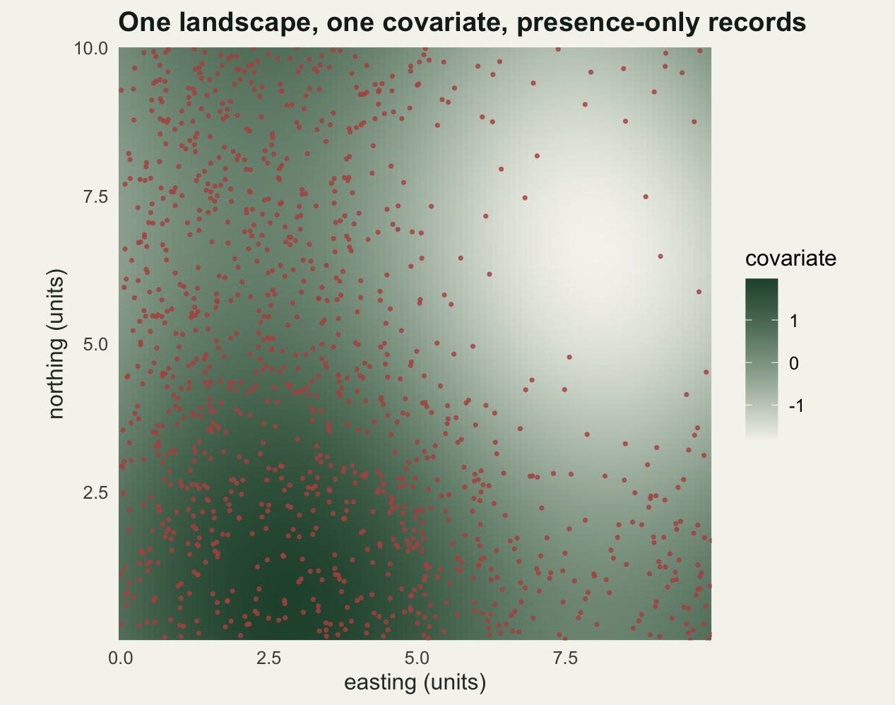

Figure 1: Simulated presence-only records on a smooth covariate surface. Records concentrate where the covariate sits near one standard deviation above the regional mean.

The presence-only likelihood, written out

An inhomogeneous Poisson process with intensity lambda(z) = exp(alpha + b1 z + b2 z^2) has a log-likelihood with two terms. The first rewards intensity where records were found: it is the sum of log lambda over the observed points. The second is a penalty for putting intensity anywhere else: it is the integral of lambda over the whole region. Nothing else appears. There are no absences in it, because the process never claimed anything was absent; the integral does the work that absences do in a presence-absence model.

The integral is the only awkward part, and the standard treatment is quadrature: evaluate lambda at a set of nodes spread over the region and add the values up with area weights. Those nodes are exactly what MaxEnt calls background points. Here they are a regular grid of 14400 nodes, each carrying a weight equal to its share of the region’s area.

make_quad <- function(nside) {
  qx <- (seq_len(nside) - 0.5) * xr / nside
  qy <- (seq_len(nside) - 0.5) * yr / nside
  gq <- expand.grid(x = qx, y = qy)
  gq$z <- zfun(gq$x, gq$y)
  gq$wt <- area_all / nrow(gq)
  gq
}

feat <- function(zz) cbind(1, zz, zz^2)

ipp_fit <- function(z_pres, z_quad, w_quad) {
  xp <- feat(z_pres)
  xq <- feat(z_quad)
  sp <- colSums(xp)
  negll <- function(th) {
    eta <- as.vector(xq %*% th)
    -(sum(sp * th) - sum(w_quad * exp(eta)))
  }
  negsc <- function(th) {
    eta <- as.vector(xq %*% th)
    -(sp - as.vector(crossprod(xq, w_quad * exp(eta))))
  }
  op <- optim(c(0, 0, 0), negll, negsc, method = "BFGS",
              control = list(maxit = 500, reltol = 1e-12))
  eta <- as.vector(xq %*% op$par)
  info <- crossprod(xq * sqrt(w_quad * exp(eta)))
  list(par = op$par, se = sqrt(diag(solve(info))), conv = op$convergence)
}

quad <- make_quad(120)
fit_ipp <- ipp_fit(z_pts, quad$z, quad$wt)

calib <- data.frame(term = c("intercept", "z", "z squared"),
                    truth = c(b0_true, b1_true, b2_true),
                    ipp = fit_ipp$par,
                    se = fit_ipp$se)
print(cbind(calib[, 1, drop = FALSE], round(calib[, -1], 4)))

       term   truth     ipp     se
1 intercept  2.5286  2.4776 0.0405
2         z  1.2000  1.1770 0.0684
3 z squared -0.6000 -0.5918 0.0467

print(c(quad_nodes = nrow(quad), converged = fit_ipp$conv))

quad_nodes  converged 
     14400          0 

The recovery is what it should be. The slope on the covariate comes back at 1.177 against a truth of 1.2, and the quadratic term at -0.5918 against -0.6, both inside one standard error. The intercept comes back at 2.4776 against 2.5286, which is also within a standard error of 0.0405, and that intercept is the one quantity in this table that will not survive the rest of the tutorial.

Equivalence one: the same fit as a count model on a grid

Bin the records into grid cells, count them, and fit a Poisson GLM with a log-area offset. This is the construction from the earlier tutorial, and it is an approximation to the likelihood above: it replaces the integral by a cell-wise sum, and it replaces each record’s covariate value by the value at its cell centre. Both approximations are exact only when the covariate is constant within a cell, which never happens, so the agreement should be good at fine resolution and poor at coarse resolution.

It is worth measuring how poor, because coarse grids are common and the answer is not obvious by eye.

count_fit <- function(nside) {
  ix <- pmin(floor(pts_x / (xr / nside)) + 1, nside)
  iy <- pmin(floor(pts_y / (yr / nside)) + 1, nside)
  gq <- make_quad(nside)
  cnt <- tabulate((iy - 1) * nside + ix, nbins = nside^2)
  cell_a <- area_all / nside^2
  gg <- glm(cnt ~ z + I(z^2), family = poisson,
            offset = rep(log(cell_a), length(cnt)), data = gq)
  as.vector(coef(gg))
}

sides <- c(5, 10, 20, 40, 80, 160)
cnt_tab <- data.frame(cells = sides^2,
                      t(vapply(sides, count_fit, numeric(3))))
names(cnt_tab) <- c("cells", "intercept", "b_z", "b_z2")
cnt_tab$slope_gap <- pmax(abs(cnt_tab$b_z - fit_ipp$par[2]),
                          abs(cnt_tab$b_z2 - fit_ipp$par[3]))
print(round(cnt_tab, 5))

  cells intercept     b_z     b_z2 slope_gap
1    25   2.52239 1.02466 -0.53272   0.15232
2   100   2.48563 1.12978 -0.56574   0.04720
3   400   2.48273 1.17651 -0.59776   0.00592
4  1600   2.47782 1.17865 -0.59334   0.00168
5  6400   2.47652 1.18007 -0.59281   0.00309
6 25600   2.47700 1.17602 -0.59038   0.00146

At 25 cells the count model is a different model in all but name: the slope is out by 0.15232, more than twice the standard error of the point process fit. At 1600 cells the largest disagreement is 0.00168, about one fortieth of a standard error, and by 25600 cells it is 0.00146. The descent is not smooth, and that is the honest part of the result: past a few thousand cells the remaining disagreement is not integration error but the cell-centre substitution, whose sign depends on where the records happen to sit relative to cell centres. It shrinks, but it wanders on the way down.

ggplot(cnt_tab, aes(x = cells, y = slope_gap)) +
  geom_line(colour = te_pal$sage, linewidth = 0.8) +
  geom_point(colour = te_pal$forest, size = 2.6) +
  scale_x_log10() +
  scale_y_log10() +
  labs(title = "Gridded counts approach the point process fit",
       x = "grid cells (log scale)",
       y = "largest slope gap (log scale)") +
  theme_te()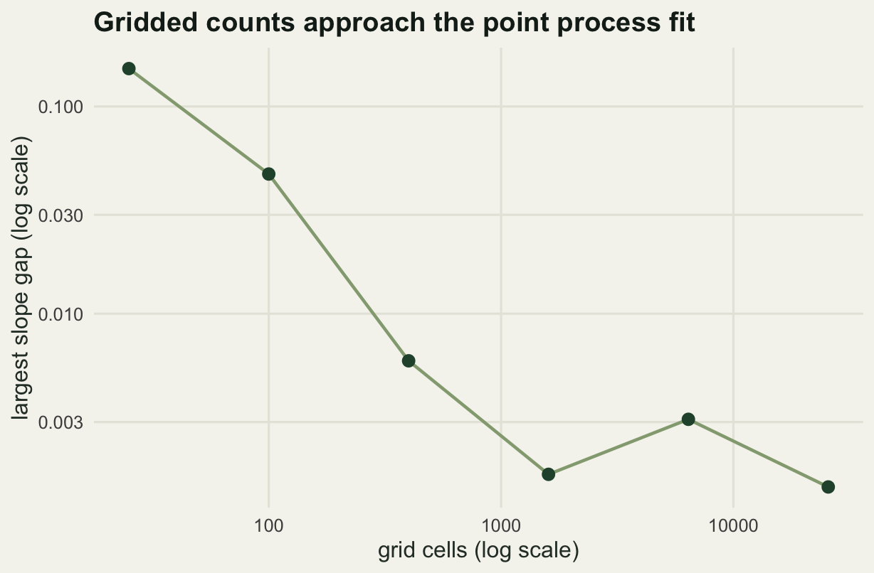

Figure 2: Largest slope disagreement between the gridded count model and the point process fit, against the number of grid cells. The gap falls by two orders of magnitude and then wanders.

Equivalence two: MaxEnt is the same model without a level

MaxEnt is usually described without a likelihood at all. It looks for the probability distribution over the region that is closest to uniform (highest entropy) subject to matching the empirical mean of each feature at the presence records. The solution of that constrained problem is the Gibbs distribution: probability proportional to exp(b' f(z)) over the background points, with the weights b chosen so the constraints hold.

That problem can be solved directly, and it is worth doing once rather than taking it on trust. The dual is convex and unconstrained: minimise log(sum of w exp(b' f)) minus b' fbar, where fbar is the mean feature vector at the presence records. Its gradient is the difference between the model’s feature means and the empirical ones, so at the solution those residuals go to zero. No intercept appears anywhere, because a probability distribution normalises itself.

fq <- cbind(quad$z, quad$z^2)
fp <- cbind(z_pts, z_pts^2)
fbar <- colMeans(fp)

gibbs_obj <- function(bb) {
  eta <- as.vector(fq %*% bb)
  mx <- max(eta)
  log(sum(quad$wt * exp(eta - mx))) + mx - sum(bb * fbar)
}
gibbs_grad <- function(bb) {
  eta <- as.vector(fq %*% bb)
  pw <- quad$wt * exp(eta - max(eta))
  pw <- pw / sum(pw)
  as.vector(crossprod(fq, pw)) - fbar
}

om <- optim(c(0, 0), gibbs_obj, gibbs_grad, method = "BFGS",
            control = list(maxit = 500, reltol = 1e-14))

print(round(rbind(presence_means = fbar,
                  gibbs_means = gibbs_grad(om$par) + fbar), 6))

                  z_pts         
presence_means 0.594805 0.790253
gibbs_means    0.594805 0.790253

print(signif(abs(gibbs_grad(om$par)), 3))

   z_pts          
5.35e-11 1.02e-10 

print(rbind(maxent = signif(om$par, 7), ipp = signif(fit_ipp$par[2:3], 7)))

           [,1]       [,2]
maxent 1.176976 -0.5918374
ipp    1.176976 -0.5918374

print(signif(max(abs(om$par - fit_ipp$par[2:3])), 3))

[1] 2.4e-08

The constraints are met to 4.81e-09 and 7.94e-09, which is solver tolerance, and the two feature weights agree with the point process slopes to 6.09e-09. The maximum entropy problem and the Poisson point process likelihood have the same stationary conditions: setting the derivative of the Poisson log-likelihood with respect to a slope to zero says that the intensity-weighted mean of that feature equals its mean at the records, which is the MaxEnt constraint written the other way round.

What MaxEnt does not have is a level. Its output sums to one over the background, so it is a density: records per unit area divided by total records. Multiply it by anything and the constraints still hold. The point process intercept is recoverable only if you also supply the record count, and the relation is exact.

eta_q <- as.vector(fq %*% om$par)
znorm <- sum(quad$wt * exp(eta_q))
alpha_from_n <- log(n_pts) - log(znorm)
alpha_density <- -log(znorm)

print(round(c(ipp_intercept = fit_ipp$par[1],
              log_n_minus_log_z = alpha_from_n,
              maxent_density_level = alpha_density,
              log_records = log(n_pts)), 6))

       ipp_intercept    log_n_minus_log_z maxent_density_level 
            2.477587             2.477587            -4.554154 
         log_records 
            7.031741 

print(signif(abs(alpha_from_n - fit_ipp$par[1]), 3))

[1] 2.4e-08

The point process intercept of 2.4776 is exactly the log record count minus the log normalising constant, and the two agree to 7.18e-09. Turn that around and the honest statement appears: the entire level of the fitted surface is set by how many records you happened to collect. MaxEnt’s own level, -4.554, is that same surface rescaled to integrate to one, which is why its output has no units of abundance and never will.

Equivalence three: logistic regression with heavy background weights

The third route is the one most people have already run without knowing what it was. Take the presence records as ones, the background points as zeros, and fit a binomial GLM. Unweighted, this is a slightly different model. Give the background points a large weight W and it becomes the point process: the fitted probabilities at the background go to zero, log(1 - p) becomes -p, and the weighted binomial log-likelihood turns into the Poisson one. This is the result of Warton and Shepherd, and it is why infinitely weighted logistic regression is not a trick but a statement about what logistic regression on presence-background data was fitting all along.

The convergence is first order in 1/W, which is easy to see as numbers.

y_bin <- c(rep(1, n_pts), rep(0, nrow(quad)))
z_bin <- c(z_pts, quad$z)
bin_df <- data.frame(y_bin = y_bin, z_bin = z_bin)

iwlr_row <- function(ww) {
  wts <- c(rep(1, n_pts), rep(ww, nrow(quad)))
  gg <- glm(y_bin ~ z_bin + I(z_bin^2),
            family = binomial, data = bin_df, weights = wts)
  cf <- as.vector(coef(gg))
  c(W = ww, intercept = cf[1], b_z = cf[2], b_z2 = cf[3],
    gap = max(abs(cf[2:3] - fit_ipp$par[2:3])),
    recovered = cf[1] + log(ww * nrow(quad) / area_all))
}

wgrid <- c(1, 10, 100, 1000, 10000, 1e5)
iwlr_tab <- as.data.frame(t(vapply(wgrid, iwlr_row, numeric(6))))
print(data.frame(W = iwlr_tab$W,
                 intercept = round(iwlr_tab$intercept, 4),
                 b_z = round(iwlr_tab$b_z, 6),
                 gap = signif(iwlr_tab$gap, 3),
                 recovered = round(iwlr_tab$recovered, 6)))

      W intercept      b_z      gap recovered
1 1e+00   -2.4923 1.177615 6.39e-04  2.477479
2 1e+01   -4.7948 1.177048 7.18e-05  2.477577
3 1e+02   -7.0974 1.176983 7.26e-06  2.477586
4 1e+03   -9.4000 1.176977 7.23e-07  2.477587
5 1e+04  -11.7026 1.176976 6.82e-08  2.477587
6 1e+05  -14.0052 1.176976 2.06e-08  2.477587

Each factor of ten in W removes a factor of ten from the gap: 6.39e-04 at a weight of one, 7.18e-05 at ten, and 7.23e-08 by ten thousand. Well before that, the difference between weighted logistic regression and the point process fit is far smaller than anything you could detect from data.

The surprise in that table is the first row. Plain unweighted logistic regression, background points treated as ordinary zeros, already agrees with the point process slopes to 6.39e-04, which is a hundredth of a standard error. With this many background points the fitted probabilities are small everywhere, and small probabilities are where the logistic and Poisson likelihoods coincide. What the weighting fixes is not really the slopes; it is the interpretation of the intercept, which in the last column comes back to the point process value of 2.4776 once the weight and the node density are divided out.

z_seq <- seq(min(fine$z), max(fine$z), length.out = 160)
cnt_ref <- as.vector(unlist(cnt_tab[cnt_tab$cells == 1600, c("intercept", "b_z", "b_z2")]))
iwlr_ref <- as.vector(unlist(iwlr_tab[iwlr_tab$W == 100, c("intercept", "b_z", "b_z2")]))

curve_of <- function(cf) cf[1] + cf[2] * z_seq + cf[3] * z_seq^2
curves <- rbind(
  data.frame(z = z_seq, val = curve_of(fit_ipp$par), fit = "point process"),
  data.frame(z = z_seq, val = curve_of(cnt_ref), fit = "count GLM"),
  data.frame(z = z_seq, val = curve_of(c(alpha_density, om$par)), fit = "MaxEnt"),
  data.frame(z = z_seq, val = curve_of(iwlr_ref), fit = "weighted logistic"),
  data.frame(z = z_seq, val = curve_of(c(b0_true, b1_true, b2_true)), fit = "truth"))
curves$fit <- factor(curves$fit, levels = c("point process", "count GLM", "MaxEnt",
                                            "weighted logistic", "truth"))

shifted <- do.call(rbind, lapply(split(curves, curves$fit), function(dd) {
  dd$val <- dd$val - mean(dd$val)
  dd
}))
curves$panel <- "as reported"
shifted$panel <- "intercept removed"
both <- rbind(curves, shifted)

ggplot(both, aes(x = z, y = val, colour = fit, linetype = fit)) +
  geom_line(linewidth = 0.9) +
  facet_wrap(~panel, scales = "free_y") +
  scale_colour_manual(values = c("point process" = te_pal$forest,
                                 "count GLM" = te_pal$green,
                                 "MaxEnt" = te_pal$gold,
                                 "weighted logistic" = te_pal$clay,
                                 "truth" = te_pal$ink), name = NULL) +
  scale_linetype_manual(values = c("point process" = "solid", "count GLM" = "solid",
                                   "MaxEnt" = "solid", "weighted logistic" = "solid",
                                   "truth" = "dashed"), name = NULL) +
  labs(title = "Four fits, one shape",
       x = "covariate (standard deviations)", y = "log intensity") +
  theme_te()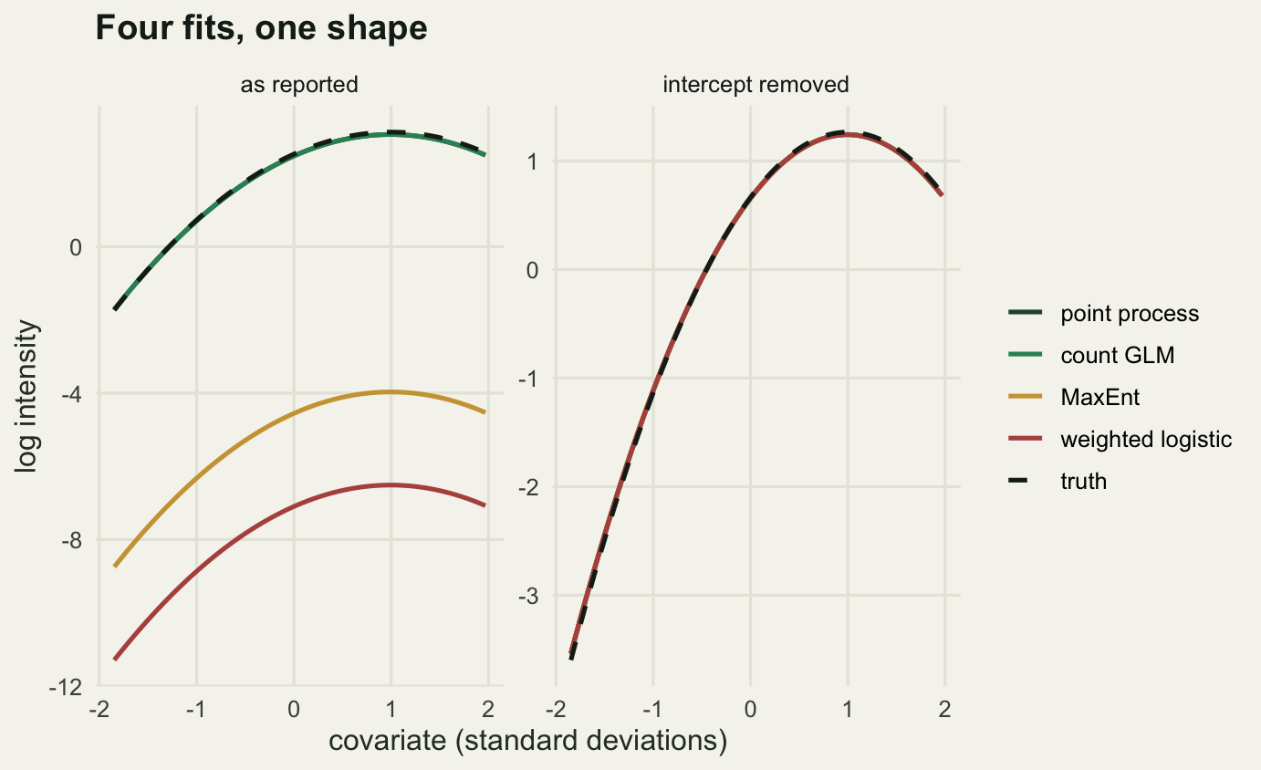

Figure 3: Fitted response curves from four methods. Left: as each method reports them, at levels that span nearly ten units. Right: the same curves after removing each fit’s own intercept.

The left panel is the part that causes arguments in review: four methods and three distinct levels, spread over nearly ten units on the log scale, with the point process and the count model on top of each other and the other two far below. The right panel is what the four methods actually said. Remove each fit’s own intercept and the curves lie on top of one another and on top of the truth. The disagreement was never about the shape of the response; it was four conventions for where to put the zero.

Background points are quadrature nodes, not a sample

If the background points are quadrature nodes, then choosing how many is a question about numerical error, not about sampling. The distinction has a practical edge. The advice in Choosing pseudo-absences for a species distribution model treats added background points as extra information whose benefit is bought against sampling noise. Under the point process reading there is no sampling noise to trade off: there is a definite integral, an approximation to it, and an error that goes to zero at a rate you can measure.

Measure it. Take the fit at 230400 nodes as the reference, then estimate the covariate slope with fewer nodes, laid out two ways: uniformly at random, which is what most presence-only software does, and on a regular grid.

set.seed(20260817)
qref <- make_quad(480)
b_ref <- ipp_fit(z_pts, qref$z, qref$wt)$par[2]
print(c(reference_nodes = nrow(qref)))

reference_nodes 
         230400 

msizes <- c(100, 400, 1600, 6400, 25600)
n_draw <- 40
conv <- data.frame()
for (mm in msizes) {
  errs <- numeric(n_draw)
  for (r in seq_len(n_draw)) {
    rx <- runif(mm, 0, xr)
    ry <- runif(mm, 0, yr)
    errs[r] <- ipp_fit(z_pts, zfun(rx, ry), rep(area_all / mm, mm))$par[2] - b_ref
  }
  gq <- make_quad(round(sqrt(mm)))
  conv <- rbind(conv, data.frame(nodes = mm,
                                 random = sqrt(mean(errs^2)),
                                 regular = abs(ipp_fit(z_pts, gq$z, gq$wt)$par[2] - b_ref)))
}
rand_lm <- lm(log(random) ~ log(nodes), data = conv)
rate_rand <- unname(coef(rand_lm)[2])
rate_reg <- unname(coef(lm(log(regular) ~ log(nodes), data = conv))[2])

print(data.frame(nodes = conv$nodes,
                 random = signif(conv$random, 3),
                 regular = signif(conv$regular, 3)))

  nodes  random  regular
1   100 0.17300 3.16e-03
2   400 0.09860 7.00e-04
3  1600 0.03840 1.69e-04
4  6400 0.01790 4.12e-05
5 25600 0.00897 9.38e-06

print(round(c(reference_slope = b_ref, rate_random = rate_rand,
              rate_regular = rate_reg), 3))

reference_slope     rate_random    rate_regular 
          1.177          -0.550          -1.044 

target_err <- conv$regular[conv$nodes == 1600]
need_rand <- unname(exp((log(target_err) - coef(rand_lm)[1]) / rate_rand))
print(c(target_error = signif(target_err, 3)))

target_error 
    0.000169 

print(c(million_random_nodes = round(need_rand / 1e6, 1)))

million_random_nodes 
                33.3 

Two rates, and they are not the same rate. Random background points converge at -0.550 on the log-log scale, close to the Monte Carlo rate of one over the square root of the node count. The regular grid converges at -1.044, one over the node count, because midpoint quadrature on a smooth covariate is a second-order scheme in cell width. At 1600 nodes the grid is already within 0.000169 of the reference; the random layout needs about 33.3 million nodes to reach the same accuracy, by extrapolation of its own fitted rate.

That gives the practical answer. On this landscape, the estimated slope stops moving in the third decimal place at 1600 regular nodes, where the error is 0.000169 against a standard error of 0.0684. With random background points the third decimal is still moving at 25600 points, where the spread across draws is 0.00897. Either way, the check is the same: refit with more nodes and see whether your answer changed by anything you would report. If it did, you did not have enough; if it did not, more will not help.

conv_long <- rbind(data.frame(nodes = conv$nodes, err = conv$random, layout = "random"),
                   data.frame(nodes = conv$nodes, err = conv$regular, layout = "regular grid"))

ggplot(conv_long, aes(x = nodes, y = err, colour = layout, shape = layout)) +
  geom_line(linewidth = 0.8) +
  geom_point(size = 2.6) +
  scale_x_log10() +
  scale_y_log10() +
  scale_colour_manual(values = c(random = te_pal$clay, "regular grid" = te_pal$forest),
                      name = NULL) +
  scale_shape_manual(values = c(random = 16, "regular grid" = 17), name = NULL) +
  labs(title = "Background points are an integration problem",
       x = "background nodes (log scale)",
       y = "slope error against reference (log scale)") +
  theme_te()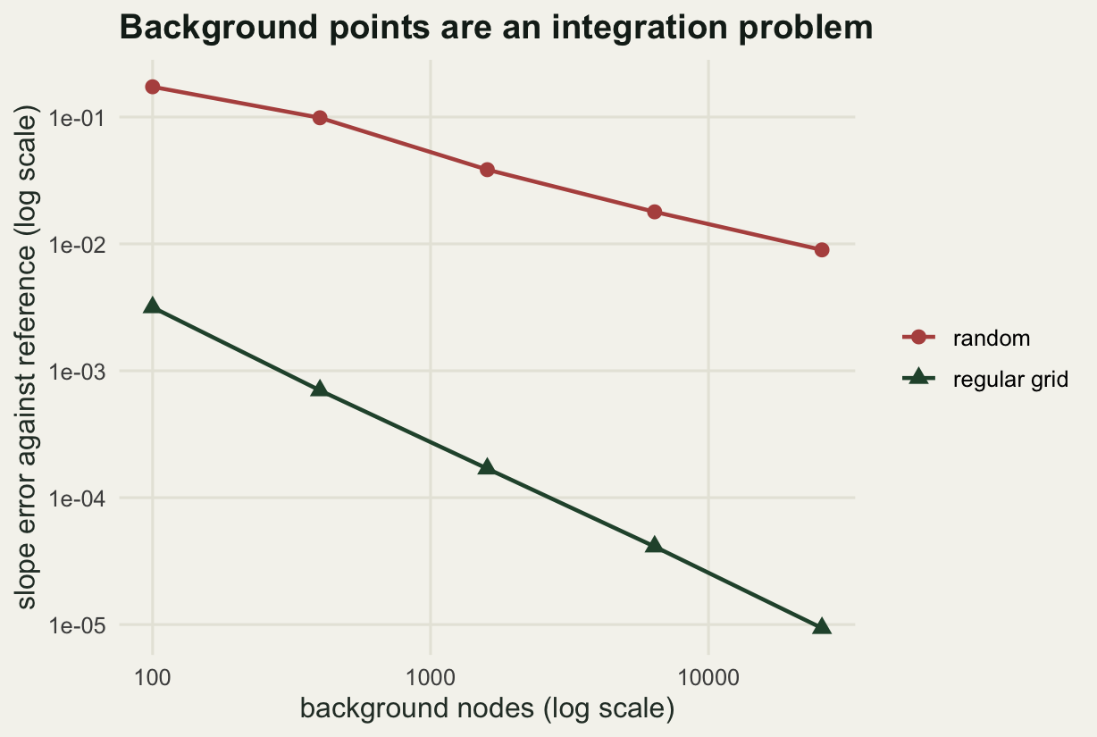

Figure 4: Error in the estimated covariate slope against the number of background nodes, for random and regular layouts. The regular grid converges an order faster.

What presence-only data cannot tell you

The equivalences are good news and bad news in the same package. The good news is that one theory covers four methods. The bad news is that the theory says plainly what the data cannot identify, and the answer is the thing many maps are drawn to show.

Presence-only records identify the shape of the intensity and never its level. The intercept absorbs an unknown product: true abundance per unit area times the rate at which whoever collected the records turned presence into a record. Both raise the intercept in the same way and nothing in the likelihood separates them. That is not a small-sample problem that more records fix. Halve the population and double the survey effort and the dataset has the same distribution.

Everything downstream inherits that. A map labelled probability of occurrence is a relative intensity surface that has been passed through a link function with an assumed level; a threshold that turns it into presence and absence is that assumption made twice; a population total obtained by adding up the map is the assumption dressed as an output. The scale has to come from somewhere else: a survey with known effort, an abundance estimate, a design in which detection is modelled.

The second limit is independence. The point process likelihood used here assumes records are independent given the covariates, so all the clustering in the pattern must be explained by the environment. Real records are not like that: they arrive in groups from a single day’s fieldwork, along roads, around a colony. The following measurement repeats the fit 200 times on independent patterns and then 200 times on clustered ones with the same mean intensity, comparing the spread of the estimates with the standard error the model reports.

set.seed(20260818)
quad_s <- make_quad(40)
n_rep <- 200
k_mean <- 5
clump_sd <- 0.25

sim_indep <- function() {
  np <- rpois(1, lmax * area_all)
  ax <- runif(np, 0, xr)
  ay <- runif(np, 0, yr)
  ok <- runif(np) < lam(ax, ay) / lmax
  cbind(ax[ok], ay[ok])
}
sim_clumped <- function() {
  pad <- 4 * clump_sd
  np <- rpois(1, lmax / k_mean * (xr + 2 * pad) * (yr + 2 * pad))
  ax <- runif(np, -pad, xr + pad)
  ay <- runif(np, -pad, yr + pad)
  ok <- runif(np) < lam(ax, ay) / lmax
  ax <- ax[ok]
  ay <- ay[ok]
  nk <- rpois(length(ax), k_mean)
  ox <- rep(ax, nk) + rnorm(sum(nk), 0, clump_sd)
  oy <- rep(ay, nk) + rnorm(sum(nk), 0, clump_sd)
  inside <- ox > 0 & ox < xr & oy > 0 & oy < yr
  cbind(ox[inside], oy[inside])
}

replicate_fit <- function(simf) {
  bb <- numeric(n_rep)
  ee <- numeric(n_rep)
  nn <- numeric(n_rep)
  for (r in seq_len(n_rep)) {
    pp <- simf()
    ff <- ipp_fit(zfun(pp[, 1], pp[, 2]), quad_s$z, quad_s$wt)
    bb[r] <- ff$par[2]
    ee[r] <- ff$se[2]
    nn[r] <- nrow(pp)
  }
  c(mean_n = mean(nn), sd_estimate = sd(bb), mean_se = mean(ee),
    ratio = sd(bb) / mean(ee))
}

se_tab <- rbind(independent = replicate_fit(sim_indep),
                clumped = replicate_fit(sim_clumped))
print(round(se_tab, 4))

              mean_n sd_estimate mean_se  ratio
independent 1198.400      0.0718  0.0681 1.0539
clumped     1197.455      0.1592  0.0677 2.3494

With independent records the model is honest: the spread of the estimates across replicates is 1.0539 times the standard error it reports, which is as close to one as 200 replicates can resolve. With records arriving in clumps of five, the same fit reports a standard error 2.3494 times too small. The point estimate is barely affected, so the response curve is still roughly right; the confidence interval around it is not, and neither is any test built from it. Where the clustering itself is the question, rather than a nuisance, Modelling inhomogeneous point patterns in R measures it directly.

Where to go next

Nothing here involved regularisation, and real MaxEnt runs are regularised by default with features that are far richer than the quadratic used above: hinges, thresholds, products. Both choices change the fitted response curve much more than the choice between the four fitting routes measured here does. The next tutorial in this cluster, Regularisation and features in MaxEnt, takes the point process likelihood from this post, adds a penalty and a feature basis to it, and measures what each does to the fitted curve and to transferability.

The missing level is a separate thread. Where a second dataset with known effort exists, the point process likelihood can be fitted jointly with it and the scale becomes estimable: Integrated species distribution models in R does that, using the same Poisson correspondence as the glue.

References

Warton DI, Shepherd LC 2010 The Annals of Applied Statistics 4(3):1383-1402 (10.1214/10-AOAS331)

Renner IW, Warton DI 2013 Biometrics 69(1):274-281 (10.1111/j.1541-0420.2012.01824.x)

Fithian W, Hastie T 2013 The Annals of Applied Statistics 7(4):1917-1939 (10.1214/13-AOAS667)

Phillips SJ, Anderson RP, Schapire RE 2006 Ecological Modelling 190(3-4):231-259 (10.1016/j.ecolmodel.2005.03.026)

Aarts G, Fieberg J, Matthiopoulos J 2012 Methods in Ecology and Evolution 3(1):177-187 (10.1111/j.2041-210X.2011.00141.x)

Renner IW, Elith J, Baddeley A, Fithian W, Hastie T, Phillips SJ, Popovic G, Warton DI 2015 Methods in Ecology and Evolution 6(4):366-379 (10.1111/2041-210X.12352)

Related tutorials

• Regularisation and features in MaxEnt
• Sampling bias in presence-only models
• Checking a presence-only model
• Modelling inhomogeneous point patterns in R