library(ggplot2)

te_pal <- list(forest = "#275139", green = "#2f8f63", sage = "#93a87f",
               clay = "#b5534e", gold = "#cda23f", line = "#dad9ca",
               ink = "#16241d", paper = "#f5f4ee")

theme_te <- function() {
  theme_minimal(base_size = 12) +
    theme(panel.grid.minor = element_blank(),
          panel.grid.major = element_line(colour = "#e7e6dc"),
          plot.background = element_rect(fill = "#f5f4ee", colour = NA),
          panel.background = element_rect(fill = "#f5f4ee", colour = NA),
          plot.title = element_text(face = "bold", colour = te_pal$ink),
          axis.title = element_text(colour = "#2c3a31"))
}Regularisation and features in MaxEnt
R
MaxEnt
species distributions
regularisation
presence-only
ecology tutorial
ggplot2
How the MaxEnt feature classes and the regularisation multiplier work, built by hand in R, and what each setting does to a fitted species response curve.
Two settings in MaxEnt get changed by almost everyone and explained by almost nobody: the tick boxes that turn feature classes on and off, and the box holding the regularisation multiplier. The software offers them as preferences, the way a printer dialogue offers paper sizes. They are not preferences. Between them they decide how many columns the model is allowed to invent from your environmental layers, and how hard the fitting is pushed to set most of those columns to zero.
The sibling tutorial MaxEnt as a Poisson point process establishes what the fitting actually is: a penalised inhomogeneous Poisson point process, with the background points acting as quadrature nodes for the integral of the intensity. I take that as given here. The penalty itself is an L1 penalty, the same soft-thresholding machinery implemented in The lasso and variable selection, so I will not re-derive the optimiser from first principles. What is new here is that the penalty acts on features the software generated for you, not on variables you chose, and that the thing being shrunk is the shape of a species response curve.
Everything below runs on a simulated presence-only dataset where the true response curve is known, so that every claim can be checked against something. All likelihoods are reported as nats per record, measured against a uniform map: zero means the model is worth no more than a blank raster, and the highest value any model could reach on this simulation is printed below. The measurements are: how fast the feature count grows, what an unpenalised fit does to a response curve, where the held-out optimum on the path sits and how asymmetric it is, whether the sample-size rule the software encodes matches the one I can measure, which feature class wins when each is tuned fairly, and how much of a tuned held-out score is selection bias.
Two covariates, 125 columns
The study area is a square grid of cells. Two environmental covariates run across it: env1, rank-transformed so that the grid covers its range evenly, and env2, a smoother field left as it is. The true log-intensity is a sharp peak in env1 with a shoulder on its upper side, plus a weak linear term in env2. Records are drawn from the cells with probability proportional to intensity, which is the point process conditioned on the number of records.
set.seed(20260816)
side <- 45
gx <- rep(seq(0, 1, length.out = side), times = side)
gy <- rep(seq(0, 1, length.out = side), each = side)
ncell <- side * side

smooth_field <- function(px, py, npeak, wid) {
  cx <- runif(npeak); cy <- runif(npeak); amp <- rnorm(npeak)
  z <- numeric(length(px))
  for (k in seq_len(npeak)) z <- z + amp[k] * exp(-((px - cx[k])^2 + (py - cy[k])^2) / wid)
  z
}
env1 <- (rank(smooth_field(gx, gy, 14, 0.03)) - 0.5) / ncell
raw2 <- smooth_field(gx, gy, 10, 0.04)
env2 <- (raw2 - min(raw2)) / (max(raw2) - min(raw2))

true_resp <- function(u) 4.5 * exp(-0.5 * ((u - 0.45) / 0.09)^2) +
                         2.0 * exp(-0.5 * ((u - 0.76) / 0.15)^2)
eta_true <- true_resp(env1) + 0.9 * env2
pcell <- exp(eta_true) / sum(exp(eta_true))
cat("cells:", ncell, " correlation env1 env2:", round(cor(env1, env2), 3), "\n")
cells: 2025 correlation env1 env2: 0.162 cat("intensity ratio, hottest cell to average cell:", round(max(pcell) * ncell, 2), "\n")intensity ratio, hottest cell to average cell: 9.52 cat("information in the truth (nats per record):",
round(sum(pcell * log(pcell * ncell)), 3), "\n")information in the truth (nats per record): 0.961 draw_records <- function(nrec) sample.int(ncell, nrec, replace = TRUE, prob = pcell)
set.seed(4001)
eval_rec <- draw_records(4000)
cat("evaluation records:", length(eval_rec),
" ceiling reachable on them:", round(mean(log(pcell[eval_rec] * ncell)), 4), "\n")evaluation records: 4000 ceiling reachable on them: 0.9381 The hottest cell holds 9.52 times the average intensity, and a model that knew the truth exactly would score 0.9381 nats per record on the evaluation draw. That is the number every fit below is chasing.
Now the features. MaxEnt does not fit your covariates; it fits transformations of them, rescaled to the unit interval over the background. Linear features are the covariates themselves. Quadratic features are their squares. Product features are pairwise products. A threshold feature is a step: one on the far side of a knot, zero on the near side. A hinge feature is a ramp that is flat on one side of a knot and rises linearly on the other, and each knot yields two of them, one facing each way. The knot grid is what makes the count explode.
raw_features <- function(classes, knots, u1, u2) {
  blocks <- list()
  if ("linear" %in% classes)    blocks$lin <- cbind(u1, u2)
  if ("quadratic" %in% classes) blocks$qua <- cbind(u1^2, u2^2)
  if ("product" %in% classes)   blocks$pro <- cbind(u1 * u2)
  if ("threshold" %in% classes)
    blocks$thr <- cbind(outer(u1, knots, function(a, k) as.numeric(a > k)),
                        outer(u2, knots, function(a, k) as.numeric(a > k)))
  if ("hinge" %in% classes)
    blocks$hin <- cbind(outer(u1, knots, function(a, k) pmax(0, a - k)),
                        outer(u1, knots, function(a, k) pmax(0, k - a)),
                        outer(u2, knots, function(a, k) pmax(0, a - k)),
                        outer(u2, knots, function(a, k) pmax(0, k - a)))
  do.call(cbind, blocks)
}

make_spec <- function(classes, nknot, one_var = FALSE) {
  kn <- if (nknot > 0) seq(0, 1, length.out = nknot + 2)[-c(1, nknot + 2)] else numeric(0)
  second <- if (one_var) rep(0, ncell) else env2
  fmat <- raw_features(classes, kn, env1, second)
  flo <- apply(fmat, 2, min); fhi <- apply(fmat, 2, max)
  keep <- fhi > flo
  sp <- list(classes = classes, knots = kn, lo = flo[keep], hi = fhi[keep],
             keep = keep, one_var = one_var)
  sp$bg <- sweep(sweep(fmat[, keep, drop = FALSE], 2, sp$lo, "-"), 2, sp$hi - sp$lo, "/")
  sp$pen <- apply(sp$bg, 2, sd)
  sp
}
spec_apply <- function(sp, u1, u2) {
  fmat <- raw_features(sp$classes, sp$knots, u1,
                       if (sp$one_var) rep(0, length(u1)) else u2)[, sp$keep, drop = FALSE]
  sweep(sweep(fmat, 2, sp$lo, "-"), 2, sp$hi - sp$lo, "/")
}

count_features <- function(nknot, nvar) {
  data.frame(knots = nknot,
             linear = nvar, quadratic = nvar, product = nvar * (nvar - 1) / 2,
             threshold = nvar * nknot, hinge = 2 * nvar * nknot,
             total = 2 * nvar + nvar * (nvar - 1) / 2 + 3 * nvar * nknot)
}
print(do.call(rbind, lapply(c(2, 5, 10, 20, 40), count_features, nvar = 2)),
      row.names = FALSE)
knots linear quadratic product threshold hinge total
2 2 2 1 4 8 17
5 2 2 1 10 20 35
10 2 2 1 20 40 65
20 2 2 1 40 80 125
40 2 2 1 80 160 245spec_all <- make_spec(c("linear", "quadratic", "product", "threshold", "hinge"), 20)
cat("features in the full 20-knot basis, two covariates:", ncol(spec_all$bg), "\n")features in the full 20-knot basis, two covariates: 125 Two measured variables and a 20-knot grid give 125 columns, of which 120 are threshold and hinge features. Push the knot grid to 40 and it is 245. The real software places knots at observed covariate values, so the count grows with your sample rather than with a setting, but the arithmetic is the same: the model dimension is set by the feature machinery, not by the number of things you measured in the field. This is why regularisation in MaxEnt is not a refinement. Without it there is nothing at all standing between 150 records and 125 free parameters.
No penalty at all
The objective is the MaxEnt objective written as a density over the background cells: the mean of the linear predictor over the presence records, minus the log of the mean of its exponential over the background, minus the penalty. Written that way there is no intercept, because the normalising term absorbs it, and the presence records enter only through their feature means. The gradient is the difference between the empirical feature mean and the feature mean under the fitted density, which is the moment-matching statement MaxEnt is usually introduced with. I maximise it by accelerated proximal gradient: a gradient step, then soft-thresholding, with a backtracking line search on the step length.
soft_thr <- function(z, thr) sign(z) * pmax(abs(z) - thr, 0)

fit_maxent <- function(sp, fbar, lam, b0 = NULL, n_iter = 200, tol = 1e-11) {
  fbg <- sp$bg
  bprev <- if (is.null(b0)) numeric(ncol(fbg)) else b0
  gain <- function(bb) {
    ee <- fbg %*% bb; top <- max(ee)
    sum(fbar * bb) - (top + log(mean(exp(ee - top))))
  }
  gradient <- function(bb) {
    ee <- fbg %*% bb; wts <- exp(ee - max(ee)); wts <- wts / sum(wts)
    as.numeric(fbar - crossprod(fbg, wts))
  }
  stp <- 1; ycur <- bprev; mom <- 1
  for (it in seq_len(n_iter)) {
    gy <- gain(ycur); dy <- gradient(ycur)
    repeat {
      bnew <- soft_thr(ycur + stp * dy, stp * lam)
      dl <- bnew - ycur
      if (gain(bnew) >= gy + sum(dy * dl) - sum(dl^2) / (2 * stp) - 1e-14) break
      stp <- stp / 2
      if (stp < 1e-12) break
    }
    mnew <- (1 + sqrt(1 + 4 * mom^2)) / 2
    ycur <- bnew + ((mom - 1) / mnew) * (bnew - bprev)
    stop_now <- sum(abs(bnew - bprev)) < tol * (1 + sum(abs(bnew)))
    bprev <- bnew; mom <- mnew; stp <- stp * 1.1
    if (stop_now) break
  }
  list(bhat = bprev, grad = gradient(bprev), gain = gain(bprev), iters = it)
}

log_density <- function(sp, bhat) {
  ee <- as.numeric(sp$bg %*% bhat)
  ee - (max(ee) + log(mean(exp(ee - max(ee)))))
}
ugrid <- seq(0, 1, length.out = 101)
env2_mid <- median(env2)
resp_curve <- function(sp, bhat) {
  ee <- as.numeric(spec_apply(sp, ugrid, rep(env2_mid, length(ugrid))) %*% bhat)
  ee - mean(ee)
}
true_curve <- true_resp(ugrid) - mean(true_resp(ugrid))
roughness <- function(cv) sum(diff(cv, differences = 2)^2)
shape_err <- function(cv) sqrt(mean((cv - true_curve)^2))
cat("shape error of a flat response curve:", round(shape_err(rep(0, 101)), 3), "\n")
shape error of a flat response curve: 1.424 path_fit <- function(sp, idx, mults, n_iter = 200) {
fbar <- colMeans(sp$bg[idx, , drop = FALSE])
unit <- sp$pen / sqrt(length(idx))
b0 <- NULL; out <- vector("list", length(mults))
for (k in rev(seq_along(mults))) {
ft <- fit_maxent(sp, fbar, mults[k] * unit, b0 = b0, n_iter = n_iter)
b0 <- ft$bhat; out[[k]] <- ft
}
out
}Set the penalty to zero and run the solver on 150 records with all 125 features. The interesting part is not the fit but what happens as the solver keeps going.
set.seed(1207)
rec <- draw_records(150)
cat("training records:", length(rec), " distinct cells:", length(unique(rec)), "\n")
training records: 150 distinct cells: 133 fbar_all <- colMeans(spec_all$bg[rec, ])
zero_pen <- rep(0, ncol(spec_all$bg))
budget <- c(250, 750, 1500)
warm <- NULL; over <- NULL; curves_over <- NULL
for (b in seq_along(budget)) {
extra <- if (b == 1) budget[1] else budget[b] - budget[b - 1]
ft <- fit_maxent(spec_all, fbar_all, zero_pen, b0 = warm, n_iter = extra, tol = 0)
warm <- ft$bhat
ld <- log_density(spec_all, warm)
over <- rbind(over, data.frame(steps = budget[b], train = mean(ld[rec]),
held_out = mean(ld[eval_rec]),
biggest = max(abs(warm))))
curves_over <- rbind(curves_over,
data.frame(u = ugrid, fit = resp_curve(spec_all, warm), steps = budget[b]))
}
print(round(over, 4), row.names = FALSE) steps train held_out biggest
250 0.9948 0.6805 7.6923
750 1.0318 0.5826 18.0839
1500 1.0414 0.5276 22.2264From 250 steps to 1500 steps the training likelihood improves from 0.9948 to 1.0414, a gain of about 0.047 nats, while the held-out likelihood falls from 0.6805 to 0.5276, a loss of 0.153. The largest coefficient grows from 7.6923 to 22.2264 and is still growing. There is no finite unpenalised maximum here to converge to: the solver walks towards the edge of the parameter space, buying an ever smaller gain in training likelihood with a response curve that plunges by six log units in the gaps between records. The figure shows where it goes.
show_knots <- c(0.25, 0.5, 0.75)
feat_dat <- do.call(rbind, lapply(show_knots, function(kk) rbind(
  data.frame(u = ugrid, val = pmax(0, ugrid - kk), series = paste0("forward ", kk)),
  data.frame(u = ugrid, val = pmax(0, kk - ugrid), series = paste0("reverse ", kk)))))
feat_dat$panel <- "hinge features at knots 0.25, 0.5 and 0.75"
fit_dat <- rbind(
  data.frame(u = ugrid, val = true_curve, series = "truth"),
  data.frame(u = curves_over$u, val = curves_over$fit,
             series = paste(curves_over$steps, "steps")))
fit_dat <- fit_dat[fit_dat$series != "750 steps", ]
fit_dat$panel <- "unpenalised fit, 125 features, 150 records"
p_basis <- ggplot(fit_dat, aes(u, val, colour = series)) +
  geom_line(data = feat_dat, aes(group = series), colour = te_pal$sage, linewidth = 0.7) +
  geom_rug(data = data.frame(u = env1[rec], val = 0, series = "truth",
                             panel = "unpenalised fit, 125 features, 150 records"),
           sides = "b", colour = te_pal$ink, alpha = 0.3, show.legend = FALSE) +
  geom_line(linewidth = 0.8) +
  facet_wrap(~panel, ncol = 1, scales = "free_y") +
  scale_colour_manual(values = c("truth" = te_pal$forest, "250 steps" = te_pal$gold,
                                 "1500 steps" = te_pal$clay)) +
  labs(x = "environmental covariate, rescaled to the unit interval",
       y = "feature value or centred log-intensity",
       colour = NULL, title = "A basis with 125 columns and nothing holding it back") +
  theme_te()
p_basis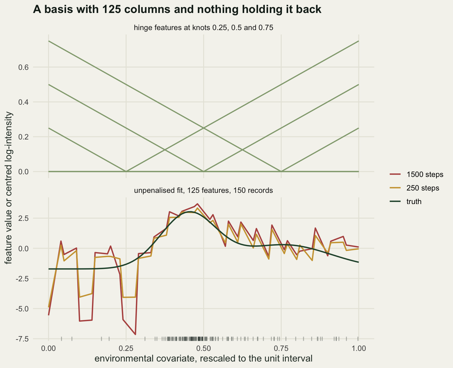
The penalty, and how to check it
MaxEnt does not use one penalty weight for all features. Each feature gets its own regularisation value, roughly proportional to the spread of that feature over the background and shrinking as the number of presence records grows. I use lam_j = mult * sd_j / sqrt(m), with mult the multiplier the software exposes. The scale factor matters: a threshold feature that is one almost everywhere has a tiny standard deviation and buys a nearly free coefficient, while a feature that splits the background in half is penalised hardest.
The optimality condition is the one every L1 problem has. At the solution, an active feature satisfies gradient_j = lam_j * sign(beta_j), and a feature left at zero satisfies |gradient_j| <= lam_j. Since the gradient here is the empirical feature mean minus the fitted feature mean, that condition says something concrete: the fit must reproduce the empirical mean of every retained feature exactly to within its own regularisation value, and may miss it by no more than that for the features it drops. Regularisation in MaxEnt is a tolerance on moment matching, and the multiplier sets how wide the tolerance is.
unit_pen <- spec_all$pen / sqrt(length(rec))
cat("per-feature penalty at multiplier 1: min", signif(min(unit_pen), 3),
    " median", signif(median(unit_pen), 3), " max", signif(max(unit_pen), 3), "\n")
per-feature penalty at multiplier 1: min 0.00507 median 0.0234 max 0.0408 one_fit <- fit_maxent(spec_all, fbar_all, 0.5 * unit_pen, n_iter = 900)
active <- one_fit$bhat != 0
lam_here <- 0.5 * unit_pen
viol_active <- if (any(active))
max(abs(one_fit$grad[active] - lam_here[active] * sign(one_fit$bhat[active]))) else 0
viol_zero <- max(0, max(abs(one_fit$grad[!active]) - lam_here[!active]))
cat("non-zero features:", sum(active), "\n")non-zero features: 17 cat("max subgradient violation, active set:", signif(viol_active, 3), "\n")max subgradient violation, active set: 6.57e-07 cat("max subgradient violation, zero set:", signif(viol_zero, 3), "\n")max subgradient violation, zero set: 0 cat("largest gap between empirical and fitted feature mean:",
round(max(abs(one_fit$grad)), 4), "\n")largest gap between empirical and fitted feature mean: 0.0204 At a multiplier of 0.5 the fit keeps 17 of the 125 features, satisfies the active-set condition to 6.57e-07 and violates the zero-set condition nowhere. The largest distance between an empirical and a fitted feature mean is 0.0204, on features scaled to the unit interval.
The zero-penalty case needs a basis where the maximum likelihood fit is a finite, unique point, which the 125-column basis is not. On linear and quadratic features only, the same fit can be had from a Poisson regression on the cell counts, which is a standard equivalence and an entirely separate piece of code.
spec_lq <- make_spec(c("linear", "quadratic"), 0)
fbar_lq <- colMeans(spec_lq$bg[rec, ])
mine <- fit_maxent(spec_lq, fbar_lq, rep(0, ncol(spec_lq$bg)), n_iter = 4000, tol = 1e-13)
counts <- tabulate(rec, nbins = ncell)
glm_fit <- glm(counts ~ spec_lq$bg, family = poisson)
cat("own solver: ", paste(round(mine$bhat, 4), collapse = " "), "\n")
own solver: 20.8318 2.0502 -20.0612 -2.093 cat("Poisson glm:", paste(round(coef(glm_fit)[-1], 4), collapse = " "), "\n")Poisson glm: 20.8318 2.0502 -20.0612 -2.093 cat("largest coefficient difference:", signif(max(abs(mine$bhat - coef(glm_fit)[-1])), 3), "\n")largest coefficient difference: 4.82e-11 Agreement to 4.82e-11. The solver is doing what it claims.
The path
Sweep the multiplier from 0.01 to about 8 and record five things at each value: how many features survive, the training likelihood, the held-out likelihood on the 4000 evaluation records, a roughness measure of the fitted response curve, and the shape error of that curve against the truth. Roughness here is the sum of squared second differences on a fixed 101-point grid.
mults <- 10^seq(-2, 0.9, length.out = 13)
fits <- path_fit(spec_all, rec, mults, n_iter = 220)
path_tab <- do.call(rbind, lapply(seq_along(mults), function(k) {
  ld <- log_density(spec_all, fits[[k]]$bhat)
  cv <- resp_curve(spec_all, fits[[k]]$bhat)
  data.frame(multiplier = mults[k], nonzero = sum(fits[[k]]$bhat != 0),
             train = mean(ld[rec]), held_out = mean(ld[eval_rec]),
             rough = roughness(cv), shape = shape_err(cv))
}))
print(format(round(path_tab, 3), nsmall = 3), row.names = FALSE)
multiplier nonzero train held_out rough shape
0.010 91.000 1.003 0.697 102.631 0.935
0.017 68.000 0.991 0.727 77.960 0.819
0.030 61.000 0.970 0.762 51.289 0.691
0.053 47.000 0.941 0.795 32.924 0.582
0.093 41.000 0.900 0.829 18.908 0.499
0.162 29.000 0.856 0.847 13.827 0.454
0.282 23.000 0.835 0.853 12.555 0.453
0.492 18.000 0.811 0.854 11.857 0.473
0.858 15.000 0.783 0.843 10.259 0.543
1.496 8.000 0.719 0.798 8.316 0.666
2.610 6.000 0.630 0.695 5.633 0.838
4.553 6.000 0.396 0.427 1.793 1.100
7.943 0.000 0.000 0.000 0.000 1.424best_k <- which.max(path_tab$held_out)
cat("best multiplier:", round(mults[best_k], 3),
" held-out:", round(path_tab$held_out[best_k], 4),
" non-zero:", path_tab$nonzero[best_k], "\n")best multiplier: 0.492 held-out: 0.8541 non-zero: 18 lgm <- log10(mults)
approx_te <- function(target) approx(lgm, path_tab$held_out, log10(target))$y
loss_low <- path_tab$held_out[best_k] - approx_te(mults[best_k] / 4)
loss_high <- path_tab$held_out[best_k] - approx_te(mults[best_k] * 4)
cat("held-out loss at a quarter of the best multiplier:", round(loss_low, 4), "\n")held-out loss at a quarter of the best multiplier: 0.016 cat("held-out loss at four times the best multiplier:", round(loss_high, 4), "\n")held-out loss at four times the best multiplier: 0.1066 cat("ratio:", round(loss_high / loss_low, 2), "\n")ratio: 6.66 flat <- mults[path_tab$held_out > path_tab$held_out[best_k] - 0.01]
cat("multipliers within 0.01 nats of the best:", round(min(flat), 3), "to", round(max(flat), 3),
" a factor of", round(max(flat) / min(flat), 1), "\n")multipliers within 0.01 nats of the best: 0.162 to 0.492 a factor of 3 The training likelihood is monotone in the wrong direction, as it must be: it is highest at the smallest multiplier and falls all the way down the path. The held-out likelihood has an interior maximum at a multiplier of 0.492, worth 0.8541 nats against a ceiling of 0.9381, with 18 features left of 125.
The asymmetry is the part worth taking away. Going four times below the optimum costs 0.016 nats. Going four times above costs 0.1066, which is 6.66 times as much. In this simulation over-regularising is the more expensive mistake, which is the opposite of the received advice that MaxEnt’s defaults produce overfitted models. The reason is visible in the path table: too little penalty leaves a curve that is right where the records are and wrong in the gaps, and the gaps hold few evaluation records; too much penalty flattens the peak itself, which is where nearly all the evaluation records are. Anything from a multiplier of 0.162 to 0.492, a factor of 3, is within 0.01 nats of the best value, so the optimum is a plateau rather than a point.
plong <- rbind(
  data.frame(multiplier = path_tab$multiplier, val = path_tab$held_out,
             series = "held out", panel = "log-likelihood per record"),
  data.frame(multiplier = path_tab$multiplier, val = path_tab$train,
             series = "training", panel = "log-likelihood per record"),
  data.frame(multiplier = path_tab$multiplier, val = path_tab$nonzero,
             series = "structure", panel = "non-zero features"),
  data.frame(multiplier = path_tab$multiplier, val = path_tab$rough,
             series = "structure", panel = "response curve roughness"))
p_path <- ggplot(plong, aes(multiplier, val, colour = series)) +
  geom_vline(xintercept = mults[best_k], linetype = "dashed",
             colour = te_pal$ink, alpha = 0.5) +
  geom_line(linewidth = 0.8) + geom_point(size = 1.6) +
  facet_wrap(~panel, ncol = 1, scales = "free_y") +
  scale_x_log10() +
  scale_colour_manual(values = c("held out" = te_pal$clay, "training" = te_pal$green,
                                 "structure" = te_pal$ink),
                      breaks = c("held out", "training")) +
  labs(x = "regularisation multiplier, log scale",
       y = NULL, colour = NULL, title = "What the multiplier buys and what it costs") +
  theme_te()
p_path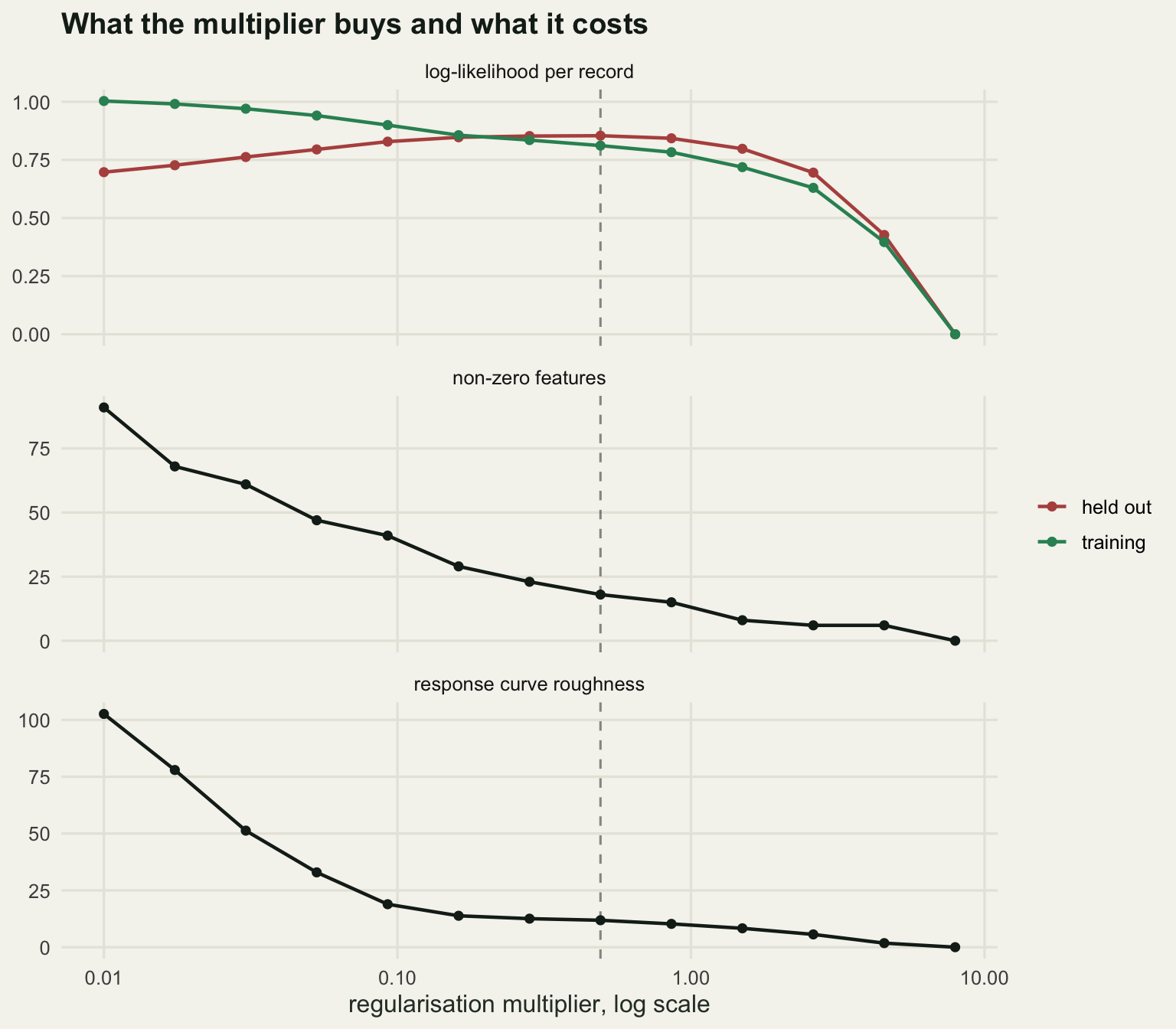
Three fits from that path, drawn against the truth, show what the numbers mean for a response curve.
pick <- c(3, best_k, 11)
pick_lab <- paste("multiplier", format(round(mults[pick], 3), nsmall = 3))
curve_dat <- do.call(rbind, lapply(seq_along(pick), function(j)
  data.frame(u = ugrid, val = resp_curve(spec_all, fits[[pick[j]]]$bhat),
             series = pick_lab[j])))
curve_dat <- rbind(curve_dat, data.frame(u = ugrid, val = true_curve, series = "truth"))
p_curves <- ggplot(curve_dat, aes(u, val, colour = series, linetype = series)) +
  geom_rug(data = data.frame(u = env1[rec], val = 0, series = "truth"),
           sides = "b", colour = te_pal$ink, alpha = 0.3, show.legend = FALSE) +
  geom_line(linewidth = 0.9) +
  scale_colour_manual(values = setNames(c(te_pal$gold, te_pal$green, te_pal$clay,
                                          te_pal$forest), c(pick_lab, "truth"))) +
  scale_linetype_manual(values = setNames(c("solid", "solid", "solid", "22"),
                                          c(pick_lab, "truth"))) +
  labs(x = "environmental covariate", y = "centred log-intensity",
       colour = NULL, linetype = NULL, title = "Three multipliers, one truth") +
  theme_te()
p_curves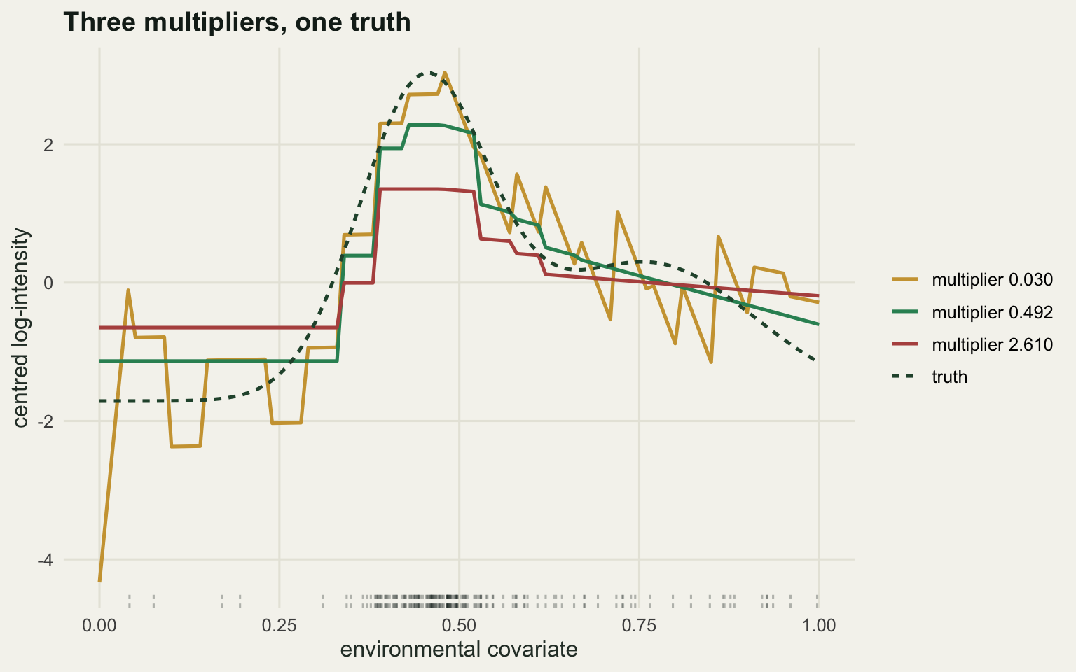
Sample size, and the rule the software encodes
The sqrt(m) in the penalty scale is a claim: that the right amount of shrinkage falls as the square root of the number of presence records, so that a fixed multiplier stays appropriate as the dataset grows. If that claim held exactly, the held-out-optimal multiplier would be flat in sample size. It is testable. I sweep the multiplier at five sample sizes with three replicate datasets each, average the held-out curves over replicates before taking the maximum, and interpolate the peak with a local parabola in log-multiplier.
spec_mid <- make_spec(c("linear", "quadratic", "hinge"), 10)
cat("mid basis features:", ncol(spec_mid$bg), "\n")
mid basis features: 44 size_grid <- c(25, 50, 100, 200, 400)
mult_grid <- 10^seq(-2.4, 0.8, length.out = 10)
nrep_size <- 3
cat("sample sizes:", paste(size_grid, collapse = " "), " replicates each:", nrep_size,
" multipliers:", length(mult_grid), "\n")sample sizes: 25 50 100 200 400 replicates each: 3 multipliers: 10 set.seed(4242)
size_tab <- NULL
size_curves <- matrix(0, length(size_grid), length(mult_grid))
for (si in seq_along(size_grid)) {
nrec <- size_grid[si]
acc <- matrix(0, nrep_size, length(mult_grid))
for (r in seq_len(nrep_size)) {
idx <- draw_records(nrec)
ff <- path_fit(spec_mid, idx, mult_grid, n_iter = 140)
acc[r, ] <- sapply(ff, function(z) mean(log_density(spec_mid, z$bhat)[eval_rec]))
}
avg <- colMeans(acc); size_curves[si, ] <- avg
kk <- which.max(avg); lgs <- log10(mult_grid)
if (kk > 1 && kk < length(mult_grid)) {
y1 <- avg[kk - 1]; y2 <- avg[kk]; y3 <- avg[kk + 1]
lbest <- lgs[kk] + 0.5 * (y1 - y3) / (y1 - 2 * y2 + y3) * (lgs[2] - lgs[1])
} else lbest <- lgs[kk]
within <- mult_grid[avg > max(avg) - 0.01]
size_tab <- rbind(size_tab, data.frame(records = nrec, best = 10^lbest, peak = max(avg),
flat_lo = min(within), flat_hi = max(within),
width = max(within) / min(within)))
}
print(format(round(size_tab, 3), nsmall = 3), row.names = FALSE) records best peak flat_lo flat_hi width
25.000 0.251 0.753 0.239 0.239 1.000
50.000 0.279 0.788 0.239 0.541 2.268
100.000 0.132 0.838 0.046 0.239 5.142
200.000 0.120 0.882 0.105 0.239 2.268
400.000 0.081 0.901 0.020 0.105 5.142slope_fit <- lm(log10(best) ~ log10(records), data = size_tab)
cat("slope of log10 best multiplier on log10 records:", round(coef(slope_fit)[2], 3), "\n")slope of log10 best multiplier on log10 records: -0.449 cat("implied penalty exponent (0.5 means the square-root rule):",
round(0.5 - coef(slope_fit)[2], 3), "\n")implied penalty exponent (0.5 means the square-root rule): 0.949 transfer <- approx(log10(mult_grid), size_curves[5, ], log10(size_tab$best[1]))$y
cat("held-out cost at 400 records of using the 25-record optimum:",
round(size_tab$peak[5] - transfer, 4), "\n")held-out cost at 400 records of using the 25-record optimum: 0.0153 The optimal multiplier is not flat. It falls from 0.251 at 25 records to 0.081 at 400, and the slope of its logarithm against the logarithm of sample size is -0.449. Since the encoded penalty already carries a factor of 1 / sqrt(m), that slope implies the total penalty should fall as m^-0.949, near one over the sample size rather than one over its square root. My measurement does not reproduce the rule the software encodes.
Before treating that as a finding to act on, look at the width column. On this run, at 25 records everything within 0.01 nats of the peak sits at a single grid value; at 400 records the same tolerance covers a factor of 5. The optimum flattens as data accumulate, which is exactly what should happen, and it means the disagreement is cheap: using the 25-record optimum on 400 records costs 0.0153 nats. The square-root rule is measurably wrong here and practically almost harmless, and those two statements are both worth having.
Feature classes at their own best multiplier
Comparing feature classes at a common multiplier is not a fair comparison, because the classes differ in dimension and therefore in how much shrinkage they need. So each class gets its own sweep and its own best multiplier, chosen on held-out data, and I record two things at that multiplier: the held-out likelihood, and the root mean squared distance between the fitted and the true response curve on the 101-point grid. A flat curve scores 1.424 on that second measure, so anything near that has recovered nothing.
class_specs <- list("linear" = make_spec("linear", 0),
                    "linear + quadratic" = make_spec(c("linear", "quadratic"), 0),
                    "hinge" = make_spec("hinge", 10),
                    "everything" = make_spec(c("linear", "quadratic", "product",
                                               "threshold", "hinge"), 10))
cat("features per class:",
    paste(names(class_specs), sapply(class_specs, function(z) ncol(z$bg)),
          collapse = "; "), "\n")
features per class: linear 2; linear + quadratic 4; hinge 40; everything 65 class_mults <- 10^seq(-2.4, 0.8, length.out = 8)
nrep_class <- 3
set.seed(808)
class_raw <- NULL
for (nrec in c(40, 400)) for (r in seq_len(nrep_class)) {
idx <- draw_records(nrec)
for (nm in names(class_specs)) {
sp <- class_specs[[nm]]
ff <- path_fit(sp, idx, class_mults, n_iter = 140)
hv <- sapply(ff, function(z) mean(log_density(sp, z$bhat)[eval_rec]))
kk <- which.max(hv)
class_raw <- rbind(class_raw,
data.frame(records = nrec, cls = nm, best = class_mults[kk], held_out = hv[kk],
shape = shape_err(resp_curve(sp, ff[[kk]]$bhat)),
nonzero = sum(ff[[kk]]$bhat != 0)))
}
}
class_tab <- aggregate(cbind(held_out, shape, nonzero, best) ~ cls + records,
class_raw, FUN = mean)
class_tab <- class_tab[order(class_tab$records, -class_tab$held_out), ]
print(format(class_tab, digits = 3), row.names = FALSE) cls records held_out shape nonzero best
hinge 40 0.80606 0.896 10.00 0.21006
everything 40 0.79063 0.641 14.67 0.26827
linear + quadratic 40 0.57753 1.123 3.67 0.03387
linear 40 0.00857 1.416 2.00 0.12196
hinge 400 0.90883 0.376 17.33 0.07332
everything 400 0.90223 0.384 34.00 0.07332
linear + quadratic 400 0.60486 1.428 4.00 0.04343
linear 400 0.01572 1.437 2.00 0.00398On this run, with 40 records, the hinge basis has the best held-out likelihood, 0.806, but the class that recovers the true shape best is everything, at 0.641 against the hinge basis’s 0.896. The two questions have different answers on the same fits: the model you would pick for prediction need not be the model you would quote a response curve from. At 400 records the two converge, 0.909 against 0.902 on held-out likelihood and 0.376 against 0.384 on shape.
I expected the restrictive class to win at the small sample size, in the usual way that bias beats variance when data are scarce. It did not, at either size. Linear and quadratic features together reach 0.578 at 40 records and 0.605 at 400, and that second number is close to the best they will ever do: it is a bias floor, not a sampling problem. The hinge basis at 40 records, 0.806, is already well above the quadratic ceiling at 400. A quadratic response curve is symmetric with one scale of curvature, and the true peak here is narrow with a shoulder, so no amount of data rescues it. The bias-beats-variance result requires the restrictive class to be nearly right, and that is an assumption about the species, not a general property of small samples. Linear features alone score 0.009 and 0.016, which is a uniform map with extra steps.
cls_long <- rbind(
  data.frame(cls = class_tab$cls, records = class_tab$records, val = class_tab$held_out,
             panel = "held-out log-likelihood (nats per record)"),
  data.frame(cls = class_tab$cls, records = class_tab$records, val = class_tab$shape,
             panel = "error in the recovered response shape"))
cls_ord <- c("linear", "linear + quadratic", "hinge", "everything")
panel_ord <- c("held-out log-likelihood (nats per record)",
               "error in the recovered response shape")
cls_long$cls <- factor(cls_long$cls, levels = cls_ord)
cls_long$panel <- factor(cls_long$panel, levels = panel_ord)
cls_long$per_n <- paste(cls_long$records, "records")
p_class <- ggplot(cls_long, aes(val, cls, fill = cls)) +
  geom_col(width = 0.65) +
  facet_grid(per_n ~ panel, scales = "free_x") +
  scale_fill_manual(values = c("linear" = te_pal$sage, "linear + quadratic" = te_pal$gold,
                               "hinge" = te_pal$green, "everything" = te_pal$forest)) +
  labs(x = NULL, y = NULL, title = "Each class at its own best multiplier") +
  theme_te() +
  theme(legend.position = "none", panel.spacing.x = unit(1.2, "lines"))
p_class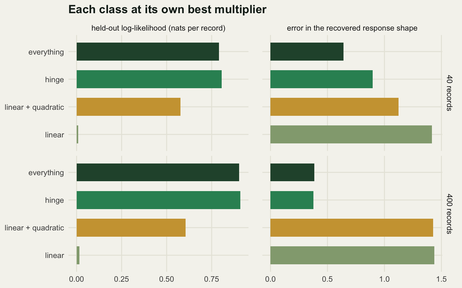
What the path cannot tell you
Everything above chose the multiplier on 4000 held-out records, which no one has. The realistic version is a split of the records you own, and if the number you tune on is also the number you report, the report is biased upwards. Here is the size of that bias: 30 replicate datasets of 120 records, split 80 for fitting and 40 for tuning, with the same fitted models scored again on the independent evaluation set.
spec_one <- make_spec(c("linear", "quadratic", "hinge"), 10, one_var = TRUE)
cat("single-covariate basis features:", ncol(spec_one$bg), "\n")
single-covariate basis features: 22 trap_mults <- 10^seq(-2, 0.8, length.out = 8)
nrep_trap <- 30
fixed_k <- 4
cat("replicates:", nrep_trap, " records each: 120 fitting: 80 tuning: 40\n")replicates: 30 records each: 120 fitting: 80 tuning: 40set.seed(31415)
shown <- numeric(nrep_trap); honest <- numeric(nrep_trap)
ctrl <- numeric(nrep_trap); picked <- numeric(nrep_trap)
for (r in seq_len(nrep_trap)) {
idx <- draw_records(120)
inner <- idx[1:80]; valid <- idx[81:120]
ff <- path_fit(spec_one, inner, trap_mults, n_iter = 120)
lds <- lapply(ff, function(z) log_density(spec_one, z$bhat))
vv <- sapply(lds, function(z) mean(z[valid]))
oo <- sapply(lds, function(z) mean(z[eval_rec]))
kk <- which.max(vv)
shown[r] <- vv[kk]; honest[r] <- oo[kk]; picked[r] <- trap_mults[kk]
ctrl[r] <- vv[fixed_k] - oo[fixed_k]
}
gap <- shown - honest
cat("mean tuning-split likelihood as reported:", round(mean(shown), 4), "\n")mean tuning-split likelihood as reported: 0.8981 cat("mean likelihood of the same fits on fresh records:", round(mean(honest), 4), "\n")mean likelihood of the same fits on fresh records: 0.8425 cat("raw optimism:", round(mean(gap), 4),
" standard error:", round(sd(gap) / sqrt(nrep_trap), 4), "\n")raw optimism: 0.0556 standard error: 0.0427 cat("same gap at a fixed multiplier:", round(mean(ctrl), 4),
" standard error:", round(sd(ctrl) / sqrt(nrep_trap), 4), "\n")same gap at a fixed multiplier: 0.009 standard error: 0.0407 cat("selection excess, paired:", round(mean(gap - ctrl), 4),
" standard error:", round(sd(gap - ctrl) / sqrt(nrep_trap), 4), "\n")selection excess, paired: 0.0466 standard error: 0.009 cat("spread of one tuning estimate across replicates (sd):", round(sd(shown), 3), "\n")spread of one tuning estimate across replicates (sd): 0.238 cat("multipliers chosen, 10th to 90th percentile:",
paste(round(quantile(picked, c(0.1, 0.9)), 3), collapse = " to "),
" distinct values:", length(unique(picked)), "\n")multipliers chosen, 10th to 90th percentile: 0.01 to 0.398 distinct values: 6 The tuned score people would report averages 0.8981; the same models on fresh records average 0.8425. The raw difference is 0.0556 with a standard error of 0.0427, which on its own does not separate the cost of choosing from the noise in the two scores. Subtracting the same difference measured at a fixed multiplier removes the shared noise of the small tuning split and isolates the part caused by choosing: 0.0466 nats with a standard error of 0.009. That is the selection bias, and it is real.
It is also smaller than the other problem in the same table. One tuning estimate varies with a standard deviation of 0.238 across replicates, five times the selection bias, and the chosen multiplier ranges from 0.01 to 0.398 between the tenth and ninetieth percentiles, taking 6 distinct values out of 8 offered. A 40-record tuning split does not locate the optimum; treat what it returns as a rough setting rather than an estimate. Report the tuned score on a nested split, as in Data leakage in model validation, but do not expect the tuned multiplier itself to be reproducible.
Two more limits, and the first is a property of the penalty rather than of this simulation. Adjacent hinge features are near copies of each other, and L1 keeps one of a correlated group and drops the rest, with the choice depending on the sample.
pair <- c(8, 9)
cat("knots of the pair:", round(spec_mid$knots[pair - 4], 3), "\n")
knots of the pair: 0.364 0.455 cat("correlation between the two adjacent hinge features:",
round(cor(spec_mid$bg[, pair[1]], spec_mid$bg[, pair[2]]), 3), "\n")correlation between the two adjacent hinge features: 0.99 fwd <- 5:14
set.seed(606)
sel <- matrix(FALSE, 25, length(fwd))
for (r in 1:25) {
idx <- draw_records(40)
ft <- fit_maxent(spec_mid, colMeans(spec_mid$bg[idx, ]),
0.16 * spec_mid$pen / sqrt(40), n_iter = 160)
sel[r, ] <- ft$bhat[fwd] != 0
}
print(rbind(knot = round(spec_mid$knots, 2), kept = colSums(sel))) [,1] [,2] [,3] [,4] [,5] [,6] [,7] [,8] [,9] [,10]
knot 0.09 0.18 0.27 0.36 0.45 0.55 0.64 0.73 0.82 0.91
kept 0.00 0.00 0.00 0.00 25.00 0.00 9.00 8.00 9.00 10.00cat("distinct selected sets among 25 fits:", nrow(unique(sel)), "\n")distinct selected sets among 25 fits: 11 Two adjacent forward hinges correlate at 0.99. Across 25 datasets of 40 records the hinge at knot 0.45, the one sitting on the true peak, is kept every time, so the penalty is not indiscriminate. The four hinges in the upper tail are another matter: each is kept in 8 to 10 of the 25 fits, and the 25 fits produce 11 distinct selected sets. A feature missing from your MaxEnt output is not evidence that the covariate does not matter there. It may only mean that a near copy of it got in first.
The second limit is larger and no part of the path can see it. Regularisation controls flexibility, not correctness. Every number in this tutorial was computed by comparing a model to records drawn from the same process that generated the training records, so the held-out likelihood measures agreement with the record-generating process, not with the species. If the records are concentrated along roads and rivers, the held-out records are too, the path will find its interior optimum exactly as it did here, and the result will be a well-tuned smooth map of survey effort. A heavily penalised model fitted to biased records is a smooth statement about where people looked. Nothing in the multiplier, and no amount of held-out data drawn the same way, can tell you which of the two you have.
Where to go next
The next tutorial in this cluster takes on the problem this one cannot: Sampling bias in presence-only models, where the records are drawn with an effort surface layered on top of the intensity, and the fix has to come from the background sample or from an explicit effort term rather than from the penalty. After that, Checking a presence-only model covers what to check on a fitted model before you believe its map.
References
Phillips SJ, Dudik M 2008 Ecography 31(2):161-175 (10.1111/j.0906-7590.2008.5203.x)
Merow C, Smith MJ, Silander JA 2013 Ecography 36(10):1058-1069 (10.1111/j.1600-0587.2013.07872.x)
Muscarella R, Galante PJ, Soley-Guardia M, Boria RA, Kass JM, Uriarte M, Anderson RP 2014 Methods in Ecology and Evolution 5(11):1198-1205 (10.1111/2041-210X.12261)
Radosavljevic A, Anderson RP 2014 Journal of Biogeography 41(4):629-643 (10.1111/jbi.12227)
Renner IW, Warton DI 2013 Biometrics 69(1):274-281 (10.1111/j.1541-0420.2012.01824.x)
Tibshirani R 1996 Journal of the Royal Statistical Society Series B 58(1):267-288 (10.1111/j.2517-6161.1996.tb02080.x)