library(ggplot2)
library(patchwork)

te_paper  <- "#f5f4ee"
te_ink    <- "#16241d"
te_body   <- "#2c3a31"
te_forest <- "#275139"
te_rust   <- "#b5534e"
te_gold   <- "#c9b458"
te_line   <- "#dad9ca"

theme_datasheet <- function() {
  theme_minimal(base_size = 12) +
    theme(plot.background  = element_rect(fill = te_paper, colour = NA),
          panel.background = element_rect(fill = te_paper, colour = NA),
          panel.grid.major = element_line(colour = te_line, linewidth = 0.3),
          panel.grid.minor = element_blank(),
          text             = element_text(colour = te_body),
          plot.title       = element_text(colour = te_ink, face = "bold"),
          plot.subtitle    = element_text(colour = te_body),
          axis.text        = element_text(colour = te_body),
          strip.text       = element_text(colour = te_ink))
}The mid-domain effect as a null for richness
R
macroecology
null models
species richness
simulation
ecology tutorial
A range-shuffling mid-domain null fits a central environmental hump with r-squared near 0.9. An envelope and a species midpoint test in R tell geometry apart.
An elevational survey of moths on a mountain in the Carpathians is summarised the way most such surveys are: the slope is cut into bands of equal height, every species is given a range from its lowest to its highest record, and richness is counted per band. The count peaks halfway up. The discussion section offers a temperature and moisture optimum at mid elevation, and a reviewer replies with one sentence: have you ruled out the mid-domain effect?
The reviewer’s point goes back to Colwell and Hurtt (1994), who placed ranges at random between two hard boundaries, with no environment in the model at all, and still got richness peaking in the middle, because a range of any size placed inside a bounded domain overlaps the centre more often than the edges. Colwell and Lees (2000) named it the mid-domain effect and reviewed the models built on it. The version most often run keeps every observed range extent, moves each range to a random position where it still fits inside the domain, recounts richness and repeats. Zapata, Gaston and Chown (2003) called the assumptions of these models unrealistic or internally inconsistent and listed problems with how they are tested, among them collapsing two dimensions to one, interpolated ranges, and deviation measures that are insensitive and prone to Type I error when the data are spatially autocorrelated. Connolly (2005) built process-based models of range placement and argued that the randomisation probably overstates how much of a real pattern geometry explains. None of the results below is new. The post runs that null on simulated domains whose truth is known and asks which summary of it can tell geometry from an environmental hump, which is the question the reviewer’s sentence leaves open.
The usual way to answer is to correlate observed band richness with the mean of the null and quote the r-squared. The sections below lead instead with two summaries that do discriminate, the share of bands that fall inside the null’s 95 per cent envelope and a test on species midpoints, and then show why the r-squared on its own reads as support for geometry in worlds that have none.
Three posts on this site run nulls that sit close to this one. In Checking a macroecological pattern the null for the abundance-occupancy slope keeps each species’ record total and scatters the records over grid cells; there is no range and no domain edge in it. Elements of metacommunity structure: a stress test builds a null that keeps range lengths and contiguity and places ranges at random along an ordination axis, which is the same shuffle, but it is used to judge whether range boundaries clump, not what richness the placement implies. Range size distributions asks what the shape of the range size distribution is evidence for and never asks where on the map the ranges sit. Here the range sizes are taken as given and only their positions are in question.
A domain with two hard edges
The domain is the unit interval with hard edges at 0 and 1, cut into 40 bands of equal width. A regional pool of 250 species is simulated in every world. A species has a true range extent drawn from a Beta distribution, either Beta(1, 3), mostly narrow ranges with a mean of a quarter of the domain, or Beta(2, 2), wider ranges with a mean of half. It is present in a band when its range covers the band’s midpoint.
Where a range sits depends on the truth of the world. Under geometry only, the midpoint is uniform over the positions where the whole range fits, which is exactly what the null assumes. Under a monotone gradient the midpoints are Beta(1, 3), piled towards the lower edge. Under a central optimum the midpoints are normal around the centre with standard deviation 0.15, a species’ environmental optimum in the middle of the domain and nothing geometric about it. In the two environmental worlds a range that runs past an edge is cut off there, so the observed extent is shorter than the true one; that clipped extent is what a survey would record and what the null is given. A fourth world mixes geometry and the central optimum species by species. All of these constants, the 300 worlds per cell and the 199 null placements per world were fixed before the first run.
Each world is scored four ways. The r-squared is the squared correlation between observed band richness and the mean of the 199 null placements. The envelope share is the share of the 40 bands whose observed richness lies between the 5th and 195th of the 199 sorted null values, a pointwise 95 per cent envelope. The species test uses the fact that under the null each midpoint is uniform on its own feasible interval, so its position within that interval, (midpoint minus half the extent) divided by (one minus the extent), is uniform on 0 to 1 whatever the extent. A one-sample Kolmogorov-Smirnov test of those positions against the uniform is a test of the null that uses species, not bands. A range clipped at an edge has a position of exactly 0 or 1, and ks.test() warns about ties; the null itself puts no mass there, so the ties are part of the evidence rather than a violation, and the code moves them by less than a billionth, which changes the statistic by less than that and silences the warning. The last score is a band-level correlation with a covariate, taken up further down.
The engine counts band richness with a difference array instead of a species by band comparison, so one call handles all 199 null placements of a world at once. The envelope sorts band by band in a single sort() by adding a large offset per band.
n_sp     <- 250     # species in the regional pool
n_band   <- 40      # bands along the domain
n_null   <- 199     # null placements per world
n_world  <- 300     # simulated worlds per cell
alpha    <- 0.05
opt_sd   <- 0.15    # spread of midpoints around a central optimum
ext_sets <- list("Beta(1, 3)" = c(1, 3), "Beta(2, 2)" = c(2, 2))
band_mid <- (seq_len(n_band) - 0.5) / n_band

# richness per band for many sets of ranges at once (species in rows, sets in columns)
band_rich <- function(lo, hi) {
  n_set <- ncol(lo)
  first <- pmax(ceiling(lo * n_band + 0.5), 1)
  last  <- pmin(floor(hi * n_band + 0.5), n_band)
  ok    <- first <= last
  off   <- (col(lo) - 1) * (n_band + 1)
  step  <- tabulate((off + first)[ok], n_set * (n_band + 1)) -
    tabulate((off + last + 1)[ok], n_set * (n_band + 1))
  apply(matrix(step, n_band + 1), 2, cumsum)[seq_len(n_band), , drop = FALSE]
}

# Colwell-Lees null: keep each extent, draw its midpoint uniformly where it fits
null_envelope <- function(lo, hi) {
  ext   <- hi - lo
  mid0  <- ext / 2 + matrix(runif(n_sp * n_null), n_sp) * (1 - ext)
  nullr <- band_rich(mid0 - ext / 2, mid0 + ext / 2)
  offb  <- rep((seq_len(n_band) - 1) * 1000, n_null)
  srt   <- matrix(sort(nullr + offb) - sort(offb), ncol = n_band)
  list(lo = srt[5, ], hi = srt[195, ], mean = rowMeans(nullr), nullr = nullr)
}

# species-level test: where each midpoint sits inside its own feasible interval
pit_test <- function(lo, hi, keep = TRUE) {
  ext  <- hi - lo
  use  <- ext < 1 - 1e-9 & keep
  pit  <- ((lo + hi) / 2 - ext / 2)[use] / (1 - ext[use])
  n_u  <- length(pit)
  pit  <- pmin(pmax(pit, runif(n_u, 0, 1e-9)), 1 - runif(n_u, 0, 1e-9))
  ks.test(pit, "punif", exact = FALSE)$p.value
}

central_mid <- function(n) pmin(pmax(rnorm(n, 0.5, opt_sd), 0), 1)

one_world <- function(truth, shape, w_mde = 1, extras = TRUE) {
  ext_true <- rbeta(n_sp, shape[1], shape[2])
  feasible <- runif(n_sp, ext_true / 2, 1 - ext_true / 2)
  mid <- switch(truth,
                mde     = feasible,
                mono    = rbeta(n_sp, 1, 3),
                central = central_mid(n_sp),
                mix     = ifelse(runif(n_sp) < w_mde, feasible, central_mid(n_sp)))
  lo  <- pmax(mid - ext_true / 2, 0)
  hi  <- pmin(mid + ext_true / 2, 1)
  obs <- band_rich(cbind(lo), cbind(hi))[, 1]
  env <- null_envelope(lo, hi)
  r2_o <- cor(obs, env$mean)^2
  in_o <- mean(obs >= env$lo & obs <= env$hi)
  # the same two scores for every null placement, against the same mean and envelope
  r2_n <- cor(env$nullr, env$mean)[, 1]^2
  in_n <- colMeans(env$nullr >= env$lo & env$nullr <= env$hi)
  core <- c(r2       = r2_o,
            inside   = in_o,
            rej      = pit_test(lo, hi) < alpha,
            rej_env  = (1 + sum(in_n <= in_o)) / (n_null + 1) < alpha,
            rej_r2   = (1 + sum(r2_n <= r2_o)) / (n_null + 1) < alpha)
  if (!extras) return(core)
  env_true <- null_envelope(0.5 - ext_true / 2, 0.5 + ext_true / 2)
  clip  <- lo <= 0 | hi >= 1
  covar <- sin(2 * pi * (runif(1, 0.5, 1.5) * band_mid + runif(1)))
  c(core,
    inside_true = mean(obs >= env_true$lo & obs <= env_true$hi),
    below       = mean(obs < env$lo),
    below_true  = mean(obs < env_true$lo),
    above       = mean(obs > env$hi),
    above_true  = mean(obs > env_true$hi),
    tot_null    = sum(env$mean) / sum(obs),
    tot_true    = sum(env_true$mean) / sum(obs),
    rej_unclip  = pit_test(lo, hi, !clip) < alpha,
    clip        = mean(clip),
    cor_smooth  = cor.test(obs, covar)$p.value < alpha,
    cor_resid   = cor.test(obs - env$mean, covar)$p.value < alpha,
    cor_white   = cor.test(obs, rnorm(n_band))$p.value < alpha)
}
The expected hump has a closed form
Before any biology is added the null has an expected shape that needs no simulation. Take a range of extent r and a point x in the lower half of the domain. The range midpoint is uniform over an interval of length 1 - r, and the range covers x when the midpoint lies within r/2 of it and inside the feasible interval. The length of that overlap is r when r is at most x, x when r lies between x and 1 - x, and 1 - r beyond that, so it is min(r, x, 1 - x, 1 - r) in all cases and the chance of cover is that length divided by 1 - r. Integrating over the extent distribution gives the expected share of species in a band.
Two extent distributions give familiar curves. With uniform extents the integral is -x log x - (1 - x) log(1 - x), the entropy function, with a peak of log 2 in the middle. With Beta(1, 2) extents, which is what two range endpoints dropped independently at random produce, it is the parabola 2x(1 - x) with a peak of one half. The code checks both against numerical integration and all four curves against 20000 simulated species.
occ_exact <- function(x, a, b) {
  integrate(function(r) dbeta(r, a, b) * pmin(r, x, 1 - x, 1 - r) / (1 - r),
            0, 1, rel.tol = 1e-8)$value
}
calib_sets <- list("Beta(1, 1)" = c(1, 1), "Beta(1, 2)" = c(1, 2),
                   "Beta(1, 3)" = c(1, 3), "Beta(2, 2)" = c(2, 2))
n_calib <- 20000
set.seed(7301)
calib <- do.call(rbind, lapply(names(calib_sets), function(nm) {
  ab  <- calib_sets[[nm]]
  ext <- rbeta(n_calib, ab[1], ab[2])
  mid <- runif(n_calib, ext / 2, 1 - ext / 2)
  data.frame(extents = nm, x = band_mid,
             exact = vapply(band_mid, occ_exact, 0, a = ab[1], b = ab[2]),
             sim = band_rich(cbind(mid - ext / 2), cbind(mid + ext / 2))[, 1] / n_calib)
}))
entropy <- function(x) -x * log(x) - (1 - x) * log(1 - x)
cpick <- function(nm, band) calib$exact[calib$extents == nm][band]
gap_entropy  <- max(abs(calib$exact[calib$extents == "Beta(1, 1)"] - entropy(band_mid)))
gap_parabola <- max(abs(calib$exact[calib$extents == "Beta(1, 2)"] - 2 * band_mid * (1 - band_mid)))
gap_sim  <- max(abs(calib$sim - calib$exact))
se_worst <- sqrt(0.25 / n_calib)
ratio_dev <- max(abs(calib$exact[calib$extents == "Beta(2, 2)"] /
                     calib$exact[calib$extents == "Beta(1, 3)"] - 2))
The numerical integral for uniform extents differs from the entropy curve by at most 1.90e-11 over the 40 band midpoints, and the Beta(1, 2) integral differs from the parabola by at most 2.11e-11. At the centre band the expected share is 0.693 for uniform extents, 0.500 for Beta(1, 2), 0.375 for Beta(1, 3) and 0.750 for Beta(2, 2); in the edge band it is 0.067, 0.025, 0.019 and 0.037. The simulated shares differ from the integral by at most 0.0076 in any of the 160 band and distribution pairs, where one binomial standard error is at most 0.0035. The null hump is set by the extent distribution alone, and no parameter of the placement enters. Wider ranges raise it without always changing its shape: the Beta(2, 2) curve is twice the Beta(1, 3) curve in every band (the ratio differs from 2 by at most 6.48e-10), because the overlap length min(r, x, 1 - x, 1 - r) is unchanged when r is replaced by 1 - r, and under that swap the Beta(2, 2) integrand becomes exactly twice the Beta(1, 3) one. The two extent sets used below therefore give expected null curves of the same shape.
ggplot(calib, aes(x, exact, colour = extents)) +
  geom_line(aes(linetype = extents), linewidth = 0.9) +
  geom_point(aes(y = sim), size = 1.4, alpha = 0.8) +
  scale_linetype_manual(values = c("Beta(1, 1)" = "22", "Beta(1, 2)" = "solid",
                                   "Beta(1, 3)" = "solid", "Beta(2, 2)" = "solid"),
                        name = "range extents") +
  scale_colour_manual(values = c("Beta(1, 1)" = te_ink, "Beta(1, 2)" = te_gold,
                                 "Beta(1, 3)" = te_rust, "Beta(2, 2)" = te_forest),
                      name = "range extents") +
  labs(x = "position in the domain", y = "share of species covering the band",
       title = "The mid-domain hump before any biology",
       subtitle = "lines: exact integral; points: 20000 simulated species") +
  theme_datasheet() +
  theme(legend.position = "bottom")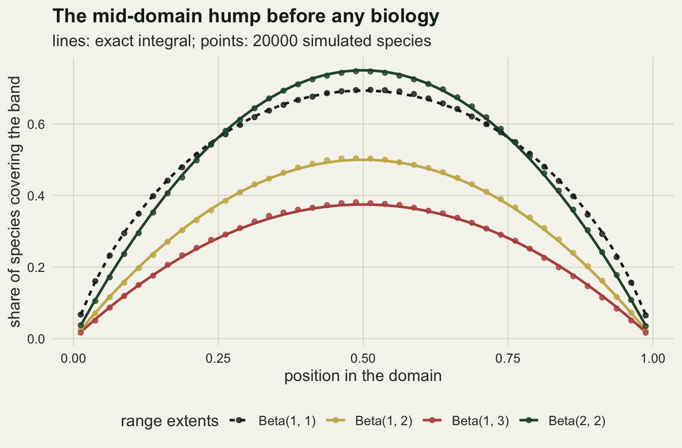
Four worlds and one null
One world of each pure truth, all with Beta(1, 3) extents, shows what the null does with each.
set.seed(4417)
truth_lab <- c(mde = "geometry only", mono = "monotone gradient", central = "central optimum")
ex <- do.call(rbind, lapply(names(truth_lab), function(tr) {
  ext_true <- rbeta(n_sp, 1, 3)
  mid <- switch(tr, mde = runif(n_sp, ext_true / 2, 1 - ext_true / 2),
                mono = rbeta(n_sp, 1, 3), central = central_mid(n_sp))
  lo  <- pmax(mid - ext_true / 2, 0)
  hi  <- pmin(mid + ext_true / 2, 1)
  obs <- band_rich(cbind(lo), cbind(hi))[, 1]
  env <- null_envelope(lo, hi)
  data.frame(truth = tr, x = band_mid, obs = obs, lo = env$lo, hi = env$hi, nm = env$mean,
             r2 = cor(obs, env$mean)^2, inside = mean(obs >= env$lo & obs <= env$hi),
             p_sp = pit_test(lo, hi))
}))
ex_stat <- unique(ex[, c("truth", "r2", "inside", "p_sp")])
epick <- function(tr, col) ex_stat[ex_stat$truth == tr, col]
Under geometry only the r-squared is 0.968, 40 of the 40 bands lie inside the envelope and the species test gives p = 0.666. Under the central optimum the r-squared is still 0.860, but only 17 bands lie inside, and the species test gives p = 7.39e-06. The monotone gradient is not a hump and fails every score: r-squared 0.0006, 4 bands inside, p < 1.00e-15. In the central panel the observed hump is narrower and taller than the null’s: too many species in the middle bands and too few on the shoulders, which an uncalibrated correlation does not register and an envelope shows band by band.
ex$panel <- factor(sprintf("%s\nr2 %.2f, %d of %d bands inside", truth_lab[ex$truth],
                           ex$r2, round(ex$inside * n_band), n_band),
                   levels = unique(sprintf("%s\nr2 %.2f, %d of %d bands inside",
                                           truth_lab[ex$truth], ex$r2,
                                           round(ex$inside * n_band), n_band)))
ex$out <- ex$obs < ex$lo | ex$obs > ex$hi
ggplot(ex, aes(x)) +
  geom_ribbon(aes(ymin = lo, ymax = hi), fill = te_line) +
  geom_line(aes(y = nm), colour = te_forest, linewidth = 0.8) +
  geom_point(aes(y = obs, colour = out), size = 1.6) +
  scale_colour_manual(values = c("FALSE" = te_ink, "TRUE" = te_rust),
                      labels = c("inside the envelope", "outside"), name = NULL) +
  facet_wrap(~panel) +
  scale_x_continuous(breaks = c(0, 0.5, 1)) +
  labs(x = "position in the domain", y = "species per band",
       title = "Same null, three truths",
       subtitle = "250 species, Beta(1, 3) extents; grey: 95 per cent envelope of 199 null placements") +
  theme_datasheet() +
  theme(legend.position = "bottom", panel.spacing = unit(1.4, "lines"))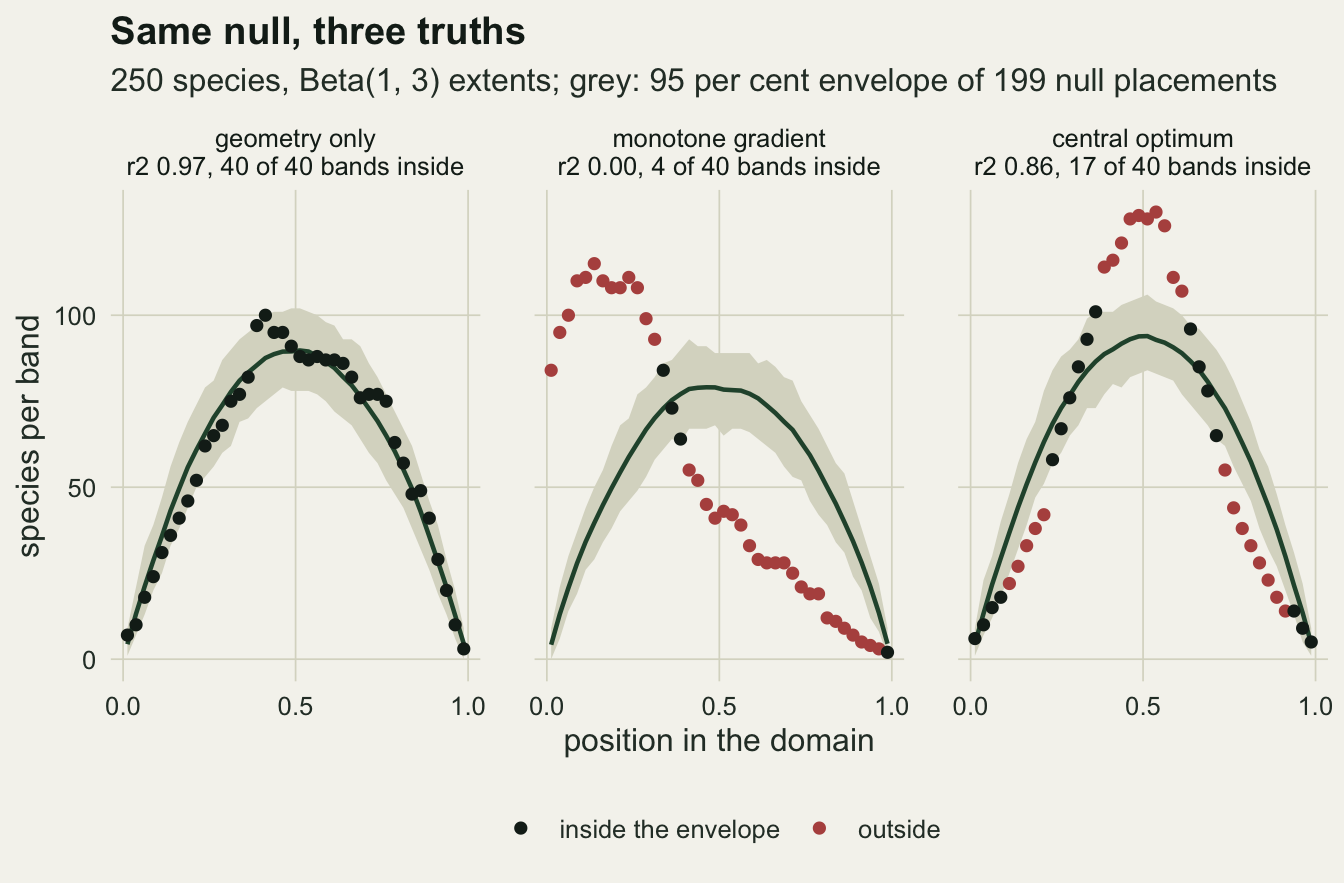
One world is an anecdote. The rest of the post runs 300 worlds for each of the three pure truths and both extent distributions.
set.seed(2003)
cells <- expand.grid(truth = c("mde", "mono", "central"), extents = names(ext_sets),
                     stringsAsFactors = FALSE)
sim_raw <- do.call(rbind, lapply(seq_len(nrow(cells)), function(i) {
  runs <- t(replicate(n_world, one_world(cells$truth[i], ext_sets[[cells$extents[i]]])))
  data.frame(truth = cells$truth[i], extents = cells$extents[i], runs)
}))
spick <- function(tr, ex_nm, col, f = mean) f(sim_raw[sim_raw$truth == tr & sim_raw$extents == ex_nm, col])
mc_se <- function(p) sqrt(p * (1 - p) / n_world)
shift <- function(tr, ex_nm) spick(tr, ex_nm, "inside") - spick(tr, ex_nm, "inside_true")
shift_se <- function(tr, ex_nm) {
  k <- sim_raw$truth == tr & sim_raw$extents == ex_nm
  sd(sim_raw$inside[k] - sim_raw$inside_true[k]) / sqrt(n_world)
}
The envelope and the species test
Under geometry only, the null holds as it should. The species test rejects in 0.040 of worlds with Beta(1, 3) extents and 0.027 with Beta(2, 2), against a nominal 0.05 and a Monte Carlo standard error of 0.013. The mean envelope share is 0.962 and 0.964, near the 0.95 a pointwise envelope promises.
Under the central optimum, the species test rejects in 1.000 of worlds with narrow ranges and 0.917 with wide ones, and under the monotone gradient in 1.000 and 1.000. Clipped ranges are not what drives it. The share of species clipped at an edge in central optimum worlds is 0.044 and 0.183, and rerunning the test on the unclipped species only gives rejection rates of 1.000 and 0.983: the midpoints are too central, and the test sees that without the edge ties.
The envelope share falls to a mean of 0.334 and 0.561 under the central optimum. A share is not a test until it has a reference distribution, and the null placements that built the envelope supply one. Each of the 199 placements has its own share of bands inside the same envelope, and the rank of the observed share among them gives a Monte Carlo p-value: one plus the number of placements with a share at or below the observed one, divided by 200. Under geometry only this rank test rejects in 0.047 of worlds with Beta(1, 3) extents and 0.040 with Beta(2, 2); under the central optimum it rejects in 1.000 and 0.990. A rule such as “most bands inside the envelope, so the null fits” is not that test: the central optimum worlds with wide ranges kept 0.561 of their bands inside on average.
What the r-squared does and does not say
The r-squared of observed richness against the null mean has a median of 0.873 in central optimum worlds with Beta(1, 3) extents and 0.955 with Beta(2, 2), and the share of those worlds above 0.5 is 1.000 and 1.000. Reported without a reference, a value near 0.9 reads as geometry explaining nearly all of the pattern, in worlds where geometry explains none of it. Any central hump correlates with any other central hump.
The medians under geometry only are higher, 0.970 and 0.993, and the r-squared can go through the same rank test as the envelope share: each null placement has its own r-squared against the null mean, and the observed value is ranked among those 199. That test rejects in 0.043 and 0.037 of geometry-only worlds and in 0.990 and 0.973 of central optimum worlds. In the pure worlds, then, the fault is not the r-squared as a statistic but reading it on an absolute scale. A high r-squared is what the null predicts; the question is whether it is as high as the null predicts, and that needs the same simulation the envelope uses. The mixed worlds below show where even the r-squared rank test falls behind.
The monotone gradient is the easy case for every score: median r-squared 0.0021 and 0.0205, mean envelope share 0.109 and 0.079.
sim_raw$truth_lab <- factor(truth_lab[sim_raw$truth], levels = truth_lab)
p_r2 <- ggplot(sim_raw, aes(r2, truth_lab)) +
  geom_boxplot(fill = te_line, colour = te_body, outlier.size = 0.6, width = 0.6) +
  facet_wrap(~extents, ncol = 1) +
  scale_x_continuous(breaks = c(0, 0.5, 1)) +
  labs(x = "r-squared against null mean", y = NULL, title = "Fit to the null") +
  theme_datasheet()
p_in <- ggplot(sim_raw, aes(inside, truth_lab)) +
  geom_boxplot(fill = te_line, colour = te_body, outlier.size = 0.6, width = 0.6) +
  facet_wrap(~extents, ncol = 1) +
  scale_x_continuous(breaks = c(0, 0.5, 1)) +
  labs(x = "share of bands inside", y = NULL, title = "Envelope") +
  theme_datasheet() +
  theme(axis.text.y = element_blank())
p_r2 + p_in + plot_annotation(theme = theme_datasheet())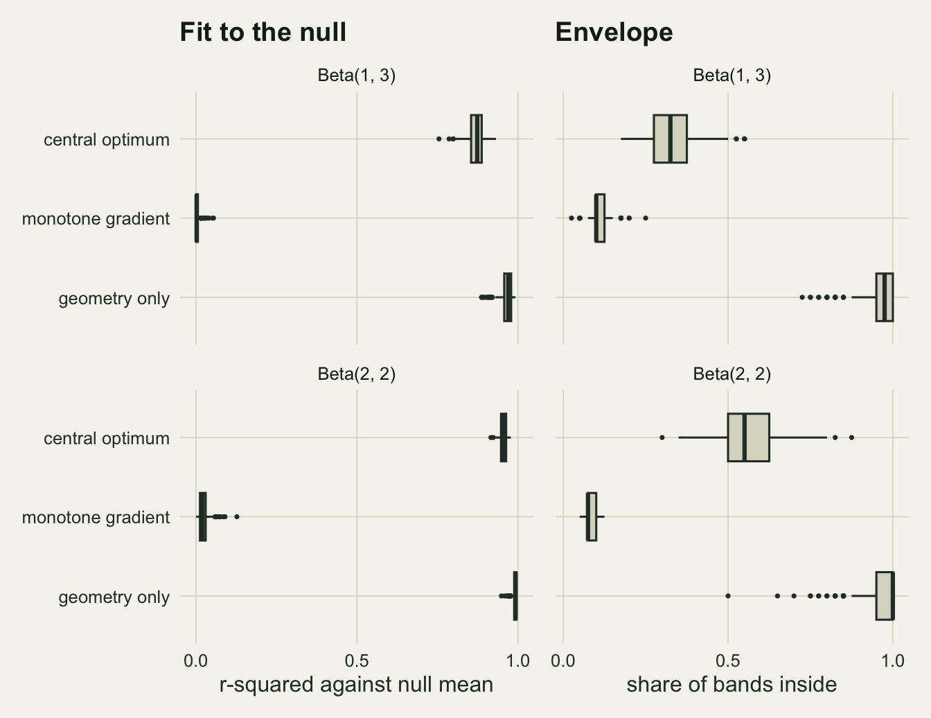
Worlds with both
Real assemblages are unlikely to be all geometry or all environment. In the mixed worlds each species is placed by the geometric null with probability w and around the central optimum otherwise, with Beta(1, 3) extents. The two band scores use the rank tests against their own 199 null placements, as above, and the species test needs no reference beyond the uniform. The endpoints w = 0 and w = 1 reuse the pure worlds.
set.seed(2005)
w_grid <- c(0.25, 0.5, 0.75, 0.9)
mix_raw <- do.call(rbind, lapply(w_grid, function(w) {
  runs <- t(replicate(n_world, one_world("mix", ext_sets[["Beta(1, 3)"]], w, extras = FALSE)))
  data.frame(w_mde = w, runs)
}))
ends <- rbind(data.frame(w_mde = 0, sim_raw[sim_raw$truth == "central" & sim_raw$extents == "Beta(1, 3)", colnames(mix_raw)[-1]]),
              data.frame(w_mde = 1, sim_raw[sim_raw$truth == "mde" & sim_raw$extents == "Beta(1, 3)", colnames(mix_raw)[-1]]))
mix_all <- rbind(mix_raw, ends)
mix_s <- data.frame(w_mde = sort(unique(mix_all$w_mde)))
mix_s$rej    <- tapply(mix_all$rej, mix_all$w_mde, mean)
mix_s$env    <- tapply(mix_all$rej_env, mix_all$w_mde, mean)
mix_s$r2cut  <- tapply(mix_all$rej_r2, mix_all$w_mde, mean)
# paired difference between the envelope rank test and the species test
mix_d <- function(w) {
  d <- mix_all$rej_env[mix_all$w_mde == w] - mix_all$rej[mix_all$w_mde == w]
  c(diff = mean(d), se = sd(d) / sqrt(length(d)))
}
mix_s$r2med  <- tapply(mix_all$r2, mix_all$w_mde, median)
mpick <- function(w, col) mix_s[mix_s$w_mde == w, col]
mix_long <- rbind(data.frame(w_mde = mix_s$w_mde, rate = mix_s$rej, rule = "species midpoint test"),
data.frame(w_mde = mix_s$w_mde, rate = mix_s$env, rule = "envelope share, rank test"),
data.frame(w_mde = mix_s$w_mde, rate = mix_s$r2cut, rule = "r-squared, rank test"))
mix_long$se <- sqrt(mix_long$rate * (1 - mix_long$rate) / n_world)
ggplot(mix_long, aes(w_mde, rate, colour = rule)) +
geom_hline(yintercept = alpha, linetype = "dashed", colour = te_body) +
geom_line(linewidth = 0.9) +
geom_errorbar(aes(ymin = rate - 2 * se, ymax = rate + 2 * se), width = 0.02) +
geom_point(size = 2) +
scale_colour_manual(values = c("species midpoint test" = te_forest,
"envelope share, rank test" = te_gold,
"r-squared, rank test" = te_rust), name = NULL) +
labs(x = "share of species placed by geometry alone", y = "rejection rate of the null",
title = "How much environment the tests can see",
subtitle = "Beta(1, 3) extents, 300 worlds per point, bars two Monte Carlo standard errors") +
theme_datasheet() +
theme(legend.position = "bottom")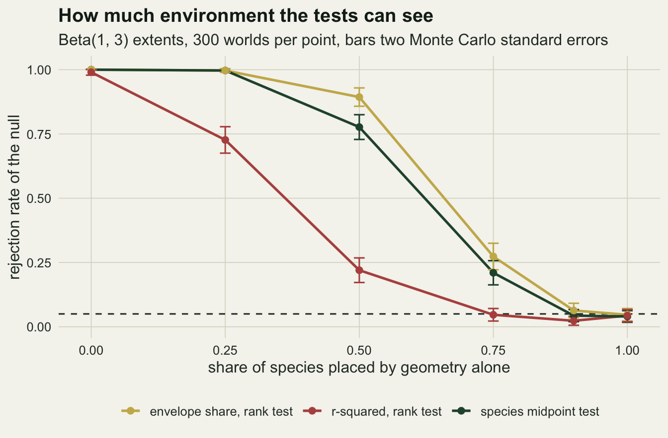
With half the species placed by geometry, the species test rejects in 0.777 of worlds, the envelope rank test in 0.893 and the r-squared rank test in 0.220. At three quarters geometry the rates are 0.210, 0.273 and 0.047, and at 0.9 they are 0.043, 0.063 and 0.023, with a Monte Carlo standard error of about 0.025 near a rate of one quarter. The r-squared loses the environmental species first. Its median climbs from 0.873 with no geometric species to 0.937 at one half, and reaches 0.961 with a quarter of the species placed by the environment, where the r-squared rank test rejects in 0.047 of worlds against 0.043 in worlds with no environmental species, a gap smaller than one Monte Carlo standard error. The envelope rank test rejects more often than the species test at one half and at three quarters, by 0.117 (paired standard error 0.025) and 0.063 (0.027), and it uses nothing the species test does not have: the observed ranges and their null placements. Neither sees a small environmental share: at w = 0.9 both are within two standard errors of the 0.05 they would give with none.
This is the reply to anyone who wants the mixture weight itself. The sweep gives power at known weights, not an estimate of w for a given assemblage. Estimating it needs a model of where the non-geometric species sit, and the central normal here is one invented shape; with the wrong shape the fitted weight would absorb the error. That is the route Connolly (2005) takes with process-based models, and it is a modelling question the randomisation cannot settle.
Bands are not replicates
Once the null has been run, the next step in many papers is to correlate band richness, or richness minus the null expectation, with an environmental variable measured per band and to quote the p-value with 38 degrees of freedom. Zapata and colleagues (2003) warned that such tests are prone to Type I error in spatially autocorrelated data; the simulation puts a size on it. Neighbouring bands share most of their species, so richness is a smooth curve along the domain, and a smooth curve correlates with any other smooth curve more often than an independent sample of 40 would.
Each geometry-only world above also drew a covariate that has nothing to do with richness: a sine wave with a random phase and between half a cycle and one and a half cycles across the domain, the kind of shape a temperature or rainfall profile has. Richness did not depend on it in any world. cor.test() of richness against it was significant at 0.05 in 0.723 of worlds with Beta(1, 3) extents and 0.767 with Beta(2, 2). Subtracting the null mean first, the residual approach, still gave 0.563 and 0.557, because the residual curve is as smooth as the richness curve. Against a covariate of independent normal values per band the rates were 0.033 and 0.057. The inflation needs both series to be smooth, and real environmental profiles along a gradient are. The 40 bands are not 40 replicates, and removing the geometric expectation does not make them so.
Observed extents in the null
The randomisation takes range sizes as observed, although the observed sizes were produced by the same domain and the same environment the test is meant to judge, which critics of mid-domain models have treated as circular. In the simulation the true extents are known, so the environmental worlds were also scored against an envelope built from the true, unclipped extents. Under geometry only the two envelopes are the same, because nothing is clipped.
The comparison is the share of bands inside the observed-extent envelope minus the share inside the true-extent one, paired world by world. With the central optimum and Beta(1, 3) extents, 0.044 of species are clipped and the shares are 0.334 and 0.320 (a shift of 0.013, standard error 0.002); with Beta(2, 2) extents, 0.183 clipped, they are 0.561 and 0.457 (shift 0.105, standard error 0.004). Under the monotone gradient more species are clipped, 0.310 and 0.574, yet the shifts are 0.013 (shares 0.109 and 0.096, standard error 0.002) and 0.009 (shares 0.079 and 0.070, standard error 0.001). The observed extents move the envelope towards the data in all four cells, but the size of the shift is not set by the clipped share alone: it was largest where a hump met frequent clipping, the central optimum with Beta(2, 2) extents, and small in the monotone worlds, where most bands lie outside either envelope.
The central optimum with Beta(2, 2) extents shows where the shift comes from. Clipping removes range length, so the null built from observed extents places less total range than the null built from true extents: summed over the 40 bands, its mean richness is 1.0002 times the observed total, against 1.0321 times for the true-extent null. Its shoulders sit lower, and the shoulders are where the environmental world has too few species. The mean number of bands below the envelope falls from 12.9 with true extents to 7.1 with observed extents, while the number above rises only from 8.8 to 10.4. The bias favours the mid-domain effect, and it runs through range lengths that a survey cannot recover without knowing what lies beyond the edge.
What to report
Do not report the r-squared of observed richness against the null mean as the strength of the mid-domain effect. In central optimum worlds with no geometric placement its median was 0.873. If it is reported, report next to it the distribution of the same r-squared among null placements or simulated null worlds, because only the comparison says anything.
Report the envelope with the observed richness drawn on it, and the number of bands outside it, with the rule used to decide that the number is large: a pointwise 95 per cent envelope leaves some bands outside by chance, so rank the share inside among the shares of the null placements, a test that held its level under geometry here (0.047 and 0.040).
Report a species-level test next to the band summaries. The position of each midpoint within its feasible interval is uniform under the null, needs nothing beyond the ranges already in hand, and in these simulations held its level under geometry (0.040 and 0.027) while rejecting at least 0.917 of central optimum worlds. Say how clipped ranges were handled and how many there were.
Say how many ranges touch a domain edge. Report it because clipping is what the observed-extent null conditions on, and in all four environmental cells simulated here the mean share of bands inside was higher for the envelope from clipped extents than for the envelope from true extents. Do not treat bands as independent in any follow-up regression of richness or of residual richness on the environment; under geometry alone a smooth unrelated covariate was significant in 0.723 of worlds.
Honest limits
The domain has one dimension and two hard edges. An elevational gradient on a single mountain comes closest to that, although the lower edge of a mountain is rarely a hard limit for the species that live at its foot. Continents and oceans are two-dimensional; in a two-dimensional domain the null hump becomes a dome whose shape depends on the outline of the landmass, and nothing here measures how the scores behave on such a shape. The species test carries over to a line only; in two dimensions the feasible region of a range is a shape, not an interval, and the position statistic has to be redefined for it.
Ranges are contiguous intervals with no gaps, detected perfectly from the lowest to the highest record. Real ranges are interpolated between records, so the observed extent already includes an assumption that fills the gaps, and incomplete sampling shortens extents most for rare species.
The two environmental truths are simple shapes chosen to look like a hump or a slope. The central optimum is the hard case on purpose, but a broader optimum or one slightly off centre would change every rate reported here, and the species test was only checked against these shapes. Species were placed independently of one another; competition or shared history would make midpoints dependent, and the uniformity test assumes they are not.
The rank tests for the envelope share and the r-squared, like the species test, use only the observed extents and their null placements, which is what a real analysis has. In the environmental worlds those extents are clipped, and the envelope built from them sits closer to the data than one built from the true extents, so the rejection rates here are for the test an analyst can run, not for one that knows the true ranges. The rank tests also reuse the placements that set the envelope, so each placement is judged against an envelope it helped build; under geometry only the envelope rank test still rejected in 0.047 and 0.040 of worlds, and the r-squared rank test in 0.043 and 0.037, so with 199 placements the reuse did not push either level above 0.05.
The mixture places whole species by one process or the other. A species whose range is both pushed by an edge and pulled by an optimum is not simulated, and that is the case process-based models are built for.
References
Colwell RK, Hurtt GC 1994 American Naturalist 144(4):570-595 (10.1086/285695)
Colwell RK, Lees DC 2000 Trends in Ecology and Evolution 15(2):70-76 (10.1016/S0169-5347(99)01767-X)
Zapata FA, Gaston KJ, Chown SL 2003 Journal of Animal Ecology 72(4):677-690 (10.1046/j.1365-2656.2003.00741.x)
Connolly SR 2005 American Naturalist 166(1):1-11 (10.1086/430638)