library(ggplot2)

te_paper  <- "#f5f4ee"
te_ink    <- "#16241d"
te_body   <- "#2c3a31"
te_forest <- "#275139"
te_rust   <- "#b5534e"
te_gold   <- "#c9b458"
te_line   <- "#dad9ca"

theme_datasheet <- function() {
  theme_minimal(base_size = 12) +
    theme(plot.background  = element_rect(fill = te_paper, colour = NA),
          panel.background = element_rect(fill = te_paper, colour = NA),
          panel.grid.major = element_line(colour = te_line, linewidth = 0.3),
          panel.grid.minor = element_blank(),
          text             = element_text(colour = te_body),
          plot.title       = element_text(colour = te_ink, face = "bold"),
          axis.text        = element_text(colour = te_body))
}

# reciprocal averaging: the first correspondence analysis axis, by singular value
# decomposition of the chi-square standardised matrix
ca_order <- function(mat) {
  keep_r <- rowSums(mat) > 0; keep_c <- colSums(mat) > 0
  m2 <- mat[keep_r, keep_c, drop = FALSE]
  prop <- m2 / sum(m2)
  rw <- rowSums(prop); cw <- colSums(prop)
  sv <- svd((prop - outer(rw, cw)) / sqrt(outer(rw, cw)))
  list(sites = order(sv$u[, 1] / sqrt(rw)),
       taxa  = order(sv$v[, 1] / sqrt(cw)), mat = m2)
}
ordinate <- function(mat) {
  o <- ca_order(mat); o$mat[o$sites, o$taxa, drop = FALSE]
}

# coherence: zeros inside a taxon's occupied range
embedded_abs <- function(ord) {
  sum(apply(ord, 2, function(v) {
    p <- which(v == 1)
    if (length(p) < 2) 0 else sum(v[p[1]:p[length(p)]] == 0)
  }))
}

# turnover: fill each range, then count replacements between site pairs
fill_ranges <- function(ord) {
  apply(ord, 2, function(v) {
    p <- which(v == 1)
    if (length(p) >= 2) v[p[1]:p[length(p)]] <- 1L
    v
  })
}
replacements <- function(ord) {
  filled <- fill_ranges(ord)
  only_here <- filled %*% t(1 - filled)
  sum(only_here[upper.tri(only_here)] * t(only_here)[upper.tri(only_here)])
}

# boundary clumping: Morisita's index over the sites where ranges begin and end
boundary_counts <- function(ord) {
  filled <- fill_ranges(ord)
  cnt <- integer(nrow(filled))
  for (j in seq_len(ncol(filled))) {
    p <- which(filled[, j] == 1)
    if (!length(p)) next
    cnt[p[1]] <- cnt[p[1]] + 1L
    cnt[p[length(p)]] <- cnt[p[length(p)]] + 1L
  }
  cnt
}
morisita <- function(ord) {
  cnt <- boundary_counts(ord); n <- length(cnt); tot <- sum(cnt)
  if (tot < 2) return(c(index = NA_real_, p = NA_real_))
  idx <- n * sum(cnt * (cnt - 1)) / (tot * (tot - 1))
  chi <- idx * (tot - 1) + n - tot
  c(index = idx,
    p = if (idx >= 1) pchisq(chi, n - 1, lower.tail = FALSE) else pchisq(chi, n - 1))
}Elements of metacommunity structure: a stress test
R
metacommunities
null models
community ecology
ecology tutorial
The EMS decision key names a metacommunity from three statistics. Two are simulated, one is not, and the odd one out invents Clementsian boundaries in R.
Thirty wetland sites are ordered along a hydrological gradient and forty macroinvertebrate taxa are scored present or absent in each. The question is what kind of metacommunity this is: do the taxa turn over in discrete groups with shared boundaries, do they replace each other one at a time, or is the poorer site simply a subset of the richer one? The elements of metacommunity structure framework answers it with three statistics and a decision key, and the key hands back a named type.
The names carry ecological weight. Clementsian means groups of taxa that begin and end together, which implies shared responses or interactions strong enough to align range limits. Gleasonian means each taxon responds to the gradient on its own. Nested means loss without replacement. These are different claims about how the community is assembled, and the key converts three numbers into one of them without a further argument.
This post codes the three statistics by hand, runs the key on metacommunities whose type is known by construction, and asks how often the returned label is the right one. Four of the five structures come back correctly. One does not, and the reason is a single asymmetry in how the three statistics are tested.
The three statistics
The framework starts by ordinating the incidence matrix with reciprocal averaging, which is correspondence analysis, and reordering both sites and taxa by their first axis scores. Everything afterwards is counted on that reordered matrix.
Coherence counts embedded absences: zeros that sit inside a taxon’s range, between its first and last occurrence. Fewer embedded absences than a null model produces means the ranges are coherent, so there is a gradient to talk about at all. Turnover counts replacements: pairs of taxa that swap between pairs of sites. Boundary clumping asks whether range boundaries pile up at particular sites, and it is measured with Morisita’s index of dispersion, tested against a chi-square distribution.
The turnover count uses a small identity that keeps it fast. For a pair of sites, the number of taxon pairs that replace each other is the number of taxa present at the first and absent at the second, multiplied by the number present at the second and absent at the first. Summing that product over site pairs gives the total, and it is one matrix multiplication rather than four nested loops.
Coherence and turnover are compared with a null model. The site richnesses are held at their observed values and the taxa are redrawn with probabilities proportional to their observed occupancy, which is the usual choice in this literature. Boundary clumping is not compared with a null model. It gets a chi-square test, and that difference is the whole subject of this post.
null_matrix <- function(mat, weights) {
  n_taxa <- ncol(mat)
  t(apply(mat, 1, function(v) {
    k <- sum(v); out <- integer(n_taxa)
    if (k > 0) out[sample.int(n_taxa, k, prob = weights)] <- 1L
    out
  }))
}

ems <- function(mat, nsim = 199) {
  w <- pmax(colSums(mat), 1e-9)
  ord <- ordinate(mat)
  obs <- c(embedded_abs(ord), replacements(ord))
  sims <- t(replicate(nsim, {
    z <- ordinate(null_matrix(mat, w))
    c(embedded_abs(z), replacements(z))
  }))
  zsc <- function(o, s) (mean(s) - o) / sd(s)
  z_coh <- zsc(obs[1], sims[, 1]); z_turn <- -zsc(obs[2], sims[, 2])
  bc <- morisita(ord)
  c(z_coh = z_coh, p_coh = 2 * pnorm(-abs(z_coh)),
    z_turn = z_turn, p_turn = 2 * pnorm(-abs(z_turn)),
    index = unname(bc["index"]), p_bc = unname(bc["p"]))
}

classify <- function(e, alpha = 0.05) {
  if (e["p_coh"] > alpha)  return("random")
  if (e["z_coh"] < 0)      return("checkerboard")
  if (e["p_turn"] > alpha) return("quasi-structure")
  clumped <- !is.na(e["p_bc"]) && e["p_bc"] < alpha
  if (e["z_turn"] < 0)
    return(if (clumped && e["index"] > 1) "clumped nested" else "other nested")
  if (!clumped) return("Gleasonian")
  if (e["index"] > 1) "Clementsian" else "evenly spaced"
}
Five metacommunities with known labels
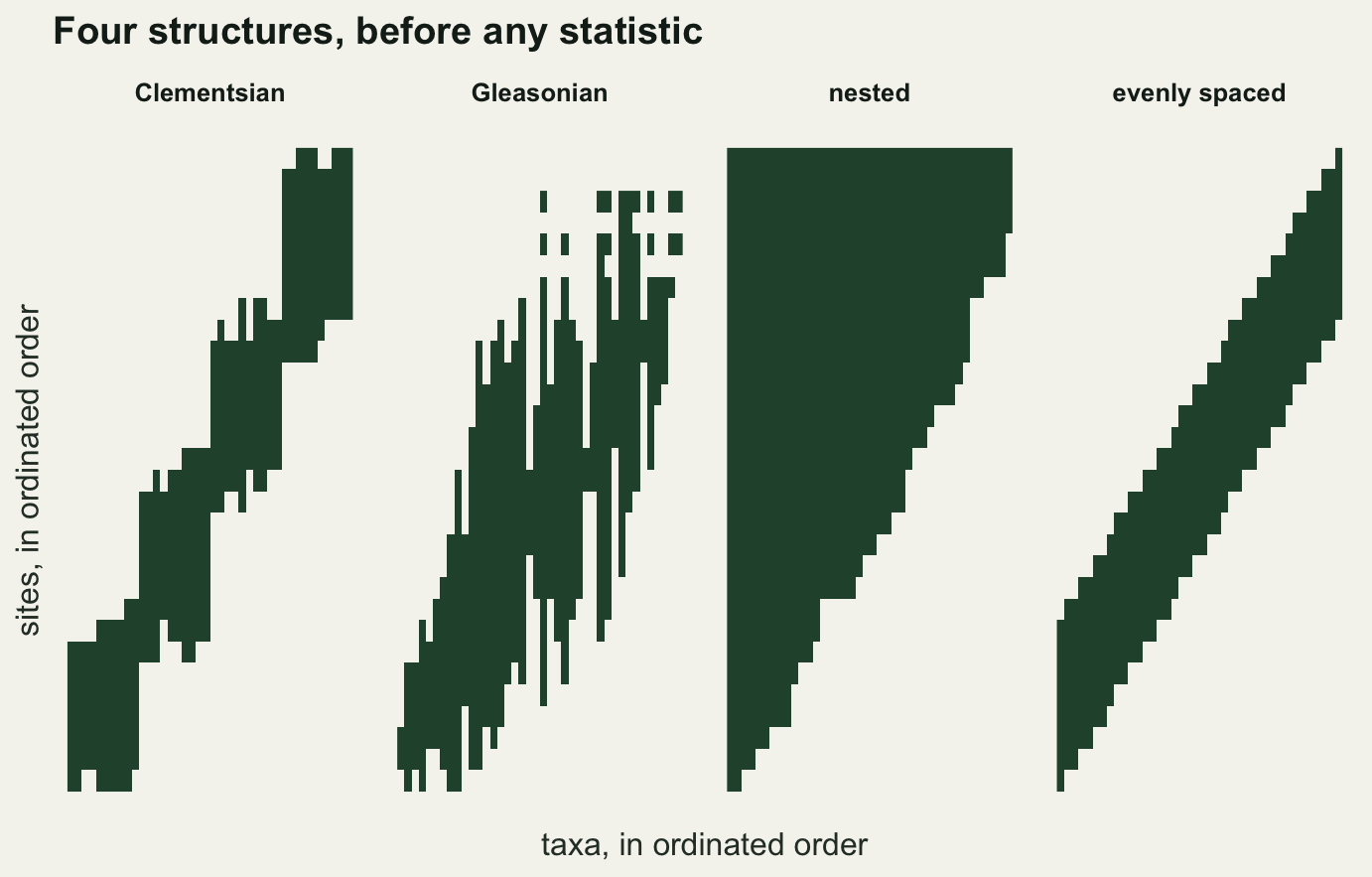
Each generator writes a contiguous range for every taxon along the thirty sites and differs only in where the ranges are put. The Clementsian version puts them in four blocks with shared edges, jittered by a site either way. The Gleasonian version draws two site numbers at random for each taxon and fills between them, which makes the pooled distribution of range boundaries exactly uniform across sites. The nested version starts every range at site one and varies its length. The evenly spaced version marches a fixed range length across the gradient in equal steps. The random version abandons ranges altogether and scatters occurrences.
n_site <- 30; n_taxa <- 40

gen_clementsian <- function() {
  mat <- matrix(0L, n_site, n_taxa)
  grp <- rep(1:4, length.out = n_taxa); edges <- c(1, 9, 16, 23, 30)
  for (j in seq_len(n_taxa)) {
    g <- grp[j]
    a <- max(1, edges[g] + sample(-1:1, 1))
    b <- min(n_site, edges[g + 1] + sample(-1:1, 1))
    mat[a:b, j] <- 1L
  }
  mat
}
gen_gleasonian <- function() {
  mat <- matrix(0L, n_site, n_taxa)
  for (j in seq_len(n_taxa)) {
    bnd <- sample.int(n_site, 2); mat[min(bnd):max(bnd), j] <- 1L
  }
  mat
}
gen_nested <- function() {
  mat <- matrix(0L, n_site, n_taxa)
  len <- sort(sample(4:n_site, n_taxa, replace = TRUE))
  for (j in seq_len(n_taxa)) mat[1:len[j], j] <- 1L
  mat
}
gen_evenly <- function() {
  mat <- matrix(0L, n_site, n_taxa)
  st <- round(seq(1, n_site - 7, length.out = n_taxa))
  for (j in seq_len(n_taxa)) mat[st[j]:min(n_site, st[j] + 7), j] <- 1L
  mat
}
gen_random <- function() {
  mat <- matrix(0L, n_site, n_taxa)
  k <- sample(6:20, n_taxa, replace = TRUE)
  for (j in seq_len(n_taxa)) mat[sample(n_site, k[j]), j] <- 1L
  mat
}

gens <- list(Clementsian = gen_clementsian, Gleasonian = gen_gleasonian,
             nested = gen_nested, "evenly spaced" = gen_evenly, random = gen_random)
set.seed(6120)
example <- gen_clementsian()
ex_ems <- ems(example)
round(ex_ems, 3)
z_coh p_coh z_turn p_turn index p_bc
25.929 0.000 8.834 0.000 2.468 0.000 On one Clementsian matrix the coherence score is 25.9 standard deviations on the coherent side of its null, so there is a gradient. Turnover is 8.8 standard deviations on the high side of its own null, and Morisita’s index is 2.47, comfortably above one. The key returns Clementsian, which is the truth.
Twenty replicate matrices of each type, each tested against one hundred and ninety nine null matrices, give the recovery table.
recover <- function(fun, seed, nrep = 20) {
  set.seed(seed)
  table(replicate(nrep, classify(ems(fun()))))
}
seeds <- c(7101, 7102, 7103, 7104, 7105)
rec <- lapply(seq_along(gens), function(i) recover(gens[[i]], seeds[i]))
names(rec) <- names(gens)
labels_all <- sort(unique(unlist(lapply(rec, names))))
rec_tab <- t(sapply(rec, function(z) {
  out <- setNames(integer(length(labels_all)), labels_all)
  out[names(z)] <- as.integer(z); out
}))
rec_tab
Clementsian clumped nested evenly spaced Gleasonian
Clementsian 20 0 0 0
Gleasonian 13 0 0 7
nested 0 20 0 0
evenly spaced 0 0 20 0
random 0 0 0 0
quasi-structure random
Clementsian 0 0
Gleasonian 0 0
nested 0 0
evenly spaced 0 0
random 1 19correct <- sapply(names(gens), function(nm) {
hit <- if (nm == "nested") grep("nested", colnames(rec_tab), value = TRUE) else nm
sum(rec_tab[nm, intersect(hit, colnames(rec_tab))])
})
correct Clementsian Gleasonian nested evenly spaced random
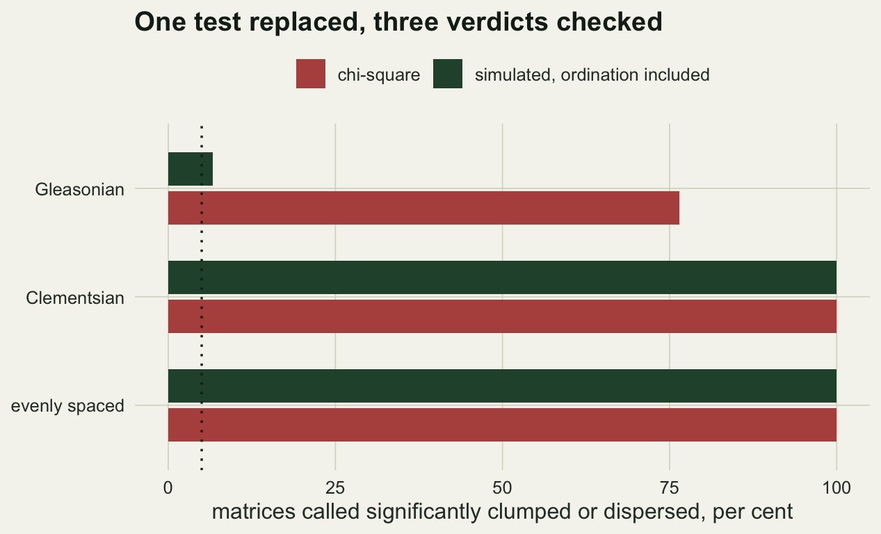
20 7 20 20 19 Clementsian is recovered 20 times out of twenty, nested 20 times, evenly spaced 20 times and random 19 times. Gleasonian is recovered 7 times, and the rest of that row is 13 Clementsian calls.
That is the one failure in the table, and it goes in the worst direction. Independently placed ranges, generated with a boundary distribution that is uniform by construction, are handed back as the structure that implies shared range limits.
Which of the three statistics is wrong
Coherence and turnover are not at fault. Both call the Gleasonian matrices correctly: coherent, with more turnover than the null. The verdict is decided at the last step, by Morisita’s index and its chi-square test.
Morisita’s index is computed on the ordinated matrix, but the chi-square test that judges it knows nothing about the ordination. It treats the boundaries as an allocation of items to sites and asks whether that allocation is more uneven than chance. The ordination has already moved the sites around, and the two questions are not the same. Measuring the index in the true gradient order and again after reciprocal averaging separates them.
set.seed(6140)
eff <- t(replicate(200, {
  mat <- gen_gleasonian()
  c(true_order = morisita(mat), ca_order = morisita(ordinate(mat)))
}))
c(I_true  = mean(eff[, "true_order.index"]),
  rej_true = mean(eff[, "true_order.p"] < 0.05),
  I_ca    = mean(eff[, "ca_order.index"]),
  rej_ca  = mean(eff[, "ca_order.p"] < 0.05))
I_true rej_true I_ca rej_ca
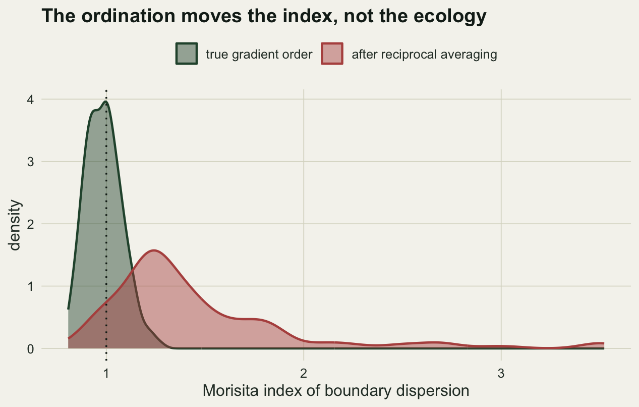
0.9867247 0.0900000 1.4526899 0.7650000 In the true site order the mean index is 0.987, which is what independence should give, and the chi-square test rejects in 9.0 per cent of matrices against a nominal five. After reciprocal averaging the same matrices give a mean index of 1.453 and a rejection rate of 76.5 per cent.
The ordination is not scrambling the sites. Its ordering agrees with the true gradient almost exactly.
set.seed(6141)
fid <- replicate(30, {
  o <- ca_order(gen_gleasonian())
  abs(cor(o$sites, seq_along(o$sites), method = "spearman"))
})
c(mean_rho = mean(fid), min_rho = min(fid))
mean_rho min_rho
0.9616871 0.8177340 Rank correlation between the ordinated order and the true order averages 0.962 and never falls below 0.82. Small local swaps are enough. Reciprocal averaging places sites by their composition, so sites that share several range limits are pulled next to each other, and once they are adjacent the limits they share are counted at neighbouring positions. The clumping is a property of the ordination step, and the chi-square test has no way of knowing that the step happened.
The null model the boundary index actually needs
The obvious repair is to test Morisita’s index against the same null the other two statistics use. It does not work, and the reason is worth seeing. That null holds site richness fixed and scatters occurrences, which destroys range contiguity, so the filled ranges of a null matrix stretch across most of the gradient and their limits pile up at the ends.
set.seed(6150)
mat_g <- gen_gleasonian()
w <- pmax(colSums(mat_g), 1e-9)
bad <- replicate(199, morisita(ordinate(null_matrix(mat_g, w)))[["index"]])
c(observed = morisita(ordinate(mat_g))[["index"]],
  scatter_null_mean = mean(bad))
observed scatter_null_mean
1.101266 2.546239 The observed index is 1.101 and the scattering null averages 2.546. The null is more clumped than the data, so a two sided test against it would announce that these boundaries are unusually evenly spaced.
What the index needs is a null that keeps every range contiguous, keeps the observed range lengths, places the ranges at random along the gradient, and then goes through the same ordination the data went through.
range_null <- function(ord) {
  filled <- fill_ranges(ord); n <- nrow(filled)
  apply(filled, 2, function(v) {
    len <- sum(v); out <- integer(n)
    if (len > 0 && len < n) {
      a <- sample.int(n - len + 1, 1); out[a:(a + len - 1)] <- 1L
    } else out[] <- v
    out
  })
}

bc_simulated <- function(mat, nsim = 199) {
  ord <- ordinate(mat); obs <- morisita(ord)[["index"]]
  sims <- replicate(nsim, morisita(ordinate(range_null(ord)))[["index"]])
  u <- (1 + sum(sims >= obs)) / (1 + nsim)
  c(index = obs, null_mean = mean(sims), p = 2 * min(u, 1 - u))
}

bc_rates <- function(fun, seed, nrep = 30) {
  set.seed(seed)
  out <- t(replicate(nrep, bc_simulated(fun())))
  c(index = mean(out[, "index"]), null_mean = mean(out[, "null_mean"]),
    reject = 100 * mean(out[, "p"] < 0.05))
}
repair <- rbind(Gleasonian    = bc_rates(gen_gleasonian, 6161),
                Clementsian   = bc_rates(gen_clementsian, 6162),
                `evenly spaced` = bc_rates(gen_evenly, 6163))
round(repair, 3)
index null_mean reject
Gleasonian 1.550 1.819 6.667
Clementsian 2.418 1.068 100.000
evenly spaced 0.778 1.077 100.000On Gleasonian matrices the simulated test rejects in 6.7 per cent of cases, against the 76.5 per cent of the chi-square version. The null mean is 1.819, which reproduces the inflation the ordination causes instead of ignoring it. Power is intact: Clementsian matrices are still called clumped in 100 per cent of cases and evenly spaced matrices are still called dispersed in 100 per cent.
What to report
Report the three statistics separately and say how each was tested. A metacommunity type is a conclusion assembled from three tests with different properties, and collapsing them into one word hides the fact that the last of the three is the one that chose the name.
If the label matters to the argument, run the boundary index against a null that preserves range contiguity and repeats the ordination, and report that p value rather than the chi-square one. Thirty lines of code separate a 76 per cent false positive rate from a 7 per cent one, and neither the software nor the published key will tell you which one you are quoting.
Distinguish coherence from the other two in the writing as well. Coherence is the precondition: without it there is no gradient and the remaining statistics describe a matrix that has no ordering to describe. Turnover and boundary clumping are the ones that separate the named types, and only one of them names them.
Honest limits
The statistics here follow the published definitions, but they are written from scratch rather than taken from the metacom package, which is the standard implementation. The turnover count uses the range perspective, which fills embedded absences before counting replacements, and the boundary index counts the first and last occupied site of each filled range. An implementation that treats ties, empty rows or single site ranges differently will produce different numbers on the same data, so the rates here are not transferable constants.
Everything runs on thirty sites and forty taxa. The chi-square approximation behind Morisita’s index degrades when boundaries are few relative to sites, and the inflation measured here will change with the shape of the matrix. The direction is the part that carries over: the ordination concentrates boundaries, so the chi-square test is anticonservative, not conservative.
The generators are noise free. Every occurrence in these matrices is real and every absence is a true absence. Imperfect detection puts zeros inside occupied ranges, which is exactly what the coherence statistic counts, so a survey with a detection probability well below one will push real structure towards the random verdict for a reason that has nothing to do with the metacommunity.
Finally, the repair fixes calibration, not interpretation. A matrix that passes the corrected test still only shows that range limits coincide more than a randomly placed set of ranges of the same lengths would. Coincident limits are compatible with shared environmental thresholds, with competition, and with a sampling design whose sites happen to straddle one abrupt habitat edge.
References
Leibold MA, Mikkelson GM 2002 Oikos 97(2):237-250 (10.1034/j.1600-0706.2002.970210.x)
Presley SJ, Higgins CL, Willig MR 2010 Oikos 119(6):908-917 (10.1111/j.1600-0706.2010.18544.x)
Morisita M 1962 Population Ecology 4(1):1-7 (10.1007/BF02533903)
Hill MO 1973 Journal of Ecology 61(1):237-249 (10.2307/2258931)
Dallas T 2014 Ecography 37(4):402-405 (10.1111/j.1600-0587.2013.00695.x)