library(ggplot2)

te_pal <- list(forest = "#275139", green = "#2f8f63", sage = "#93a87f",
               clay = "#b5534e", gold = "#cda23f", line = "#dad9ca",
               ink = "#16241d", paper = "#f5f4ee")

fmt <- function(x, digits = 4) formatC(x, format = "f", digits = digits)

theme_te <- function() {
  theme_minimal(base_size = 12) +
    theme(panel.grid.minor = element_blank(),
          panel.grid.major = element_line(colour = "#e7e6dc"),
          plot.background = element_rect(fill = "#f5f4ee", colour = NA),
          panel.background = element_rect(fill = "#f5f4ee", colour = NA),
          plot.title = element_text(face = "bold", colour = te_pal$ink),
          axis.title = element_text(colour = "#2c3a31"),
          legend.position = "bottom")
}How many components in a mixture?
R
mixture models
model selection
ecology tutorial
Choosing the number of components in a mixture model in R: why the likelihood ratio test fails, and what the bootstrap, BIC and ICL each recover instead.
The perch came out of the gill nets over four mornings in late August, and by the end of the week the notebook held a few hundred standard lengths. Somebody drew the histogram on the whiteboard in the field station kitchen, and the shape had a shoulder: a tall pile of small fish, then a lump further right that was too heavy to be a tail. The obvious reading was two age classes, the young of the year and everything older, and the obvious next step was to fit a two-component mixture and report the two mean lengths.
The awkward part was the sentence that had to go under the figure. Not “here are the two means”, which the fitter will happily produce, but “there are two age classes in this lake”. That second sentence is a claim about the number of components, and it is the one part of a mixture analysis where the usual machinery quietly stops working. Fit two components and you get two means. Fit three and you get three. The fitter never refuses.
The test everybody reaches for is the likelihood ratio: fit k components, fit k plus one, take twice the difference in log-likelihood, look it up in a chi-squared table. That test is not valid here, and the reason is structural rather than a matter of sample size. Under the null that k components suffice, the extra component has to have either zero weight, which sits on the boundary of the parameter space, or a mean equal to one of the existing means, which leaves its own mean unidentified. Both of those break the conditions the chi-squared limit needs.
This post measures the damage rather than asserting it, and then measures three things that do work: a parametric bootstrap version of the same test, the information criteria (AIC, BIC and ICL), and the separation between components that has to be there before any of it has a chance. Every simulation below prints the replicate count it ran on, and the whole post fits in base R plus ggplot2, with the EM algorithm written out in about twenty lines.
The fitting machinery itself is built and explained in fitting a mixture of normals in R; this post rebuilds a compact version so it stands alone, but that one is the place to go if the EM steps are new. The question of whether the second component is real at all, as opposed to skewness in one population, is taken further in when a mixture is really skewness.
The fitter, written out once
Everything below leans on one function, so it belongs on the page. em_mix fits a k-component univariate normal mixture by expectation maximisation. The E step computes the posterior probability that each observation came from each component; the M step sets the weights, means and standard deviations to their weighted averages. Two options matter later: equal_var decides whether the components share one standard deviation, and starts decides how many initialisations are tried before the best fit is kept.
Two guards are in there for reasons that come up in the last section. The standard deviations are floored at five per cent of the sample standard deviation, because with unequal variances the likelihood is unbounded: a component can sit on a single point, shrink its variance towards zero and send the likelihood to infinity. And the iteration count is capped, because near the null the algorithm crawls, and an uncapped run would spend most of the post’s budget in cases where the answer barely moves.
em_mix <- function(x, k, equal_var = TRUE, max_iter = 60, tol = 1e-6, starts = 1) {
  n <- length(x)
  sx <- sqrt(sum((x - mean(x))^2) / n)
  fl <- 0.05 * sx
  best <- NULL
  best_ll <- -Inf
  dens <- matrix(0, n, k)
  for (s in seq_len(starts)) {
    mu <- if (s == 1) as.numeric(quantile(x, (seq_len(k) - 0.5) / k)) else x[sample.int(n, k)]
    sg <- rep(sx, k)
    w <- rep(1 / k, k)
    ll <- -Inf
    ll_old <- -Inf
    for (it in seq_len(max_iter)) {
      for (j in seq_len(k)) dens[, j] <- w[j] * dnorm(x, mu[j], sg[j])
      tot <- .rowSums(dens, n, k) + 1e-300
      ll <- sum(log(tot))
      resp <- dens / tot
      nk <- .colSums(resp, n, k) + 1e-12
      w <- nk / n
      mu <- .colSums(resp * x, n, k) / nk
      ss <- numeric(k)
      for (j in seq_len(k)) ss[j] <- sum(resp[, j] * (x - mu[j])^2)
      sg <- if (equal_var) rep(sqrt(sum(ss) / n), k) else sqrt(ss / nk)
      sg <- pmax(sg, fl)
      if (abs(ll - ll_old) < tol * (abs(ll_old) + 1)) break
      ll_old <- ll
    }
    if (ll > best_ll) {
      best_ll <- ll
      best <- list(w = w, mu = mu, sg = sg, ll = ll, resp = resp, iter = it)
    }
  }
  best$k <- k
  best$npar <- if (equal_var) 2 * k else 3 * k - 1
  best
}

fit_one <- function(x) {
  n <- length(x)
  m <- mean(x)
  s <- sqrt(sum((x - m)^2) / n)
  list(w = 1, mu = m, sg = s, ll = sum(dnorm(x, m, s, log = TRUE)),
       resp = matrix(1, n, 1), k = 1, npar = 2)
}

crit_all <- function(f, n) {
  p <- pmax(f$resp, 1e-12)
  ent <- -sum(ifelse(f$resp > 1e-12, f$resp * log(p), 0))
  c(aic = -2 * f$ll + 2 * f$npar,
    bic = -2 * f$ll + f$npar * log(n),
    icl = -2 * f$ll + f$npar * log(n) + 2 * ent,
    ent = ent)
}

r_mix <- function(n, w, mu, sg) {
  z <- sample.int(length(w), n, TRUE, prob = w)
  rnorm(n, mu[z], sg[z])
}set.seed(20260729)
chk_n <- 600
chk_x <- r_mix(chk_n, c(0.35, 0.65), c(0, 4), c(1, 1))
chk_f <- em_mix(chk_x, 2, max_iter = 200, starts = 3)
print(c(n = chk_n)) n
600 print(round(c(w1_true = 0.35, w1_hat = min(chk_f$w),
mu1_true = 0, mu1_hat = min(chk_f$mu),
mu2_true = 4, mu2_hat = max(chk_f$mu),
sigma_true = 1, sigma_hat = chk_f$sg[1]), 4)) w1_true w1_hat mu1_true mu1_hat mu2_true mu2_hat sigma_true
0.3500 0.3314 0.0000 0.0867 4.0000 3.9927 1.0000
sigma_hat
1.0177 chk_c <- crit_all(chk_f, chk_n)
print(round(chk_c, 3)) aic bic icl ent
2417.167 2434.755 2511.528 38.387 print(round(c(icl_minus_bic = chk_c[["icl"]] - chk_c[["bic"]]), 3))icl_minus_bic
76.773 With 600 observations from a known mixture, the fitter returns a smaller weight of 0.3314 against a true 0.3500, means of 0.0867 and 3.9927 against true values of 0.0000 and 4.0000, and a common standard deviation of 1.0177 against a true 1.0000. Nothing surprising: given the number of components, estimating the components is easy.
crit_all returns the three selection criteria on the deviance scale, so smaller is better in all three. AIC penalises each parameter by two, BIC by log(n), and ICL takes BIC and adds twice the entropy of the classification. That entropy term is the sum over observations and components of the posterior probability times its own logarithm, negated; it is zero when every observation belongs unambiguously to one component and large when the posteriors sit near one half. For a one-component fit it is exactly zero, so ICL and BIC agree there by construction. For the fit above the entropy is 38.387, which puts ICL 76.773 above BIC on a BIC of 2434.755. Small on that scale, but not nothing, and two sections below are about the cases where it decides the answer.
The test that does not work, measured
Take the simplest possible null: the data really do come from one normal component. Simulate a few hundred such data sets, fit one and two components to each, and record twice the difference in log-likelihood. If the chi-squared approximation held, that statistic would follow a chi-squared distribution, and the only question would be the degrees of freedom.
That question already has no clean answer. Counting parameters, the equal-variance one-component model has two (a mean and a variance) and the two-component model has four (two means, one variance, one weight), so the difference is two. An analyst who reasons that the weight is stuck on the boundary and therefore should not count arrives at one. An analyst working in the unequal-variance family counts three. All three numbers appear in real analyses, so the honest thing is to check all three against the same simulated null.
set.seed(20260729)
rep_a <- 300
n_a <- 200
lr_a <- numeric(rep_a)
for (r in seq_len(rep_a)) {
  x <- rnorm(n_a)
  lr_a[r] <- 2 * (em_mix(x, 2, max_iter = 80, starts = 2)$ll - fit_one(x)$ll)
}
qs <- c(0.5, 0.9, 0.95, 0.99)
print(c(replicates = rep_a, n = n_a, em_max_iter = 80, em_starts = 2))
replicates n em_max_iter em_starts
300 200 80 2 print(round(rbind(empirical = quantile(lr_a, qs),
chisq_df1 = qchisq(qs, 1),
chisq_df2 = qchisq(qs, 2),
chisq_df3 = qchisq(qs, 3)), 3)) 50% 90% 95% 99%
empirical 0.776 4.171 5.706 8.818
chisq_df1 0.455 2.706 3.841 6.635
chisq_df2 1.386 4.605 5.991 9.210
chisq_df3 2.366 6.251 7.815 11.345print(c(collapse_threshold = 0.01))collapse_threshold
0.01 print(round(c(mean_stat = mean(lr_a),
prop_below_0.01 = mean(lr_a < 0.01),
fpr_df1 = mean(lr_a > qchisq(0.95, 1)),
fpr_df2 = mean(lr_a > qchisq(0.95, 2)),
fpr_df3 = mean(lr_a > qchisq(0.95, 3))), 4)) mean_stat prop_below_0.01 fpr_df1 fpr_df2 fpr_df3
1.5224 0.1633 0.1167 0.0467 0.0267 The result is more interesting than a flat failure. At the 95th percentile the empirical statistic reaches 5.706, and the chi-squared quantiles for one, two and three degrees of freedom are 3.841, 5.991 and 7.815. So the false positive rate at a nominal five per cent comes out at 0.1167 with one degree of freedom, 0.0467 with two, and 0.0267 with three. The middle choice, which is also the naive parameter count, is close to nominal. The boundary argument that sounds most careful is the one that inflates the error rate to more than twice its nominal value.
Look at the median and the picture changes completely. The empirical median is 0.776 against 1.386 for chi-squared on two degrees of freedom, and 0.1633 of the replicates produced a statistic below 0.01, meaning the two-component fit collapsed onto the one-component one and bought nothing at all. A chi-squared distribution has no such spike at zero. The empirical distribution is a point mass at the origin glued to a right tail, and only the tail happens to line up with a chi-squared curve.
That coincidence is the trap. Nothing in the simulation says it will survive a change of sample size, of family, or of the null value of k. So repeat the whole exercise one level up: generate from a genuine two-component mixture with means 0 and 3 and equal weights, then test two components against three.
set.seed(20260730)
rep_b <- 150
n_b <- 250
lr_b <- numeric(rep_b)
for (r in seq_len(rep_b)) {
  x <- r_mix(n_b, c(0.5, 0.5), c(0, 3), c(1, 1))
  lr_b[r] <- 2 * (em_mix(x, 3, max_iter = 80, starts = 2)$ll -
                    em_mix(x, 2, max_iter = 80, starts = 2)$ll)
}
print(c(replicates = rep_b, n = n_b))
replicates n
150 250 print(round(rbind(empirical = quantile(lr_b, qs), chisq_df2 = qchisq(qs, 2)), 3)) 50% 90% 95% 99%
empirical 0.493 4.136 5.308 8.958
chisq_df2 1.386 4.605 5.991 9.210print(round(c(prop_below_0.01 = mean(lr_b < 0.01),
fpr_df1 = mean(lr_b > qchisq(0.95, 1)),
fpr_df2 = mean(lr_b > qchisq(0.95, 2)),
fpr_df3 = mean(lr_b > qchisq(0.95, 3))), 4))prop_below_0.01 fpr_df1 fpr_df2 fpr_df3
0.3067 0.1133 0.0333 0.0267 qgrid <- seq(0, 12, length.out = 241)
ecdf_a <- ecdf(lr_a)
ecdf_b <- ecdf(lr_b)
null_df <- rbind(
data.frame(q = qgrid, p = ecdf_a(qgrid), series = "simulated",
panel = "one component tested against two"),
data.frame(q = qgrid, p = pchisq(qgrid, 1), series = "chi-squared, df = 1",
panel = "one component tested against two"),
data.frame(q = qgrid, p = pchisq(qgrid, 2), series = "chi-squared, df = 2",
panel = "one component tested against two"),
data.frame(q = qgrid, p = pchisq(qgrid, 3), series = "chi-squared, df = 3",
panel = "one component tested against two"),
data.frame(q = qgrid, p = ecdf_b(qgrid), series = "simulated",
panel = "two components tested against three"),
data.frame(q = qgrid, p = pchisq(qgrid, 1), series = "chi-squared, df = 1",
panel = "two components tested against three"),
data.frame(q = qgrid, p = pchisq(qgrid, 2), series = "chi-squared, df = 2",
panel = "two components tested against three"),
data.frame(q = qgrid, p = pchisq(qgrid, 3), series = "chi-squared, df = 3",
panel = "two components tested against three"))
null_df$series <- factor(null_df$series,
levels = c("simulated", "chi-squared, df = 1",
"chi-squared, df = 2", "chi-squared, df = 3"))
ggplot(null_df, aes(q, p, colour = series, linewidth = series)) +
geom_line() +
facet_wrap(~ panel) +
scale_colour_manual(values = c(te_pal$ink, te_pal$clay, te_pal$gold, te_pal$green),
name = NULL) +
scale_linewidth_manual(values = c(1.4, 0.7, 0.7, 0.7), guide = "none") +
scale_x_continuous(breaks = c(0, 2.5, 5, 7.5, 10)) +
labs(title = "The null distribution is not chi-squared",
x = "likelihood ratio statistic", y = "probability at or below") +
theme_te() +
theme(panel.spacing.x = grid::unit(14, "pt"),
plot.margin = margin(6, 12, 6, 6))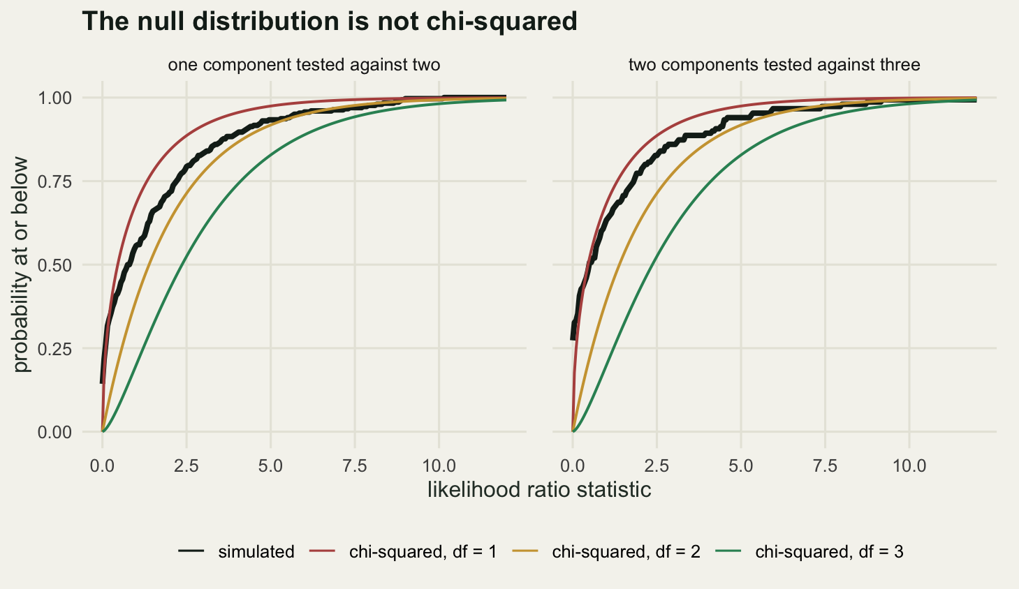
At the second level the point mass at zero has grown to 0.3067 of replicates, up from 0.1633, and the false positive rate on two degrees of freedom has moved to 0.0333 from 0.0467. The one degree of freedom rate stays high at 0.1133. So the reference that looked calibrated in the first setting has drifted in the second, in a direction nobody could have predicted from the first, and the choice that looked most conservative in theory is wrong by a factor of about two in both.
The figure shows why summarising this with a single false positive rate hides the problem. Both simulated curves leave the vertical axis at a positive height, because a sizeable share of data sets give a two-component fit that is numerically identical to the one-component fit. Then they climb steeply, are overtaken by the one degree of freedom reference almost at once, and run above both the two and three degree of freedom curves through the middle of the range. There is no degrees of freedom setting that matches the whole curve. Picking one is picking which part of the distribution to get right, and the part a test needs is the part nobody checks.
The bootstrap version, and what it costs
The repair is old and simple. If you do not know the null distribution of the statistic, simulate it. Fit the k-component model to the real data, treat the fitted model as the truth, generate many data sets from it, refit both the k and the k plus one component models to each, and see where the observed statistic falls in that pile. The p-value is the rank of the observed statistic among the simulated ones, with the observed value counted in the numerator and denominator so the test stays valid at small numbers of replicates.
boot_lrt <- function(x, boot_b) {
  f1 <- fit_one(x)
  stat_obs <- 2 * (em_mix(x, 2, max_iter = 35)$ll - f1$ll)
  n <- length(x)
  stat_b <- numeric(boot_b)
  for (b in seq_len(boot_b)) {
    xb <- rnorm(n, f1$mu, f1$sg)
    stat_b[b] <- 2 * (em_mix(xb, 2, max_iter = 35)$ll - fit_one(xb)$ll)
  }
  c(stat = stat_obs, p = (1 + sum(stat_b >= stat_obs)) / (boot_b + 1))
}

set.seed(20260805)
n_sets <- 60
boot_b <- 99
n_c <- 60
res_boot <- t(sapply(seq_len(n_sets), function(s) boot_lrt(rnorm(n_c), boot_b)))
p_boot <- res_boot[, "p"]
p_naive1 <- pchisq(res_boot[, "stat"], 1, lower.tail = FALSE)
p_naive2 <- pchisq(res_boot[, "stat"], 2, lower.tail = FALSE)
print(c(null_data_sets = n_sets, bootstrap_replicates = boot_b, n = n_c,
        em_fits = n_sets * (boot_b + 1)))
null_data_sets bootstrap_replicates n
60 99 60
em_fits
6000 print(round(c(size_boot_05 = mean(p_boot <= 0.05),
size_boot_10 = mean(p_boot <= 0.10),
size_boot_20 = mean(p_boot <= 0.20),
size_naive_df1_05 = mean(p_naive1 <= 0.05),
size_naive_df2_05 = mean(p_naive2 <= 0.05),
mean_p_boot = mean(p_boot), uniform_mean_p = 0.5,
mc_se_of_size = sqrt(0.05 * 0.95 / n_sets)), 4)) size_boot_05 size_boot_10 size_boot_20 size_naive_df1_05
0.0667 0.0833 0.1333 0.1000
size_naive_df2_05 mean_p_boot uniform_mean_p mc_se_of_size
0.0333 0.5553 0.5000 0.0281 Across 60 null data sets of 60 observations each, the bootstrap test rejects at the five per cent level in 0.0667 of them, at the ten per cent level in 0.0833, and at the twenty per cent level in 0.1333. The Monte Carlo standard error on the first of those, with 60 data sets, is 0.0281, so all three sit within sampling noise of their nominal levels. The mean bootstrap p-value is 0.5553, against 0.5000 for a perfectly uniform p-value. On the same data sets the naive test on one degree of freedom rejects 0.1000 of the time and the two degree of freedom version 0.0333.
lev <- seq(0.01, 0.99, by = 0.01)
size_df <- rbind(
  data.frame(level = lev, rate = sapply(lev, function(a) mean(p_boot <= a)),
             series = "bootstrap"),
  data.frame(level = lev, rate = sapply(lev, function(a) mean(p_naive1 <= a)),
             series = "chi-squared, df = 1"),
  data.frame(level = lev, rate = sapply(lev, function(a) mean(p_naive2 <= a)),
             series = "chi-squared, df = 2"))

ggplot(size_df, aes(level, rate, colour = series)) +
  geom_abline(intercept = 0, slope = 1, linetype = "dashed",
              colour = te_pal$ink, linewidth = 0.5) +
  geom_step(linewidth = 1) +
  scale_colour_manual(values = c(te_pal$forest, te_pal$clay, te_pal$gold),
                      name = NULL) +
  labs(title = "Calibration of three tests on the same null data",
       x = "nominal level", y = "measured rejection rate") +
  theme_te()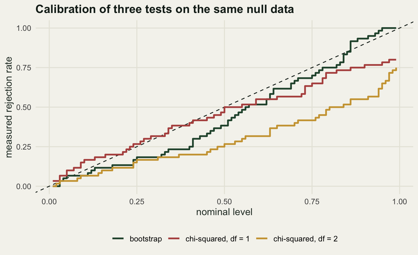
The figure shows where each curve pays. The bootstrap sits on the diagonal at the left edge, to within Monte Carlo error, and that is the part that matters, because a test is used at a small level and the calibration there is the calibration you spend; it then sags below the diagonal through the middle of the range, so it is mildly conservative at levels nobody reports. The one degree of freedom curve does the opposite, and in the more expensive direction: over the whole left half of the range it rejects more often than it promises.
The price is arithmetic. Each bootstrap test above cost 100 EM fits of the two-component model, one for the observed data and 99 for the simulated nulls, and measuring the size of the test took 6000 fits in total. The one-component fits are free because the normal maximum likelihood estimates are closed form. Against a single chi-squared lookup, that is a factor of 100.
How many replicates does the test actually need? The smallest attainable p-value is one over the number of replicates plus one, so the count sets a floor on what the test can report, and it also sets the exact size of the test at a given level.
b_grid <- c(9, 19, 49, 99, 399, 1999)
print(data.frame(B = b_grid,
                 smallest_p = round(1 / (b_grid + 1), 4),
                 exact_size_at_05 = round(floor(0.05 * (b_grid + 1)) / (b_grid + 1), 4),
                 mc_se_at_p_05 = round(sqrt(0.05 * 0.95 / b_grid), 4),
                 em_fits_per_test = b_grid + 1))
B smallest_p exact_size_at_05 mc_se_at_p_05 em_fits_per_test
1 9 0.1000 0.00 0.0726 10
2 19 0.0500 0.05 0.0500 20
3 49 0.0200 0.04 0.0311 50
4 99 0.0100 0.05 0.0219 100
5 399 0.0025 0.05 0.0109 400
6 1999 0.0005 0.05 0.0049 2000With 9 replicates the smallest reportable p-value is 0.1000 and the exact size of a five per cent test is 0.00: the test can never reject, whatever the data say. With 49 replicates the size is 0.04 rather than 0.0500, because the achievable p-values step in units of 0.0200 and none of them lands on the nominal level. 99 replicates is the smallest count that gives exactly 0.05 while still allowing a p-value low enough to be worth quoting, and its Monte Carlo standard error near p equal to 0.0500 is 0.0219. If the reported p-value has to separate 0.0200 from 0.0500, that error has to come down, and it only comes down as the square root: 399 replicates gives 0.0109 and 1999 gives 0.0049.
So the practical recommendation is 99 replicates for a decision at the five per cent level, and 399 or more if the p-value itself is going into the paper. Multiply by the cost of the EM fits and by the number of values of k under consideration, and a full model selection over one to four components is several thousand fits. That is minutes rather than seconds, and it is why the information criteria stay popular.
AIC, BIC and the entropy penalty
The criteria cost one fit each and no simulation. All three are on the deviance scale here, so the smallest value wins. The comparison worth making is not which formula is prettiest but how often each one lands on the number of components that generated the data. Run six cells: one true component; two true components at separations of two, three and five standard deviations; three true components at separations of three and five. Fit one to four components in the equal-variance family and record what each criterion picks.
gen_cell <- function(kt, d, n) {
  if (kt == 1) rnorm(n) else r_mix(n, rep(1 / kt, kt), (seq_len(kt) - 1) * d, rep(1, kt))
}

cells <- list(c(1, 0), c(2, 2), c(2, 3), c(2, 5), c(3, 3), c(3, 5))
rep_c <- 60
n_d <- 250
set.seed(20260802)
grid_c <- NULL
for (cl in cells) {
  kt <- cl[1]
  d <- cl[2]
  sel <- matrix(0L, rep_c, 3)
  for (r in seq_len(rep_c)) {
    x <- gen_cell(kt, d, n_d)
    cm <- rbind(crit_all(fit_one(x), n_d),
                crit_all(em_mix(x, 2, max_iter = 50), n_d),
                crit_all(em_mix(x, 3, max_iter = 50, starts = 2), n_d),
                crit_all(em_mix(x, 4, max_iter = 50, starts = 2), n_d))
    sel[r, ] <- apply(cm[, 1:3], 2, which.min)
  }
  grid_c <- rbind(grid_c, data.frame(
    k_true = kt, delta = d,
    aic = mean(sel[, 1] == kt), bic = mean(sel[, 2] == kt), icl = mean(sel[, 3] == kt),
    aic_over = mean(sel[, 1] > kt), bic_over = mean(sel[, 2] > kt),
    icl_over = mean(sel[, 3] > kt),
    bic_under = mean(sel[, 2] < kt), icl_under = mean(sel[, 3] < kt)))
}
print(c(replicates_per_cell = rep_c, n = n_d, candidate_k_min = 1, candidate_k_max = 4))
replicates_per_cell n candidate_k_min candidate_k_max
60 250 1 4 print(round(grid_c, 3)) k_true delta aic bic icl aic_over bic_over icl_over bic_under icl_under
1 1 0 0.900 1.000 1 0.100 0.000 0 0.000 0
2 2 2 0.617 0.117 0 0.017 0.000 0 0.883 1
3 2 3 0.850 1.000 0 0.150 0.000 0 0.000 1
4 2 5 0.933 1.000 1 0.067 0.000 0 0.000 0
5 3 3 1.000 0.833 0 0.000 0.000 0 0.167 1
6 3 5 0.933 0.983 1 0.067 0.017 0 0.000 0print(round(colMeans(grid_c[, 3:10]), 4)) aic bic icl aic_over bic_over icl_over bic_under icl_under
0.8722 0.8222 0.5000 0.0667 0.0028 0.0000 0.1750 0.5000 lab_c <- ifelse(grid_c$k_true == 1, "k = 1",
paste0("k = ", grid_c$k_true, ", sep ", grid_c$delta))
crit_df <- rbind(
data.frame(cell = lab_c, rate = grid_c$aic, series = "AIC"),
data.frame(cell = lab_c, rate = grid_c$bic, series = "BIC"),
data.frame(cell = lab_c, rate = grid_c$icl, series = "ICL"))
crit_df$cell <- factor(crit_df$cell, levels = lab_c)
zero_df <- crit_df
zero_df$mark <- ifelse(zero_df$rate == 0, "0", "")
zero_df$rate <- 0.012
ggplot(crit_df, aes(cell, rate, fill = series)) +
geom_col(position = position_dodge(width = 0.8), width = 0.72) +
geom_text(data = zero_df, aes(cell, rate, group = series, label = mark),
position = position_dodge(width = 0.8), vjust = 0, size = 3.2,
colour = te_pal$clay, inherit.aes = FALSE) +
scale_fill_manual(values = c(te_pal$green, te_pal$gold, te_pal$clay), name = NULL) +
scale_y_continuous(limits = c(0, 1.02), expand = c(0, 0)) +
labs(title = "How often each criterion recovers the truth",
x = NULL, y = "proportion of replicates correct") +
theme_te() +
theme(plot.margin = margin(6, 14, 6, 6))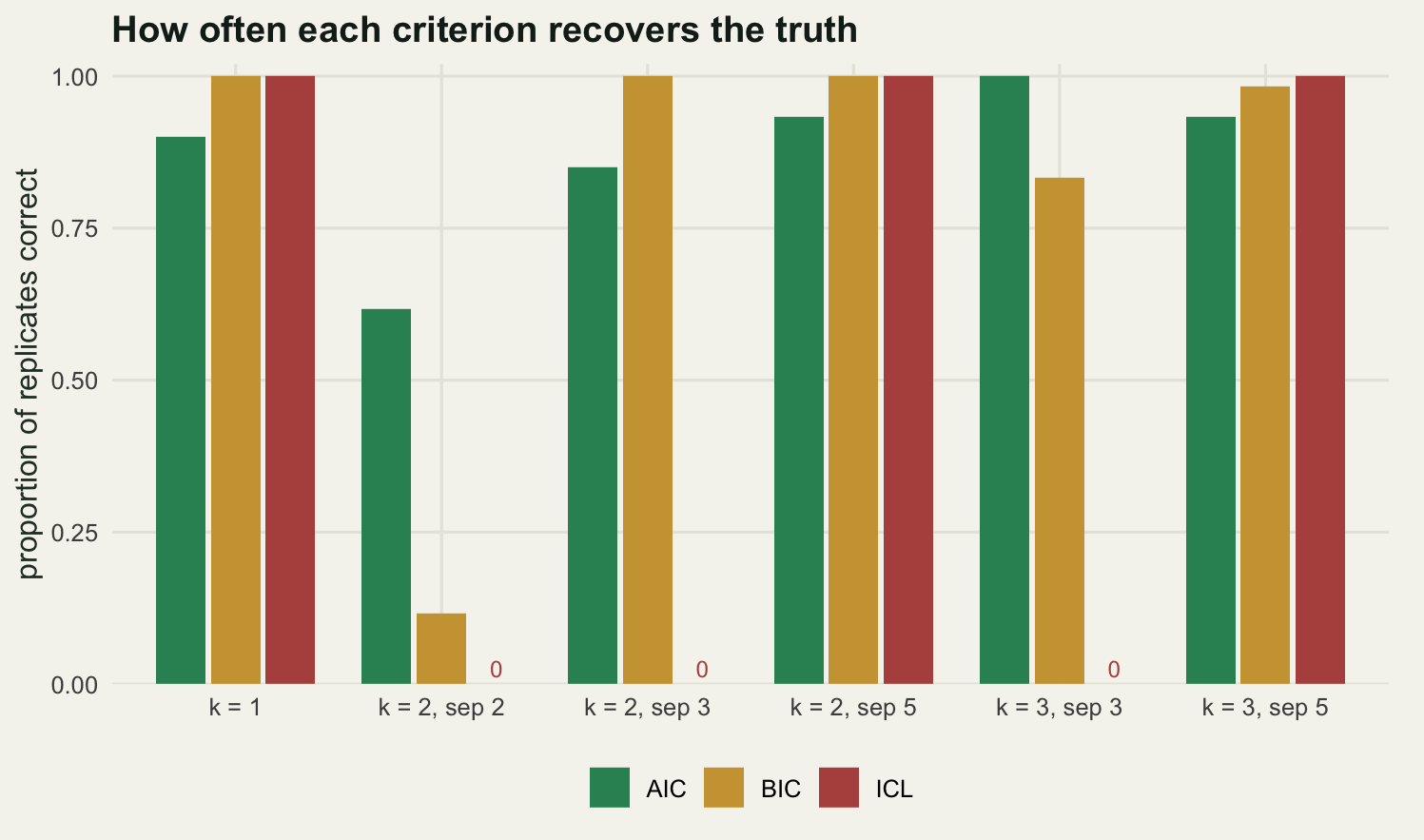
Averaged over the six cells, AIC recovers the truth 0.8722 of the time and BIC 0.8222. That is the wrong way round if the received advice is right, and the row that flips it is the one with two components separated by two standard deviations: AIC gets that cell right 0.617 of the time and BIC 0.117. The received advice is not wrong about the mechanism. AIC does over-select, at an average rate of 0.0667 against BIC’s 0.0028. What the advice leaves out is that BIC’s own error, under-selecting, runs at 0.1750 across the same cells, and in this grid the under-selection costs more than the over-selection does.
Which of those errors you would rather make is not a statistical question. If the second component is a hypothesis to be defended in a paper, BIC’s caution is the right default and AIC’s 0.100 over-selection rate on pure one-component data is exactly the false discovery you do not want. If the mixture is a density estimate feeding into something else, an extra component costs two parameters and improves the fit, and missing a real one is the worse outcome.
ICL is not competing in the same event. Its column in the table is all ones and zeros: it is right in every replicate of the one-component cell and of the two cells where the components are five standard deviations apart, and wrong in every replicate of the three cells where they overlap. Averaged over the grid that is a recovery rate of 0.5000, an under-selection rate of 0.5000 and an over-selection rate of 0.0000. That is not a defect. The entropy term makes ICL ask whether the components can be told apart, not whether the density needs them.
Where BIC and ICL disagree, and who is right
The cleanest disagreement is at a separation of three. Generate two components that far apart with equal weights and a comfortable sample size, fit both models, and record how each criterion votes along with how well the fitted mixture can actually label individuals. The Bayes limit on classification accuracy at separation d, with equal weights and unit variances, is one minus the normal tail below minus d over two, so it is available in closed form to check the fitted classifier against.
set.seed(20260806)
rep_e <- 60
n_e <- 400
dis <- NULL
for (d in c(3, 5)) {
  acc <- ent <- dbic <- dicl <- numeric(rep_e)
  for (r in seq_len(rep_e)) {
    z <- sample.int(2, n_e, TRUE)
    x <- rnorm(n_e, c(0, d)[z], 1)
    c1 <- crit_all(fit_one(x), n_e)
    f2 <- em_mix(x, 2, max_iter = 60, starts = 2)
    c2 <- crit_all(f2, n_e)
    hit <- mean(max.col(f2$resp) == z)
    acc[r] <- max(hit, 1 - hit)
    ent[r] <- c2["ent"]
    dbic[r] <- c1["bic"] - c2["bic"]
    dicl[r] <- c1["icl"] - c2["icl"]
  }
  dis <- rbind(dis, data.frame(
    separation = d, accuracy = mean(acc), bayes_accuracy = 1 - pnorm(-d / 2),
    misassigned = mean(1 - acc) * n_e, entropy = mean(ent),
    bic_gain = mean(dbic), icl_gain = mean(dicl),
    bic_picks_two = sum(dbic > 0), icl_picks_two = sum(dicl > 0)))
}
print(c(replicates = rep_e, n = n_e))
replicates n
60 400 print(round(dis, 3)) separation accuracy bayes_accuracy misassigned entropy bic_gain icl_gain
1 3 0.933 0.933 26.867 66.192 40.251 -92.134
2 5 0.993 0.994 2.700 6.974 243.728 229.780
bic_picks_two icl_picks_two
1 60 0
2 60 60print(round(c(misassigned_sep3 = dis$misassigned[1],
misassigned_sep5 = dis$misassigned[2]), 1))misassigned_sep3 misassigned_sep5
26.9 2.7 At a separation of 3, BIC prefers two components in 60 of the 60 replicates and ICL prefers two in 0 of them. The average BIC gain for the second component is 40.251 in its favour and the average ICL gain is -92.134, which is to say ICL is against by a wide margin. The classification entropy of the two-component fit averages 66.192 over 400 observations, and doubling that is more than enough to swamp the likelihood gain.
Both are right about different things, and the accuracy column says which is which. The fitted two-component model assigns 0.933 of individuals to the correct component, against a Bayes limit of 0.933 for the true parameters. The fit is essentially at the ceiling, and the ceiling still leaves about 26.9 of the 400 fish in the wrong group. If the question is whether the length distribution is a mixture, BIC’s answer is correct and ICL’s is a false negative. If the question is which fish belong to which cohort, ICL is telling you that the answer will be wrong for 26.9 of them however well the mixture is fitted, and that a table of per-individual assignments would be reporting noise as structure.
At a separation of 5 the disagreement vanishes. Accuracy climbs to 0.993 against a Bayes limit of 0.994, entropy falls to 6.974, and both criteria pick two components in all 60 replicates. The rule that comes out of this is short: use BIC when the model is the deliverable and ICL when the labels are.
How much separation, and how many animals
The textbook fact about two equal-weight normal components with a common variance is that the mixture density stops being bimodal once the means are closer than about two standard deviations. Below that the density has one hump and looks like a slightly wide normal. The optimistic reading of that fact is that a mixture can be fitted and selected below the bimodality threshold, because the likelihood is sensitive to shape and not only to the number of modes. Whether that optimism survives at real sample sizes is a measurement.
deltas <- c(2, 2.5, 3, 4)
n_grid <- c(50, 100, 200, 400, 800)
rep_f <- 60
set.seed(20260803)
grid_d <- NULL
for (d in deltas) {
  for (nn in n_grid) {
    hits <- 0L
    for (r in seq_len(rep_f)) {
      x <- r_mix(nn, c(0.5, 0.5), c(0, d), c(1, 1))
      b_two <- as.numeric(crit_all(em_mix(x, 2, max_iter = 50), nn)["bic"])
      b_one <- as.numeric(crit_all(fit_one(x), nn)["bic"])
      hits <- hits + (b_two < b_one)
    }
    grid_d <- rbind(grid_d, data.frame(separation = d, n = nn, power = hits / rep_f))
  }
}
print(c(replicates_per_cell = rep_f, separations = length(deltas),
        sample_sizes = length(n_grid), target_power = 0.8))
replicates_per_cell separations sample_sizes target_power
60.0 4.0 5.0 0.8 print(round(grid_d, 3)) separation n power
1 2.0 50 0.083
2 2.0 100 0.150
3 2.0 200 0.167
4 2.0 400 0.333
5 2.0 800 0.633
6 2.5 50 0.167
7 2.5 100 0.333
8 2.5 200 0.717
9 2.5 400 0.950
10 2.5 800 1.000
11 3.0 50 0.533
12 3.0 100 0.800
13 3.0 200 1.000
14 3.0 400 1.000
15 3.0 800 1.000
16 4.0 50 0.983
17 4.0 100 1.000
18 4.0 200 1.000
19 4.0 400 1.000
20 4.0 800 1.000n_needed <- sapply(deltas, function(d) {
s <- grid_d[grid_d$separation == d, ]
if (max(s$power) < 0.8) return(NA_real_)
if (min(s$power) >= 0.8) return(min(s$n))
i <- which(s$power >= 0.8)[1]
lo <- s[i - 1, ]
hi <- s[i, ]
exp(log(lo$n) + (0.8 - lo$power) / (hi$power - lo$power) * (log(hi$n) - log(lo$n)))
})
print(data.frame(separation = deltas, n_for_power_0.8 = round(n_needed, 1))) separation n_for_power_0.8
1 2.0 NA
2 2.5 256.2
3 3.0 100.0
4 4.0 50.0print(round(c(power_sep2_at_800 = grid_d$power[grid_d$separation == 2 & grid_d$n == 800],
power_sep2.5_at_200 = grid_d$power[grid_d$separation == 2.5 & grid_d$n == 200],
power_sep3_at_100 = grid_d$power[grid_d$separation == 3 & grid_d$n == 100],
power_sep4_at_50 = grid_d$power[grid_d$separation == 4 & grid_d$n == 50]), 4)) power_sep2_at_800 power_sep2.5_at_200 power_sep3_at_100 power_sep4_at_50
0.6333 0.7167 0.8000 0.9833 plot_d <- grid_d
plot_d$series <- factor(plot_d$separation, levels = deltas,
labels = paste("separation", deltas))
ggplot(plot_d, aes(n, power, colour = series)) +
geom_hline(yintercept = 0.8, linetype = "dashed",
colour = te_pal$ink, linewidth = 0.5) +
geom_line(linewidth = 1) +
geom_point(aes(size = series), shape = 21, fill = te_pal$paper, stroke = 1.1) +
scale_size_manual(values = c(4.0, 3.1, 2.3, 1.5), guide = "none") +
scale_x_log10(breaks = n_grid) +
scale_y_continuous(limits = c(0, 1.02)) +
scale_colour_manual(values = c(te_pal$forest, te_pal$green, te_pal$gold, te_pal$clay),
name = NULL) +
labs(title = "Detecting a second component",
x = "sample size", y = "probability BIC prefers two components") +
theme_te()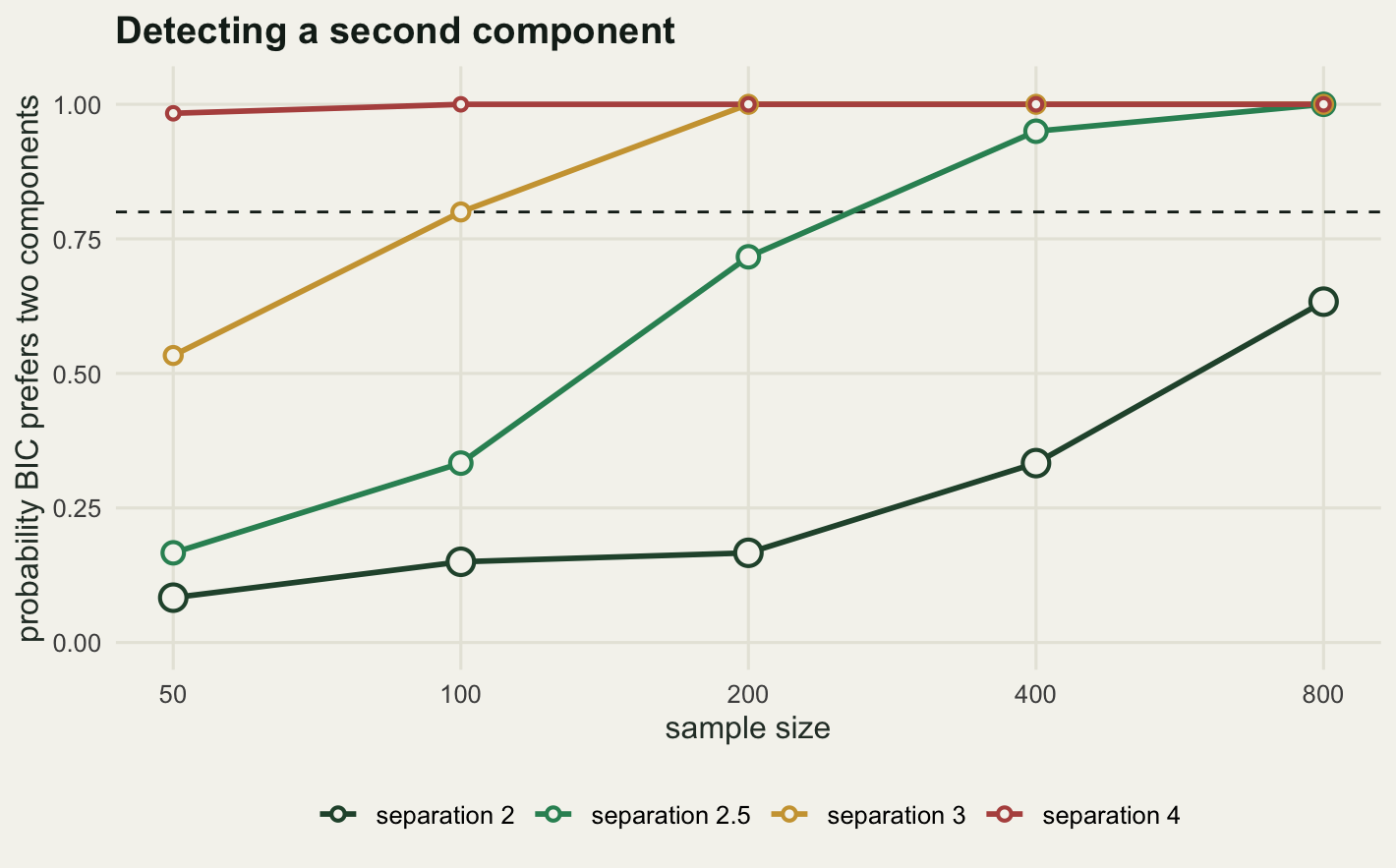
The optimism does not survive. At a separation of two standard deviations, which is exactly where bimodality appears, BIC prefers two components in 0.633 of replicates even with 800 observations, and the interpolated sample size for a probability of 0.8 is off the end of the grid. At a separation of 2.5 the interpolated requirement is about 256.2 observations. At 3.0 it is 100.0, and at 4.0 it is at or below 50.0, the smallest sample size in the grid.
Put those numbers next to the sample sizes ecologists actually have. A netting survey that yields 200 fish, a trapping season that yields 100 small mammals, a morphometric data set of 50 museum skins: at 200 observations the separation has to be around 2.5 before the second component is found reliably, which is more separation than bimodality needs, not less. The comfortable reading, that the likelihood sees structure the eye cannot, is backwards at these sample sizes. The eye sees a shoulder at a separation of two; the selection criterion needs to get to about 2.5 or 3.0 before it commits.
There is one honest qualification. This measures BIC specifically. AIC, from the previous section, picks up the two-component case at a separation of two far more often, at a rate of 0.617, and it pays for that with its over-selection rate on one-component data. The separation you can detect is not a property of the data; it is a property of the data plus the penalty you chose.
What unequal variances buy and cost
Every fit so far has forced the components to share a standard deviation. The unequal-variance family is more flexible and is the default in several packages, and the standard warning is that the extra freedom lets a spurious component attach itself to whatever is non-normal about the data. Test that by generating one-component data of three kinds, each standardised to unit variance: a clean normal, a skewed gamma with shape four, and a heavy-tailed t on five degrees of freedom. Then let BIC choose between one, two and three components within each family.
gen_e <- function(cond, n) {
  if (cond == "normal") rnorm(n)
  else if (cond == "skewed") (rgamma(n, 4, 1) - 4) / 2
  else rt(n, 5) / sqrt(5 / 3)
}

conds <- c("normal", "skewed", "heavy")
rep_g <- 80
n_f <- 200
set.seed(20260804)
grid_e <- NULL
for (cond in conds) {
  for (ev in c(TRUE, FALSE)) {
    khat <- integer(rep_g)
    for (r in seq_len(rep_g)) {
      x <- gen_e(cond, n_f)
      khat[r] <- which.min(c(
        crit_all(fit_one(x), n_f)["bic"],
        crit_all(em_mix(x, 2, equal_var = ev, max_iter = 50), n_f)["bic"],
        crit_all(em_mix(x, 3, equal_var = ev, max_iter = 50, starts = 2), n_f)["bic"]))
    }
    grid_e <- rbind(grid_e, data.frame(
      shape = cond, family = ifelse(ev, "equal", "unequal"),
      over_selects = mean(khat > 1), picks_three = mean(khat == 3)))
  }
}
print(c(replicates_per_cell = rep_g, n = n_f, true_components = 1))
replicates_per_cell n true_components
80 200 1 print(data.frame(shape = grid_e$shape, family = grid_e$family,
over_selects = round(grid_e$over_selects, 4),
picks_three = round(grid_e$picks_three, 4))) shape family over_selects picks_three
1 normal equal 0.0000 0.0000
2 normal unequal 0.0000 0.0000
3 skewed equal 0.9500 0.1125
4 skewed unequal 0.9125 0.0750
5 heavy equal 0.1750 0.1750
6 heavy unequal 0.4375 0.0125diff_e <- grid_e$over_selects[c(2, 4, 6)] - grid_e$over_selects[c(1, 3, 5)]
print(round(setNames(diff_e, conds), 4)) normal skewed heavy
0.0000 -0.0375 0.2625 On clean normal data neither family over-selects: both sit at 0.0000. That is BIC doing its job, and it also confirms that the variance floor in the fitter is holding, because an unbounded unequal-variance likelihood would have produced spurious spike components here and it did not.
The other two conditions split the standard warning in half. On heavy-tailed data the warning is exactly right: the equal-variance family over-selects 0.1750 of the time and the unequal-variance family 0.4375, a difference of 0.2625. The extra component in the unequal-variance fit is a wide, low-weight component that swallows the tails, and it is cheap enough at one extra variance parameter that BIC accepts it often.
On skewed data the warning is wrong, and it is wrong in a way that matters more than the case where it is right. Both families over-select almost always: the equal-variance family at 0.9500 and the unequal-variance family at 0.9125, a difference of -0.0375, which is on the wrong side of zero. Constraining the variances gives no protection at all against skewness. With a common standard deviation the only way to bend a symmetric fit into a skewed shape is to shift a second mean sideways, which is precisely the spurious component, and BIC buys it 0.9500 of the time on data with one population in it.
That is the finding to carry out of this section, because it inverts the usual advice. Restricting to equal variances is often recommended as the cautious choice for deciding how many components there are. It is cautious against heavy tails and useless against skewness, and skewness is the more common shape in body sizes, seed masses, clutch sizes and almost every other positive measurement in ecology. The equal-variance family also picks three components more often than the unequal-variance one on heavy-tailed data, at 0.1750 against 0.0125, which is the same mechanism seen from the other side: with variances tied, it takes more components to cover the same departure from normality.
What to take away
The likelihood ratio test for the number of components does not have a chi-squared null distribution, and the way it fails is not the way the textbook warning suggests. Its distribution has a point mass at zero, at 0.1633 of replicates in the one against two comparison and 0.3067 in the two against three, and no degrees of freedom setting fits both the body and the tail. Choosing two degrees of freedom happened to give an error rate near nominal here, at 0.0467, but the same choice gave 0.0333 one level up, and the more careful-sounding choice of one degree of freedom gave 0.1167. If a test is what you want, the parametric bootstrap version measured at 0.0667 against a nominal five per cent, and it cost 100 EM fits per test.
If a criterion is what you want, the choice is between two kinds of error rather than between right and wrong. AIC over-selected at 0.0667 and BIC under-selected at 0.1750 on the same grid, and AIC came out ahead on overall recovery, 0.8722 against 0.8222, because the grid contained a poorly separated cell where caution is expensive. ICL is answering a different question and should be read that way: it prefers components you could assign individuals to, which is why it selected one component at a separation of 3 even though the density genuinely had two and the classifier was already at its Bayes limit of 0.933.
The honest limit is larger than any of these results. The number of components is a property of a model, not of a population: no lake contains a number of normal components, and there is no sample size at which the question becomes safe, because every one of the criteria above is comparing candidate models rather than testing nature. The measurements here show that the answer moves with the penalty, the variance family and the separation, and it moves by enough to change the conclusion. The question that survives is the applied one. If a two-component fit gives you cohort means you can defend and a growth curve that holds up against known-age fish, the fit has earned its second component. If the only evidence for it is that a criterion preferred it by a few units, the second component is a modelling choice being reported as a discovery.
References
McLachlan GJ 1987 Journal of the Royal Statistical Society Series C 36(3):318-324 (10.2307/2347790)
Biernacki C, Celeux G, Govaert G 2000 IEEE Transactions on Pattern Analysis and Machine Intelligence 22(7):719-725 (10.1109/34.865189)
Fraley C, Raftery AE 2002 Journal of the American Statistical Association 97(458):611-631 (10.1198/016214502760047131)
Feng ZD, McCulloch CE 1996 Journal of the Royal Statistical Society Series B 58(3):609-617 (10.1111/j.2517-6161.1996.tb02104.x)
Titterington DM, Smith AFM, Makov UE 1985 Statistical Analysis of Finite Mixture Distributions (ISBN 978-0-471-90763-3)
Dempster AP, Laird NM, Rubin DB 1977 Journal of the Royal Statistical Society Series B 39(1):1-22 (10.1111/j.2517-6161.1977.tb01600.x)