library(ggplot2)

te_pal <- list(forest = "#275139", green = "#2f8f63", sage = "#93a87f",
               clay = "#b5534e", gold = "#cda23f", line = "#dad9ca",
               ink = "#16241d", paper = "#f5f4ee")

theme_te <- function() {
  theme_minimal(base_size = 12) +
    theme(panel.grid.minor = element_blank(),
          panel.grid.major = element_line(colour = "#e7e6dc"),
          plot.background = element_rect(fill = "#f5f4ee", colour = NA),
          panel.background = element_rect(fill = "#f5f4ee", colour = NA),
          plot.title = element_text(face = "bold", colour = te_pal$ink),
          axis.title = element_text(colour = "#2c3a31"),
          legend.position = "bottom")
}When a mixture is really skewness
R
mixture models
model checking
ecology tutorial
Fit a two-component normal mixture to skewed ecological size data and BIC prefers it: measure how often that happens, what tells the two apart, and the cost.
The electrofishing survey finished on a Thursday and the masses went into a spreadsheet the same evening: a basin’s worth of roach, weighed to the tenth of a gram. The histogram that came back the next morning had the shape everyone expected, bunched up on the left with a thin tail running out to the right.
Somebody in the meeting said what people always say about that shape. Two cohorts. The young of the year sit in the bunch, the older fish are strung out along the tail, and a mixture model will pull them apart and give a proportion for each. That is a reasonable thing to say, and there is a well-tested tool for it. Fit a two-component normal mixture by EM, compare it with one component by BIC, take the winner.
The fit converged without complaint. It reported two components with clearly different means, sensible standard deviations, and a decent weight on the larger one. BIC preferred it over the single normal by a margin that is as decisive as model selection ever gets.
There were no cohorts. The masses were drawn from a single log-normal distribution with no group structure of any kind. This post measures how easily that happens, what it costs a decision that depends on the fit, and which of the usual diagnostics actually tells the two situations apart. The short version, measured rather than asserted: the classification entropy people reach for first is the weakest of the candidates tested, and the log-normal with no components in it looks to BIC like a genuine mixture whose components sit almost four standard deviations apart.
Earlier posts supply the machinery and it is not repeated here. Fitting a mixture of normals in R builds the EM fitter, and How many components in a mixture? covers the selection criteria and their behaviour on the boundary. The fitter below is a compact version of the same algorithm, with a variance floor so that no component can collapse onto a single observation.
A sample with no groups in it
The fitter is the standard two-component EM loop: compute the responsibility of the first component for each observation, then update the weight, the two means and the two standard deviations as responsibility-weighted moments. The only addition is a floor on each standard deviation, set at a fixed fraction of the sample standard deviation, because without it the likelihood of a normal mixture is unbounded: a component can sit on one point with a vanishing variance and drive the density there to infinity. Starts from several different quantile pairs guard against the poorer local optima.
em_two <- function(x, start, iter = 400, tol = 1e-8, floor_frac = 0.1) {
  n <- length(x)
  sx <- sqrt(sum((x - mean(x))^2) / n)
  mu <- start
  sg <- rep(sx / 1.5, 2)
  wt <- 0.5
  fl <- floor_frac * sx
  ll_old <- -Inf; ll <- -Inf
  for (i in seq_len(iter)) {
    d1 <- wt * dnorm(x, mu[1], sg[1])
    d2 <- (1 - wt) * dnorm(x, mu[2], sg[2])
    tot <- pmax(d1 + d2, 1e-300)
    r <- d1 / tot
    ll <- sum(log(tot))
    n1 <- sum(r)
    n2 <- n - n1
    wt <- n1 / n
    mu[1] <- sum(r * x) / n1
    mu[2] <- sum((1 - r) * x) / n2
    sg[1] <- max(sqrt(sum(r * (x - mu[1])^2) / n1), fl)
    sg[2] <- max(sqrt(sum((1 - r) * (x - mu[2])^2) / n2), fl)
    if (abs(ll - ll_old) < tol * (abs(ll) + 1)) break
    ll_old <- ll
  }
  if (mu[1] > mu[2]) { mu <- rev(mu); sg <- rev(sg); wt <- 1 - wt }
  list(mu = mu, sg = sg, wt = wt, loglik = ll)
}

fit_two <- function(x, nstart = 3) {
  qq <- as.numeric(quantile(x, c(0.10, 0.90, 0.30, 0.70, 0.02, 0.60)))
  best <- NULL
  for (s in seq_len(nstart)) {
    f <- em_two(x, qq[c(2 * s - 1, 2 * s)])
    if (is.null(best) || f$loglik > best$loglik) best <- f
  }
  best
}

fit_one <- function(x) {
  m <- mean(x); s <- sqrt(sum((x - m)^2) / length(x))
  list(mu = m, sg = s, loglik = sum(dnorm(x, m, s, log = TRUE)))
}

fit_lnorm <- function(x) {
  m <- mean(log(x)); s <- sqrt(sum((log(x) - m)^2) / length(x))
  list(ml = m, sl = s, loglik = sum(dlnorm(x, m, s, log = TRUE)))
}

bic_of <- function(loglik, k, n) -2 * loglik + k * log(n)

dmix <- function(x, f) {
  f$wt * dnorm(x, f$mu[1], f$sg[1]) + (1 - f$wt) * dnorm(x, f$mu[2], f$sg[2])
}

pmix <- function(q, f) {
  f$wt * pnorm(q, f$mu[1], f$sg[1]) + (1 - f$wt) * pnorm(q, f$mu[2], f$sg[2])
}

rmix <- function(n, mu, sg, wt) {
  k <- 1 + (runif(n) > wt)
  rnorm(n, mu[k], sg[k])
}
The data are one log-normal draw. Setting the log-scale standard deviation to 0.55 and the median mass to 12 grams gives the kind of right skew that body mass, seed weight, patch area and territory size all show. There is one population, one mechanism, and no latent label anywhere in the generating code.
set.seed(20260729)
mlog <- log(12)
slog <- 0.55
n_obs <- 400
masses <- rlnorm(n_obs, mlog, slog)

fit2 <- fit_two(masses); fit1 <- fit_one(masses)
bic_two <- bic_of(fit2$loglik, 5, n_obs)
bic_one <- bic_of(fit1$loglik, 2, n_obs)
bic_gain <- bic_one - bic_two

print(round(c(mu_small = fit2$mu[1], mu_large = fit2$mu[2],
              sd_small = fit2$sg[1], sd_large = fit2$sg[2],
              weight_small = fit2$wt, weight_large = 1 - fit2$wt), 4))
mu_small mu_large sd_small sd_large weight_small weight_large
10.3181 22.9536 4.1336 9.1116 0.7977 0.2023 print(round(c(loglik_one = fit1$loglik, loglik_two = fit2$loglik,
bic_one = bic_one, bic_two = bic_two, bic_gain = bic_gain,
sample_mean = mean(masses), sample_sd = sd(masses),
n_obs = n_obs, median_mass = exp(mlog), log_sd = slog,
sd_floor_fraction = 0.1), 4)) loglik_one loglik_two bic_one bic_two
-1373.3486 -1301.7891 2758.6802 2633.5354
bic_gain sample_mean sample_sd n_obs
125.1447 12.8749 7.5059 400.0000
median_mass log_sd sd_floor_fraction
12.0000 0.5500 0.1000 The fit is clean. The smaller component sits at 10.3181 grams with a standard deviation of 4.1336, the larger at 22.9536 grams with a standard deviation of 9.1116, and the larger component carries a weight of 0.2023. Written up, that is a statement about the population: a sizeable minority of the fish in this basin belong to an older, heavier group whose mean mass is far above that of the young fish. Every part of that sentence is false, and nothing in the fit says so.
BIC is not close. The one-component fit scores 2758.6802 and the two-component fit scores 2633.5354, a gain of 125.1447 in favour of two components. Model selection differences of that size are usually reported as conclusive.
There is one thing in the output that ought to give pause, and it is easy to miss. The weighted components overlap so heavily that the fitted mixture density has only one peak.
grid_mode <- seq(0.1, 70, length.out = 3000)
dens_mode <- dmix(grid_mode, fit2)
m_last <- length(dens_mode)
n_peaks <- sum(dens_mode[2:(m_last - 1)] > dens_mode[1:(m_last - 2)] &
               dens_mode[2:(m_last - 1)] > dens_mode[3:m_last])
mass_neg <- pmix(0, fit2)

print(round(c(peaks_in_fitted_density = n_peaks,
              separation_in_pooled_sd = diff(fit2$mu) / sqrt(mean(fit2$sg^2)),
              mass_below_zero = mass_neg,
              fish_below_zero_per_400 = n_obs * mass_neg), 4))
peaks_in_fitted_density separation_in_pooled_sd mass_below_zero
1.0000 1.7860 0.0062
fish_below_zero_per_400
2.4788 The fitted density has 1 peak, not two. The means are separated by 1.786 pooled standard deviations, not enough to produce a visible dip, so a reader looking at the picture would never say “two humps”. The model says two components; the picture the model draws says one. That mismatch is the first useful signal, and it costs nothing to check.
The second signal is quieter. The fitted mixture places 0.0062 of its probability below zero, which is 2.4788 fish out of 400 with negative mass. A normal component reaching the right tail of a skewed distribution has to be broad, and a broad normal centred far up the axis leaks into the impossible region. No fish weighs less than nothing, so the model is already saying it has the wrong shape.
grid_plot <- seq(0, 55, length.out = 600)
lab_curve <- c("two-component total", "low-mass component",
               "high-mass component", "single normal")
curves <- data.frame(
  x = rep(grid_plot, 4),
  y = c(dmix(grid_plot, fit2),
        fit2$wt * dnorm(grid_plot, fit2$mu[1], fit2$sg[1]),
        (1 - fit2$wt) * dnorm(grid_plot, fit2$mu[2], fit2$sg[2]),
        dnorm(grid_plot, fit1$mu, fit1$sg)),
  curve = factor(rep(lab_curve, each = 600), levels = lab_curve))

ggplot() +
  geom_histogram(data = data.frame(m = masses), aes(x = m, y = after_stat(density)),
                 bins = 40, fill = te_pal$line, colour = te_pal$paper, linewidth = 0.3) +
  geom_line(data = curves, aes(x = x, y = y, colour = curve, linetype = curve),
            linewidth = 0.9) +
  scale_colour_manual(values = c("two-component total" = te_pal$forest,
                                 "low-mass component" = te_pal$clay,
                                 "high-mass component" = te_pal$gold,
                                 "single normal" = te_pal$sage), name = NULL) +
  scale_linetype_manual(values = c("two-component total" = "solid",
                                   "low-mass component" = "dashed",
                                   "high-mass component" = "dashed",
                                   "single normal" = "solid"), name = NULL) +
  labs(x = "mass (g)", y = "density",
       title = "A two-component fit to data with one component") +
  theme_te() +
  theme(plot.margin = margin(6, 12, 6, 6))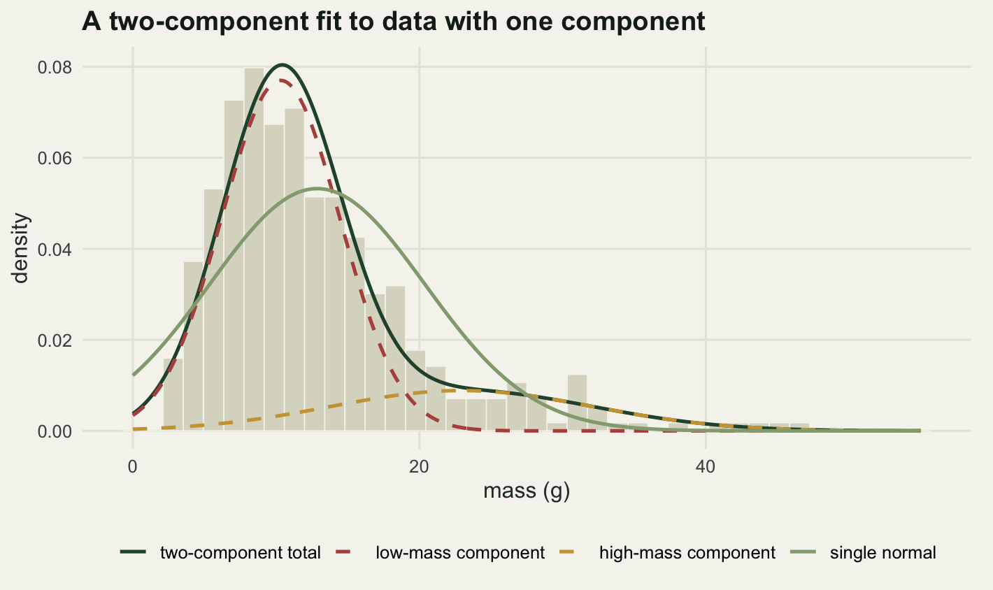
The picture is the reason this mistake survives peer review. The dark green curve is a good description of the histogram. It follows the rise, the peak and the tail better than the symmetric single normal does, which is exactly what the likelihood said. Nothing about it looks like a model that has invented a population.
How small a sample is safe
The obvious defence is sample size. Spurious structure is a large-sample problem, the argument goes, and BIC’s penalty grows with log(n), so a modest survey should be protected. That is testable: draw from the same log-normal at a range of sample sizes and count how often BIC prefers two components over one.
set.seed(41200729)
n_grid <- c(25, 40, 60, 100, 200, 400)
n_rep <- 120
prop_two <- numeric(length(n_grid)); med_gain <- numeric(length(n_grid))

for (j in seq_along(n_grid)) {
  gains <- numeric(n_rep)
  for (b in seq_len(n_rep)) {
    xx <- rlnorm(n_grid[j], mlog, slog)
    gains[b] <- bic_of(fit_one(xx)$loglik, 2, n_grid[j]) -
                bic_of(fit_two(xx)$loglik, 5, n_grid[j])
  }
  prop_two[j] <- mean(gains > 0)
  med_gain[j] <- median(gains)
}

sweep_tab <- data.frame(n = n_grid,
                        prop_two_components = round(prop_two, 3),
                        median_bic_gain = round(med_gain, 2),
                        replicates = n_rep)
print(sweep_tab)
n prop_two_components median_bic_gain replicates
1 25 0.567 0.62 120
2 40 0.708 2.64 120
3 60 0.850 9.17 120
4 100 0.992 19.05 120
5 200 1.000 52.86 120
6 400 1.000 119.74 120The defence does not hold. At 25 observations, a smaller sample than almost any published size-structure analysis, BIC already prefers two components in 0.567 of 120 replicates. By 100 it is 0.992, and from 200 onwards 1.000: every replicate, every time.
What changes with sample size is not whether the wrong model wins but how loudly. The median BIC gain runs from 0.62 at the smallest sample to 119.74 at 400. A small survey gets a marginal preference an author might report cautiously; a large survey gets one so large that caution would look like false modesty. Both are wrong in the same way, and the large one is wrong more persuasively.
The reason is arithmetic rather than anything subtle about mixtures. The extra parameters of the mixture cost a fixed multiple of log(n) in BIC, so their price grows like the logarithm of the sample size, while the log-likelihood advantage of the richer model grows linearly, because every new observation contributes its own share of the discrepancy between a skewed density and a symmetric one. Linear beats logarithmic past a small constant, and for a distribution this skewed that constant is smaller than any sample an ecologist would bother to collect.
The closest real mixture
If skewness alone can produce this, the next question is whether the two situations are distinguishable at all. Take the log-normal and find the two-component normal mixture that mimics it best, minimising the Kullback-Leibler divergence from the log-normal to the mixture. That is the same EM update as before, run on a fine grid with the log-normal density as the weights instead of on a sample. It converges to the population-level best imitation: no genuine mixture can hide behind this log-normal more successfully.
grid_proj <- seq(qlnorm(1e-7, mlog, slog), qlnorm(1 - 1e-7, mlog, slog), length.out = 4000)
d_step <- grid_proj[2] - grid_proj[1]
w_dens <- dlnorm(grid_proj, mlog, slog)
w_dens <- w_dens / sum(w_dens)

proj <- list(mu = c(9, 20), sg = c(3, 8), wt = 0.7)
for (i in 1:800) {
  d1 <- proj$wt * dnorm(grid_proj, proj$mu[1], proj$sg[1])
  d2 <- (1 - proj$wt) * dnorm(grid_proj, proj$mu[2], proj$sg[2])
  r <- d1 / pmax(d1 + d2, 1e-300)
  a1 <- sum(w_dens * r)
  a2 <- 1 - a1
  proj$wt <- a1
  proj$mu <- c(sum(w_dens * r * grid_proj) / a1,
               sum(w_dens * (1 - r) * grid_proj) / a2)
  proj$sg <- c(sqrt(sum(w_dens * r * (grid_proj - proj$mu[1])^2) / a1),
               sqrt(sum(w_dens * (1 - r) * (grid_proj - proj$mu[2])^2) / a2))
}

f_true <- dlnorm(grid_proj, mlog, slog)
g_proj <- dmix(grid_proj, proj)
tv_dist <- 0.5 * sum(abs(f_true - g_proj)) * d_step
i_gap <- which.max(abs(f_true - g_proj))
max_gap <- abs(f_true - g_proj)[i_gap]

print(round(c(mu_small = proj$mu[1], mu_large = proj$mu[2],
              sd_small = proj$sg[1], sd_large = proj$sg[2],
              weight_large = 1 - proj$wt), 4))
mu_small mu_large sd_small sd_large weight_large
10.7922 22.6507 4.2338 10.2691 0.2671 print(round(c(total_variation = tv_dist, max_gap = max_gap,
gap_at_mass = grid_proj[i_gap],
gap_as_fraction_of_density = max_gap / f_true[i_gap],
mixture_mass_below_zero = pmix(0, proj)), 5)) total_variation max_gap
0.09840 0.01571
gap_at_mass gap_as_fraction_of_density
6.32580 0.26979
mixture_mass_below_zero
0.00762 The best imitation is close to the fit obtained from the single sample of 400, which is reassuring about the fitter: the earlier result was not a fluke of one draw. The mimic has components at 10.7922 and 22.6507 grams, with a weight of 0.2671 on the larger.
The two densities are not identical. The total variation distance between them is 0.0984, the fraction of the probability mass that would have to be moved to turn one into the other. The largest vertical gap is 0.01571 in density units, at a mass of 6.3258 grams, where the mixture falls short of the log-normal by a fraction 0.26979 of the local density. That is a real difference on the left shoulder, and a plot of the two densities shows it plainly.
What it does not show is on a histogram of 400 points, where the sampling noise in each bin is larger than the gap. The difference is easy to see when you draw the densities and impossible to see when you draw the data.
keep <- grid_proj <= 50
lab_series <- c("log-normal", "closest two-component mixture",
                "mixture minus log-normal")
both <- data.frame(
  x = rep(grid_proj[keep], 3),
  y = c(f_true[keep], g_proj[keep], (g_proj - f_true)[keep]),
  series = factor(rep(lab_series, each = sum(keep)), levels = lab_series),
  panel = factor(rep(c("density", "density", "difference"), each = sum(keep)),
                 levels = c("density", "difference"),
                 labels = c("density", "difference in density (finer scale)")))

ggplot(both, aes(x = x, y = y, colour = series, linetype = series)) +
  geom_hline(yintercept = 0, colour = te_pal$line, linewidth = 0.4) +
  geom_line(linewidth = 0.9) +
  facet_wrap(~ panel, ncol = 1, scales = "free_y") +
  scale_colour_manual(values = c("log-normal" = te_pal$forest,
                                 "closest two-component mixture" = te_pal$clay,
                                 "mixture minus log-normal" = te_pal$gold),
                      name = NULL) +
  scale_linetype_manual(values = c("log-normal" = "solid",
                                   "closest two-component mixture" = "dashed",
                                   "mixture minus log-normal" = "solid"),
                        name = NULL) +
  guides(colour = guide_legend(nrow = 2), linetype = guide_legend(nrow = 2)) +
  labs(x = "mass (g)", y = NULL,
       title = "A skewed density and its best two-component imitation") +
  theme_te() +
  theme(plot.margin = margin(6, 12, 6, 6))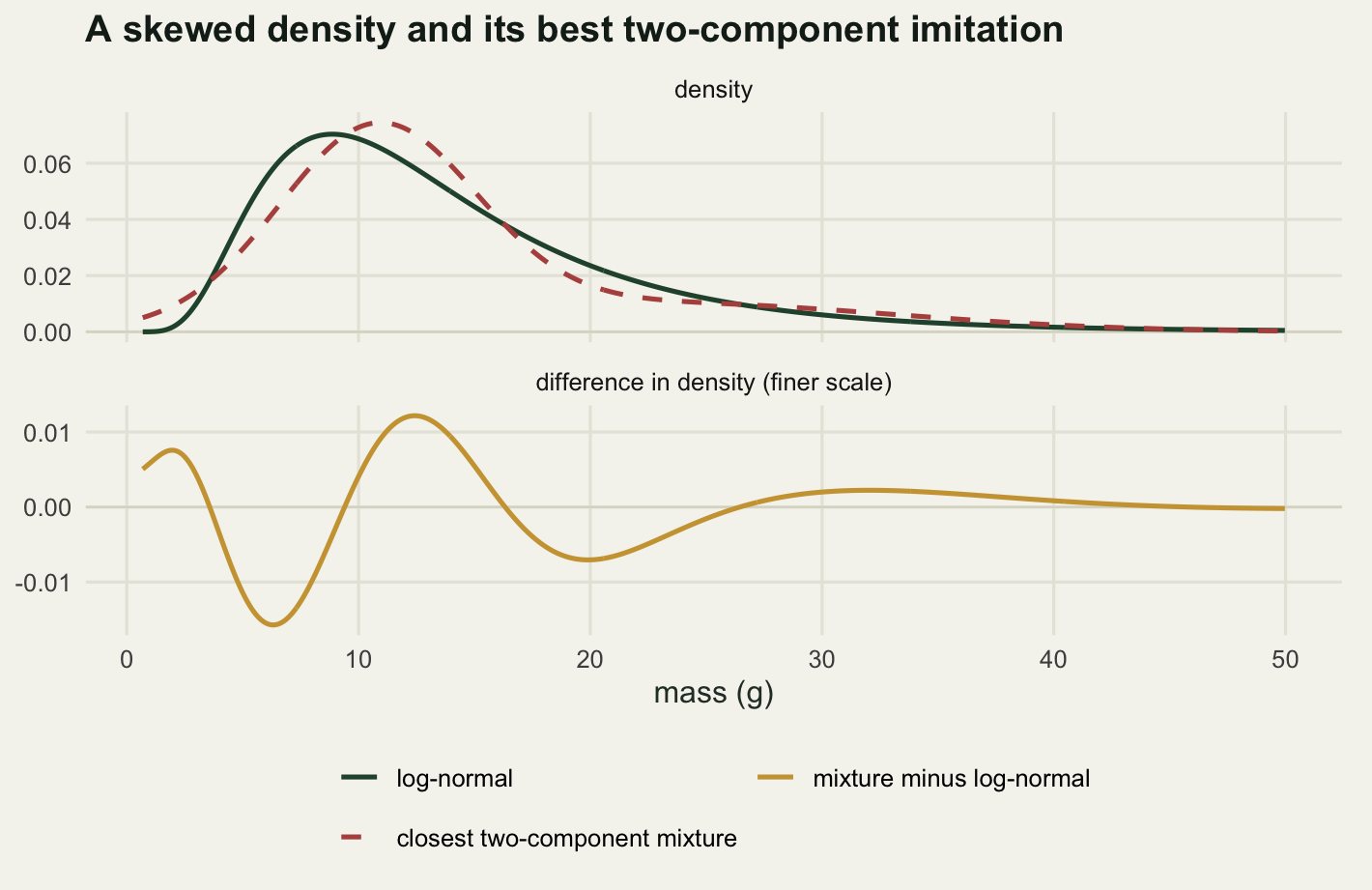
Now the sample size question, asked the other way round. Given a sample, can anything tell which of the two generating processes produced it? A sensible statistic is the difference in maximised log-likelihood between the two-component normal mixture and a single log-normal fitted to the same data: under log-normal data the mixture wins by little or loses, under mixture data it wins by more. Calibrate the cutoff on log-normal replicates so the false positive rate is 0.05, then count how often mixture-generated samples clear it. The mimic puts 0.00762 of its mass below zero, which cannot happen for a real size distribution, so the simulated mixture is truncated at zero by rejection first.
r_proj <- function(n) {
  out <- numeric(0)
  while (length(out) < n) {
    v <- rmix(2 * n, proj$mu, proj$sg, proj$wt)
    out <- c(out, v[v > 0])
  }
  out[seq_len(n)]
}

set.seed(88200729)
np_grid <- c(50, 100, 200, 400)
n_rep2 <- 120
power_lr <- numeric(length(np_grid))

for (j in seq_along(np_grid)) {
  n <- np_grid[j]
  t_null <- numeric(n_rep2); t_alt <- numeric(n_rep2)
  for (b in seq_len(n_rep2)) {
    x0 <- rlnorm(n, mlog, slog)
    t_null[b] <- fit_two(x0)$loglik - fit_lnorm(x0)$loglik
    x1 <- r_proj(n)
    t_alt[b] <- fit_two(x1)$loglik - fit_lnorm(x1)$loglik
  }
  power_lr[j] <- mean(t_alt > quantile(t_null, 0.95))
}

print(data.frame(n = np_grid, power = round(power_lr, 3), replicates = n_rep2))
n power replicates
1 50 0.425 120
2 100 0.850 120
3 200 0.975 120
4 400 1.000 120print(round(c(false_positive_rate = 0.05), 4))false_positive_rate
0.05 This is the first result that came out backwards. A total variation distance of 0.0984 looked, on a histogram, like something that would need thousands of observations to detect. It does not. Power reaches 0.85 at 100 observations and 0.975 at 200. At 50 observations the test is still weak, at 0.425, but by the sample sizes a typical fisheries or plant survey collects the two processes are separable.
The information was there the whole time; the histogram was the wrong instrument for reading it. Every observation contributes a small amount of evidence and the contributions add up linearly. What made the earlier fit go wrong was not a shortage of information but the absence of the log-normal from the set of models compared. Fitting two normals against one normal answers the question “is one normal enough”, and the answer to that is no. It was never the question anybody meant to ask.
Three ways to tell the two apart
The diagnostics that get recommended for exactly this problem can be put on the same footing and ranked. All are turned into a decision with a false positive rate of 0.05, calibrated on samples drawn from the log-normal, and then applied to samples from the truncated best-imitation mixture. The sample size is 120 throughout, which is nearer to a real survey than the 400 used above and makes the comparison harder.
The first candidate is the entropy of the classification. If two components are real, the posterior responsibility of each observation should be near zero or near one, and the average binary entropy of those responsibilities should be small. The normalised version below is one minus the mean entropy in bits, so it runs from zero for a fit that cannot classify anything to one for a fit that classifies everything with certainty. The second is the model comparison the previous section already used: BIC for a single log-normal against BIC for a two-component normal mixture.
The third is a second measurement. Suppose that alongside mass there is a variable that ought to differ between the putative groups if the groups are real: an otolith reading, a stable isotope ratio, a capture date. Assign each individual its posterior responsibility and correlate that with the second variable. If the grouping is an artefact of skewness the correlation is noise; if the groups are real and the second variable tracks them, it is not. Two effect sizes are tested, a difference of 1.5 standard deviations between the true components and a weaker difference of 0.75.
norm_entropy <- function(x, f) {
  d1 <- f$wt * dnorm(x, f$mu[1], f$sg[1])
  d2 <- (1 - f$wt) * dnorm(x, f$mu[2], f$sg[2])
  r <- pmin(pmax(d1 / pmax(d1 + d2, 1e-300), 1e-12), 1 - 1e-12)
  1 + sum(r * log(r) + (1 - r) * log(1 - r)) / (length(x) * log(2))
}

post_r <- function(x, f) {
  d1 <- f$wt * dnorm(x, f$mu[1], f$sg[1])
  d1 / pmax(d1 + (1 - f$wt) * dnorm(x, f$mu[2], f$sg[2]), 1e-300)
}

mu_sep <- c(10, 26); sg_sep <- c(2.5, 4); wt_sep <- 0.7

set.seed(51200729)
n_small <- 120
n_rep3 <- 200
ent_skew <- ent_match <- ent_sep <- numeric(n_rep3)
fam_skew <- fam_match <- numeric(n_rep3)
cov_skew <- cov_strong <- cov_weak <- numeric(n_rep3)

for (b in seq_len(n_rep3)) {
  x <- rlnorm(n_small, mlog, slog)
  fx <- fit_two(x)
  ent_skew[b] <- norm_entropy(x, fx)
  fam_skew[b] <- bic_of(fit_lnorm(x)$loglik, 2, n_small) -
                 bic_of(fx$loglik, 5, n_small)
  cov_skew[b] <- abs(cor(post_r(x, fx), rnorm(n_small)))

  y <- numeric(0); lab <- numeric(0)
  while (length(y) < n_small) {
    k <- 1 + (runif(2 * n_small) > proj$wt)
    v <- rnorm(2 * n_small, proj$mu[k], proj$sg[k])
    y <- c(y, v[v > 0]); lab <- c(lab, k[v > 0])
  }
  y <- y[seq_len(n_small)]; lab <- lab[seq_len(n_small)]
  fy <- fit_two(y)
  ry <- post_r(y, fy)
  ent_match[b] <- norm_entropy(y, fy)
  fam_match[b] <- bic_of(fit_lnorm(y)$loglik, 2, n_small) -
                  bic_of(fy$loglik, 5, n_small)
  cov_strong[b] <- abs(cor(ry, rnorm(n_small, 1.5 * (lab - 1), 1)))
  cov_weak[b] <- abs(cor(ry, rnorm(n_small, 0.75 * (lab - 1), 1)))

  s <- rmix(n_small, mu_sep, sg_sep, wt_sep)
  ent_sep[b] <- norm_entropy(s, fit_two(s))
}

print(round(c(entropy_skewed = mean(ent_skew), entropy_matched = mean(ent_match),
              entropy_separated = mean(ent_sep), n_small = n_small,
              replicates = n_rep3, sep_mu_small = mu_sep[1], sep_mu_large = mu_sep[2],
              sep_sd_small = sg_sep[1], sep_sd_large = sg_sep[2],
              effect_strong = 1.5, effect_weak = 0.75), 4))
entropy_skewed entropy_matched entropy_separated n_small
0.6262 0.7646 0.9764 120.0000
replicates sep_mu_small sep_mu_large sep_sd_small
200.0000 10.0000 26.0000 2.5000
sep_sd_large effect_strong effect_weak
4.0000 1.5000 0.7500 power_tab <- data.frame(
discriminator = c("classification entropy", "log-normal versus mixture by BIC",
"second variable, effect 1.5", "second variable, effect 0.75",
"classification entropy, separated mixture"),
power = round(c(mean(ent_match > quantile(ent_skew, 0.95)),
mean(fam_match > quantile(fam_skew, 0.95)),
mean(cov_strong > quantile(cov_skew, 0.95)),
mean(cov_weak > quantile(cov_skew, 0.95)),
mean(ent_sep > quantile(ent_skew, 0.95))), 3))
print(power_tab) discriminator power
1 classification entropy 0.285
2 log-normal versus mixture by BIC 0.880
3 second variable, effect 1.5 0.995
4 second variable, effect 0.75 0.710
5 classification entropy, separated mixture 0.995print(round(c(lognormal_wins_on_skewed_data = mean(fam_skew < 0),
median_bic_gap_on_skewed_data = median(fam_skew)), 4))lognormal_wins_on_skewed_data median_bic_gap_on_skewed_data
1.0000 -21.8346 The ranking is clear and it is not the one the folklore predicts. The second variable at an effect of 1.5 standard deviations is best, at 0.995, and the log-normal against the mixture by BIC is second, at 0.88. The second variable at the weaker effect of 0.75 comes third, at 0.71. Classification entropy is last by a wide margin, at 0.285, well above the 0.05 it would achieve by guessing but low enough that most real mixtures go undetected.
Entropy fails here for a reason worth understanding, because it is not a bad statistic in general. The mean normalised score is 0.6262 on skewed data and 0.7646 on the imitating mixture, a gap that leaves the two score distributions heavily overlapped at 120 observations. Run the same statistic against a mixture whose components really are far apart, at means of 10 and 26 with standard deviations of 2.5 and 4, and the score rises to 0.9764 and the power to 0.995.
pow_dat <- power_tab
pow_dat$zero <- 0
pow_dat$alternative <- c(rep("best-imitation mixture", 4), "well separated mixture")
pow_dat$discriminator <- factor(pow_dat$discriminator,
                                levels = pow_dat$discriminator[order(pow_dat$power)])

ggplot(pow_dat, aes(x = power, y = discriminator, colour = alternative)) +
  geom_segment(aes(x = zero, xend = power, yend = discriminator), linewidth = 1.1) +
  geom_point(size = 3.2) +
  geom_text(aes(label = sprintf("%.3f", power)), hjust = -0.3, size = 3.3,
            show.legend = FALSE) +
  scale_colour_manual(values = c("best-imitation mixture" = te_pal$forest,
                                 "well separated mixture" = te_pal$gold), name = NULL) +
  scale_x_continuous(limits = c(0, 1.18), breaks = seq(0, 1, 0.25)) +
  labs(x = "power at a false positive rate of 0.05", y = NULL,
       title = "What separates a real mixture from skewness") +
  theme_te() +
  theme(plot.margin = margin(6, 16, 6, 6))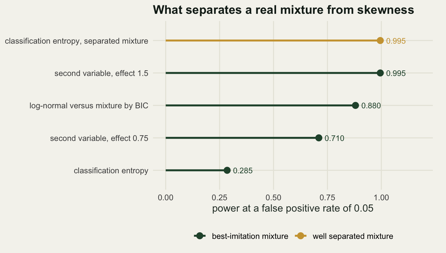
So entropy measures separation, not existence. A real but overlapping mixture and a fitted-to-skewness mixture both produce uncertain classifications, and nothing in the entropy tells those apart. Reporting a low entropy as evidence that a mixture is genuine is reading the wrong quantity.
The BIC comparison against a log-normal does much better. On all 200 skewed replicates the log-normal beat the two-component normal mixture, a proportion of 1.0000, with a median gap of -21.8346 BIC units. Add one sensible skewed family to the comparison set and the failure from the opening section disappears. That comes with a condition attached, and the condition is the honest limit of the whole approach: it only works if the family you added is the right one. The next chunk generates data from two other skewed distributions with no components in them, a gamma and a Weibull, both matched to the mean and standard deviation of the log-normal, and fits the same log-normal against the same mixture.
set.seed(66200729)
mean_target <- 13.9594; sd_target <- 8.2963
g_shape <- (mean_target / sd_target)^2
g_rate <- mean_target / sd_target^2
w_shape <- 1.6
w_scale <- mean_target / gamma(1 + 1 / w_shape)
n_rep4 <- 120; n_wrong <- 400
gain_gamma <- numeric(n_rep4); gain_weib <- numeric(n_rep4)

for (b in seq_len(n_rep4)) {
  xg <- rgamma(n_wrong, g_shape, g_rate)
  gain_gamma[b] <- bic_of(fit_lnorm(xg)$loglik, 2, n_wrong) -
                   bic_of(fit_two(xg)$loglik, 5, n_wrong)
  xw <- rweibull(n_wrong, w_shape, w_scale)
  gain_weib[b] <- bic_of(fit_lnorm(xw)$loglik, 2, n_wrong) -
                  bic_of(fit_two(xw)$loglik, 5, n_wrong)
}

print(round(c(gamma_shape = g_shape, gamma_skewness = 2 / sqrt(g_shape),
              weibull_shape = w_shape, n_wrong = n_wrong, replicates = n_rep4), 4))
gamma_shape gamma_skewness weibull_shape n_wrong replicates
2.8312 1.1886 1.6000 400.0000 120.0000 print(round(c(mixture_wins_on_gamma = mean(gain_gamma > 0),
median_gain_on_gamma = median(gain_gamma),
mixture_wins_on_weibull = mean(gain_weib > 0),
median_gain_on_weibull = median(gain_weib)), 4)) mixture_wins_on_gamma median_gain_on_gamma mixture_wins_on_weibull
0.1833 -15.9387 0.8667
median_gain_on_weibull
22.7984 Gamma data are handled reasonably: the mixture beats the fitted log-normal in only 0.1833 of 120 replicates, with a median gap of -15.9387 BIC units in the log-normal’s favour. The gamma is less skewed than the log-normal, its skewness being 1.1886, and a log-normal fitted to it is close enough to hold the line.
The Weibull is a different story. With a shape of 1.6 the density is right-skewed but its tail is much lighter than a log-normal’s, and a log-normal fitted to it is a poor description in exactly the region where the mixture’s second component is free to help. The mixture wins on 0.8667 of replicates, with a median gap of 22.7984 BIC units the wrong way. Add the wrong skewed family to the comparison and you are back where you started, with a confident two-component answer for data that has one component.
Where the fitter’s threshold actually is
The rule people carry in their heads is that two normal components with equal weights produce a visibly bimodal density only when their means are more than about two standard deviations apart. It is worth checking rather than quoting, and then worth comparing with the threshold the fitter uses. The first part is deterministic: for a given weight and separation, count the peaks of the mixture density on a fine grid and bisect on the separation until the count changes.
n_peaks_of <- function(delta, wt) {
  gg <- seq(-5, delta + 5, length.out = 4000)
  y <- wt * dnorm(gg) + (1 - wt) * dnorm(gg, delta)
  m <- length(y)
  sum(y[2:(m - 1)] > y[1:(m - 2)] & y[2:(m - 1)] > y[3:m])
}

bimodal_at <- function(wt, lo = 1.5, hi = 9) {
  for (i in 1:45) {
    mid <- (lo + hi) / 2
    if (n_peaks_of(mid, wt) >= 2) hi <- mid else lo <- mid
  }
  (lo + hi) / 2
}

wt_grid <- c(0.50, 0.40, 0.30, 0.20, 0.10, 0.05)
thresholds <- vapply(wt_grid, bimodal_at, numeric(1))
print(data.frame(minor_weight = wt_grid,
                 bimodal_threshold_sd = round(thresholds, 4)))
minor_weight bimodal_threshold_sd
1 0.50 2.0000
2 0.40 2.4427
3 0.30 2.7146
4 0.20 2.9807
5 0.10 3.3145
6 0.05 3.5806At equal weights the threshold is 2.0000 standard deviations, which confirms the rule of thumb exactly rather than approximately: one of the few round numbers in this area that is genuinely exact. The threshold rises quickly once the weights are unequal. At a minor weight of 0.3 it takes 2.7146 standard deviations to produce a second peak, and at a minor weight of 0.05 it takes 3.5806. A rare component has to be far away before it can raise a bump of its own, because it is competing against the shoulder of a much taller neighbour. Any real ecological mixture with an uncommon second group is therefore unimodal unless the groups barely overlap.
Now the fitter’s threshold. Simulate equal-weight, equal-variance two-component mixtures at a range of separations, with 400 observations each, and count how often BIC prefers two components over one. This uses a faster version of the EM loop, capped at a lower iteration count with a looser tolerance, because heavily overlapping components make the full EM crawl and the decision never changes.
fit_two_fast <- function(x) {
  qq <- as.numeric(quantile(x, c(0.15, 0.85, 0.35, 0.65)))
  a <- em_two(x, qq[1:2], iter = 150, tol = 1e-7)
  b <- em_two(x, qq[3:4], iter = 150, tol = 1e-7)
  if (b$loglik > a$loglik) b else a
}

set.seed(77200729)
d_grid <- c(1.0, 1.5, 2.0, 2.25, 2.5, 3.0, 3.5, 4.0, 4.5)
n_delta <- 400; n_rep5 <- 100
detect <- numeric(length(d_grid)); gain_delta <- numeric(length(d_grid))

for (j in seq_along(d_grid)) {
  gv <- numeric(n_rep5)
  for (b in seq_len(n_rep5)) {
    x <- rmix(n_delta, c(0, d_grid[j]), c(1, 1), 0.5)
    gv[b] <- bic_of(fit_one(x)$loglik, 2, n_delta) -
             bic_of(fit_two_fast(x)$loglik, 5, n_delta)
  }
  detect[j] <- mean(gv > 0)
  gain_delta[j] <- median(gv)
}

print(data.frame(delta = d_grid, prop_two = round(detect, 3),
                 median_bic_gain = round(gain_delta, 2), replicates = n_rep5))
delta prop_two median_bic_gain replicates
1 1.00 0.00 -16.53 100
2 1.50 0.01 -14.64 100
3 2.00 0.10 -7.63 100
4 2.25 0.41 -1.25 100
5 2.50 0.90 7.47 100
6 3.00 1.00 34.42 100
7 3.50 1.00 73.71 100
8 4.00 1.00 121.40 100
9 4.50 1.00 176.27 100cross_at <- function(yv, xv, target) {
i <- which(yv >= target)[1]
xv[i - 1] + (target - yv[i - 1]) * (xv[i] - xv[i - 1]) / (yv[i] - yv[i - 1])
}
delta_half <- cross_at(detect, d_grid, 0.5)
delta_equiv <- cross_at(gain_delta, d_grid, med_gain[length(n_grid)])
print(round(c(delta_for_half_detection = delta_half,
delta_matching_lognormal_gain = delta_equiv,
bimodality_threshold = thresholds[1],
lognormal_median_gain = med_gain[length(n_grid)],
n_per_replicate = n_delta), 4)) delta_for_half_detection delta_matching_lognormal_gain
2.2959 3.9826
bimodality_threshold lognormal_median_gain
2.0000 119.7396
n_per_replicate
400.0000 This is the second result that came out backwards. The expectation was that the fitter would be far more sensitive than the eye, reporting two components long before any dip appeared in the density. For a genuine symmetric mixture it is not. BIC picks two components in half the replicates at a separation of 2.2959 standard deviations, which is slightly above the bimodality threshold of 2.0000, not below it. At a separation of exactly two standard deviations, where the density has just acquired a second peak, BIC finds it in only 0.10 of replicates.
Put the two facts together and the picture changes shape. A real, equally weighted mixture whose components are two standard deviations apart is detected 0.10 of the time at 400 observations, while a log-normal with no components at all is detected every time, with a median BIC gain of 119.74. Reading that gain back onto the separation axis, the log-normal is as convincing to BIC as a genuine mixture separated by 3.9826 standard deviations.
That is what the criterion is actually doing. It is not measuring whether there are two groups; it is measuring departure from a single normal, and skewness is a much larger departure than a modest symmetric split. A distribution with zero components and a long right tail looks more non-normal than a real pair of overlapping groups, so it wins by more.
det_dat <- data.frame(delta = d_grid, prop = detect)

ggplot(det_dat, aes(x = delta, y = prop)) +
  annotate("segment", x = thresholds[1], xend = thresholds[1], y = 0, yend = 1.02,
           colour = te_pal$clay, linetype = "dashed", linewidth = 0.8) +
  annotate("segment", x = delta_equiv, xend = delta_equiv, y = 0, yend = 1.02,
           colour = te_pal$gold, linetype = "dashed", linewidth = 0.8) +
  annotate("text", x = thresholds[1] - 0.08, y = 0.72, hjust = 1, size = 3.4,
           colour = te_pal$clay, label = "density becomes\nbimodal") +
  annotate("text", x = delta_equiv - 0.08, y = 0.35, hjust = 1, size = 3.4,
           colour = te_pal$gold, label = "log-normal is this\nconvincing to BIC") +
  geom_line(colour = te_pal$forest, linewidth = 0.9) +
  geom_point(colour = te_pal$forest, size = 2.4) +
  scale_y_continuous(limits = c(-0.02, 1.06)) +
  scale_x_continuous(limits = c(0.8, 4.7)) +
  labs(x = "separation between component means (standard deviations)",
       y = "proportion choosing two components",
       title = "What BIC needs before it reports two components") +
  theme_te() +
  theme(plot.margin = margin(6, 14, 6, 6))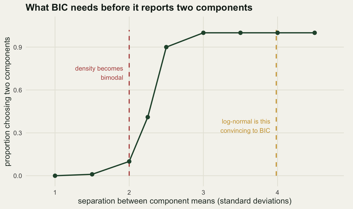
The gold line is the part to take away. It sits well to the right of the separation at which the detection curve has already reached one, in territory where a real mixture would be obviously bimodal and nobody would need a model selection criterion at all. The evidence the opening fit produced was not evidence for two overlapping groups; it was evidence for two groups so distinct they would have been visible from across the room, and there were none.
What the mistake costs
None of this matters unless a decision depends on it. Take one that does. A minimum landing size of 25 grams is in force, and the management question is what fraction of the population sits above it, which drives the expected catch and the quota. Estimate that fraction from the true log-normal, which sets the target but is unavailable in practice, from a fitted log-normal, and from the two-component mixture that BIC chose.
set.seed(99200729)
size_limit <- 25; far_limit <- 40
n_rep6 <- 150; n_dn <- 400
truth <- 1 - plnorm(c(size_limit, far_limit), mlog, slog)
est <- matrix(NA_real_, n_rep6, 4)
q_upper <- matrix(NA_real_, n_rep6, 2); w_large <- numeric(n_rep6)
grid_q <- seq(0, 200, length.out = 20000)

for (b in seq_len(n_rep6)) {
  x <- rlnorm(n_dn, mlog, slog)
  f2 <- fit_two(x); fl <- fit_lnorm(x)
  est[b, 1:2] <- 1 - pmix(c(size_limit, far_limit), f2)
  est[b, 3:4] <- 1 - plnorm(c(size_limit, far_limit), fl$ml, fl$sl)
  q_upper[b, 1] <- grid_q[which.min(abs(pmix(grid_q, f2) - 0.95))]
  q_upper[b, 2] <- qlnorm(0.95, fl$ml, fl$sl)
  w_large[b] <- 1 - f2$wt
}

print(round(c(true_fraction_above_25 = truth[1],
              mixture_estimate = mean(est[, 1]),
              lognormal_estimate = mean(est[, 3]),
              mixture_error_percent = 100 * (mean(est[, 1]) / truth[1] - 1),
              lognormal_error_percent = 100 * (mean(est[, 3]) / truth[1] - 1)), 4))
true_fraction_above_25 mixture_estimate lognormal_estimate
0.0910 0.1069 0.0909
mixture_error_percent lognormal_error_percent
17.4687 -0.1042 print(round(c(true_fraction_above_40 = truth[2],
mixture_estimate = mean(est[, 2]),
lognormal_estimate = mean(est[, 4]),
mixture_error_percent = 100 * (mean(est[, 2]) / truth[2] - 1),
lognormal_error_percent = 100 * (mean(est[, 4]) / truth[2] - 1)), 4)) true_fraction_above_40 mixture_estimate lognormal_estimate
0.0143 0.0124 0.0145
mixture_error_percent lognormal_error_percent
-13.3409 1.5604 print(round(c(upper_quantile = 0.95,
true_quantile_mass = qlnorm(0.95, mlog, slog),
mixture_estimate = mean(q_upper[, 1]),
lognormal_estimate = mean(q_upper[, 2]),
reported_weight_of_large_group = mean(w_large),
sd_of_reported_weight = sd(w_large),
replicates = n_rep6, n_dn = n_dn,
size_limit = size_limit, far_limit = far_limit), 4)) upper_quantile true_quantile_mass
0.9500 29.6534
mixture_estimate lognormal_estimate
31.3992 29.6530
reported_weight_of_large_group sd_of_reported_weight
0.2713 0.0814
replicates n_dn
150.0000 400.0000
size_limit far_limit
25.0000 40.0000 The true fraction above the landing size is 0.091. The fitted log-normal recovers 0.0909, an error of -0.1042 per cent, which is what an unbiased estimator with 400 observations should look like. The two-component mixture returns 0.1069, an error of 17.4687 per cent. A survey that reports the harvestable fraction that far high is not making a subtle mistake; it is the difference between a quota that holds and one that does not.
The sign flips further out. Above 40 grams the truth is 0.0143 and the mixture gives 0.0124, an error of -13.3409 per cent, this time an underestimate. A normal component, however broad, has a tail that dies like the exponential of a square, and no amount of fitting will make it match a log-normal tail. The mixture buys accuracy in the shoulder by borrowing from the extreme, a poor trade if the extreme is the trophy fish, the seed that disperses furthest or the patch large enough to hold a breeding pair. The overestimate returns a little closer in: the mass below which a fraction 0.95 of the population lies is 29.6534 grams, the fitted log-normal says 29.653 and the mixture pushes it out to 31.3992.
The worst output is not a number at all. Across 150 replicates the mixture reports a large-fish group carrying a mixture weight of 0.2713, with a standard deviation across replicates of 0.0814, about thirty per cent of the weight itself. That group would go into the results table, into a figure with two shaded densities, and quite possibly into a management plan as a stock component with its own catch-at-age line. It does not exist, and the fact that it turns up in every replicate is exactly what makes it look real.
What to take away
Fit two normal components to a skewed distribution and they will separate, converge and win on BIC. That is not a bug in the fitter or a failure of the criterion. Both are doing what they were asked: finding the best two-normal description of the data and asking whether it beats the best one-normal description. It does, because a skewed density is not one normal. The error is in the comparison set, not in the algorithm.
The measurements point at a few practical habits. Put at least one skewed single-component family into the comparison before you accept a mixture; on skewed data the log-normal beat the two-component mixture on 1.0000 of 200 replicates at only 120 observations. Check whether the fitted mixture density is actually bimodal, because the one in the opening section is not, and a fitted mixture that draws a single hump is describing shape rather than groups. Do not read low classification entropy as evidence of real components; its power against the hardest alternative here was 0.285, and it measures separation rather than existence.
The honest limit is the Weibull result. No statistic computed on a single variable can establish that a mixture is real, because the defence that works, comparing against a skewed family, requires you to have guessed the right skewed family: with a log-normal in the comparison set the two-component mixture still won on 0.8667 of Weibull-generated samples that had no components in them. The comparison set is always finite and the space of skewed shapes is not. What resolves the question is a second measurement, an otolith, an isotope ratio, a genotype, which had the highest power of anything tested here at 0.995, or knowing from the biology that two groups exist before the data are collected. The single-variable histogram cannot settle it, and the model selection output should not be read as though it had.
The replicate counts here are modest and printed with the results: 120 for the sample size sweep, 120 for the power curve, 200 for the discriminators, 120 for the wrong-family check, 100 for the separation sweep and 150 for the downstream costs. They are enough to rank the effects, and no single proportion should be read to its last digit.
References
McLachlan GJ, Lee SX, Rathnayake SI 2019 Annual Review of Statistics and Its Application 6:355-378 (10.1146/annurev-statistics-031017-100325)
Titterington DM, Smith AFM, Makov UE 1985 Statistical Analysis of Finite Mixture Distributions (ISBN 978-0-471-90763-3)
Schwarz G 1978 Annals of Statistics 6(2):461-464 (10.1214/aos/1176344136)
Fraley C, Raftery AE 2002 Journal of the American Statistical Association 97(458):611-631 (10.1198/016214502760047131)
Limpert E, Stahel WA, Abbt M 2001 BioScience 51(5):341-352 (10.1641/0006-3568(2001)051[0341:LNDATS]2.0.CO;2)
Celeux G, Soromenho G 1996 Journal of Classification 13(2):195-212 (10.1007/BF01246098)
Cassie RM 1954 Australian Journal of Marine and Freshwater Research 5(3):513-522 (10.1071/MF9540513)