library(ggplot2)
library(patchwork)

te_paper  <- "#f5f4ee"
te_ink    <- "#16241d"
te_body   <- "#2c3a31"
te_forest <- "#275139"
te_rust   <- "#b5534e"
te_gold   <- "#c9b458"
te_line   <- "#dad9ca"

theme_datasheet <- function() {
  theme_minimal(base_size = 12) +
    theme(plot.background  = element_rect(fill = te_paper, colour = NA),
          panel.background = element_rect(fill = te_paper, colour = NA),
          panel.grid.major = element_line(colour = te_line, linewidth = 0.3),
          panel.grid.minor = element_blank(),
          text             = element_text(colour = te_body),
          plot.title       = element_text(colour = te_ink, face = "bold"),
          plot.subtitle    = element_text(colour = te_body),
          axis.text        = element_text(colour = te_body),
          strip.text       = element_text(colour = te_ink))
}Bout-ending criteria and the histogram bin width
R
animal behaviour
biologging
mixture models
maximum likelihood
simulation
ecology tutorial
A bout-ending criterion fitted to binned log frequencies moves with bin width and sample size. Simulating behaviour bouts in R; the likelihood fit holds steady.
A time-depth recorder on a diving seabird returns a few thousand dives, and the first question after cleaning is how many foraging bouts they make. The bird dives, rests on the surface for a few seconds, dives again, and after a run of such dives flies off or sits on the water for a quarter of an hour. The same structure appears in the gaps between pecks at a feeder, between visits of a cow to a transponder trough and between calls of a singing bird. The analyst needs one number from the record: the gap length beyond which a new bout starts. Every later statistic, from bout duration to dives per bout, is counted with it.
The standard recipe treats the gaps as a mixture of two exponential distributions, a fast within-bout process and a slow between-bout process, and derives the bout-ending criterion from the fitted parameters. Sibly, Nott and Fletcher (1990) fitted the two processes by nonlinear regression to the logarithm of a histogram of gap lengths. Langton, Collett and Sibly (1995) fitted the same mixture by maximum likelihood to the gaps themselves, and Luque and Guinet (2007) compared a histogram-based method with maximum likelihood on fur seal dive records and simulated data, and found that the histogram bin width shifted the criterion. None of that is new here. This post is a demonstration of those results with its own grid of bin widths, rate ratios and sample sizes, and it adds one piece of mechanism: why the histogram fit moves, and what it moves towards.
The neighbours on this site stop one step earlier. Fitting a mixture of normals in R separates the components of a length sample by EM and uses the posterior memberships; it never needs a threshold between them. Here the number that matters is that threshold, and whether it is read from a histogram or from the gaps decides how many bouts the animal is said to have had. Checking an acoustic monitoring analysis simulates calls in bouts to show that bouts break the recorder-hour as a unit, but its bouts are known and never delimited. Accelerometer windows and short behaviours measures how window length caps the recall of short behaviours, a ratio of bout length to window with no criterion involved, and Behaviour sequences as Markov chains works with states and their durations rather than the gaps between events.
Which criterion, and its true value
A bout-ending criterion is a rule, and several rules exist. The one used throughout this post picks the gap length that minimises the total number of misassigned gaps: within-bout gaps longer than the criterion, which wrongly start a new bout, plus between-bout gaps shorter than it, which wrongly merge two bouts. Slater and Lester (1982) argued for minimising misassignments in this way. Write p for the share of within-bout gaps, f for the fast rate and s for the slow rate. The expected share of misassigned gaps at a criterion t is p exp(-f t) + (1 - p)(1 - exp(-s t)), and setting its derivative to zero gives
t = log(p f / ((1 - p) s)) / (f - s),
which is the point where the two weighted exponential densities cross. The same formula is applied to the true parameters, to give the truth, and to every set of fitted parameters, to give an estimate, so every ratio below compares like with like.
The design constants are fixed before anything is fitted: a within-bout mean gap of 10 s, a within-bout share of 0.95, 1000 gaps per animal, and a slow process whose mean gap is 20, 100 or 500 times longer than the fast one.
f_in   <- 0.1
p_in   <- 0.95
n_gap  <- 1000
ratios <- c(20, 100, 500)
bins   <- c(2, 10, 30)

bec <- function(p, f, s) log(p * f / ((1 - p) * s)) / (f - s)
mis_expected <- function(tc, p, f, s) p * exp(-f * tc) + (1 - p) * (1 - exp(-s * tc))

truth_tab <- data.frame(ratio = ratios, slow_mean = ratios / f_in,
                        crit = bec(p_in, f_in, f_in / ratios))
truth_tab$mis <- mis_expected(truth_tab$crit, p_in, f_in, f_in / truth_tab$ratio)
truth_tab$long_share <- p_in * exp(-f_in * truth_tab$crit) +
  (1 - p_in) * exp(-f_in / truth_tab$ratio * truth_tab$crit)
truth_tab$bout_bias <- truth_tab$long_share / (1 - p_in) - 1
truth_tab$eq_num <- sapply(ratios, function(r) uniroot(function(tc)
  p_in * exp(-f_in * tc) - (1 - p_in) * (1 - exp(-f_in / r * tc)), c(1e-6, 2000))$root)
At rate ratios of 20, 100 and 500 the true criteria are 62.5, 76.3 and 91.8 s. The criterion grows only slowly with the ratio: a slow process 25 times slower moves it by 29.2 s.
Even the true criterion misassigns. The expected shares of misassigned gaps are 1.53, 0.41 and 0.10 per cent, and because the misassignments do not cancel in number, a bout count made with the true criterion is too low by 23.2, 6.4 and 1.6 per cent in expectation: more between-bout gaps fall below the criterion than within-bout gaps rise above it. That is the baseline any estimator starts from, and at a ratio of 20 it is not small.
A different rule, the gap length at which the two kinds of error are equal in number, gives 45.4, 58.2 and 71.9 s for the same three designs.
Three ways to fit the mixture
The chunk below holds every estimator in the post. ml_exp2() maximises the two-exponential likelihood of the raw gaps. nls_bec() is the histogram method: bin the gaps, take the log of count per second, and fit the logarithm of the two-exponential curve by nonlinear least squares with nls(). A logarithm of zero does not exist, so empty bins have to be dropped or patched before fitting. The default here drops them, as the boutfreqs() function of the diveMove package does; a patched variant adds half a count to every bin, and the warn_only switch is used in one check below. pois_bec() uses the same histogram but treats the counts as Poisson with the exact probability of each bin, zeros included, which is binned maximum likelihood. lsurv_break() fits two straight lines to the log-survivorship curve and returns the break point between them, the numerical version of reading the knee by eye.
sim_gaps <- function(n, p, f, s) {
  within <- runif(n) < p
  list(x = ifelse(within, rexp(n, f), rexp(n, s)), within = within)
}
order_rates <- function(p, a, b) if (a < b) c(1 - p, b, a) else c(p, a, b)
start_pars  <- function(x) c(qlogis(0.8), log(1 / quantile(x, 0.3)), log(1 / quantile(x, 0.97)))

ml_exp2 <- function(x) {
  nll <- function(th) {
    p <- plogis(th[1]); f <- exp(th[2]); s <- exp(th[3])
    -sum(log(p * f * exp(-f * x) + (1 - p) * s * exp(-s * x)))
  }
  o <- optim(start_pars(x), nll, method = "BFGS")
  e <- order_rates(plogis(o$par[1]), exp(o$par[2]), exp(o$par[3]))
  bec(e[1], e[2], e[3])
}

bin_counts <- function(x, w) {
  brk <- seq(0, max(x) + w, by = w)
  list(lo = brk[-length(brk)], mid = brk[-1] - w / 2,
       cnt = tabulate(findInterval(x, brk), length(brk) - 1))
}

two_starts <- data.frame(f0 = c(1 / 5, 1 / 20), s0 = c(1 / 3000, 1 / 300))

nls_bec <- function(x, w, zero = "drop", warn_only = FALSE) {
  h <- bin_counts(x, w)
  if (zero == "drop") {
    keep <- h$cnt > 0; tt <- h$mid[keep]; ly <- log(h$cnt[keep] / w)
  } else {
    tt <- h$mid; ly <- log((h$cnt + 0.5) / w)
  }
  n <- length(x); best <- NULL
  for (j in seq_len(nrow(two_starts))) {
    fit <- try(suppressWarnings(
      nls(ly ~ log(nf * exp(lf) * exp(-exp(lf) * tt) + ns * exp(ls) * exp(-exp(ls) * tt)),
          start = list(nf = 0.9 * n, lf = log(two_starts$f0[j]),
                       ns = 0.1 * n, ls = log(two_starts$s0[j])),
          algorithm = "port", lower = c(1e-6, -15, 1e-6, -15),
          control = nls.control(maxiter = 200, warnOnly = warn_only))), silent = TRUE)
    if (!inherits(fit, "try-error") &&
        (is.null(best) || deviance(fit) < deviance(best))) best <- fit
  }
  if (is.null(best)) return(c(crit = NA, slow_mean = NA, fast_height = NA,
                              slow_height = NA, fast_rate = NA, rss = NA))
  cf <- coef(best)
  ra <- exp(cf[["lf"]]); rb <- exp(cf[["ls"]])
  ha <- cf[["nf"]] * ra; hb <- cf[["ns"]] * rb
  if (ra < rb) { tmp <- ra; ra <- rb; rb <- tmp; tmp <- ha; ha <- hb; hb <- tmp }
  c(crit = log(ha / hb) / (ra - rb), slow_mean = 1 / rb,
    fast_height = ha, slow_height = hb, fast_rate = ra, rss = deviance(best))
}

rss_true_log <- function(x, w, p, f, s) {
  h <- bin_counts(x, w); keep <- h$cnt > 0
  sum((log(h$cnt[keep] / w) -
         log(length(x) * (p * f * exp(-f * h$mid[keep]) + (1 - p) * s * exp(-s * h$mid[keep]))))^2)
}

pois_bec <- function(x, w) {
  h <- bin_counts(x, w)
  nll <- function(th) {
    p <- plogis(th[1]); f <- exp(th[2]); s <- exp(th[3])
    pr <- p * (exp(-f * h$lo) - exp(-f * (h$lo + w))) +
      (1 - p) * (exp(-s * h$lo) - exp(-s * (h$lo + w)))
    -sum(h$cnt * log(pmax(pr, 1e-300)))
  }
  o <- optim(start_pars(x), nll, method = "BFGS")
  e <- order_rates(plogis(o$par[1]), exp(o$par[2]), exp(o$par[3]))
  bec(e[1], e[2], e[3])
}

lsurv_break <- function(x) {
  xs <- sort(x); n <- length(xs)
  log_surv <- log((n - seq_len(n) + 1) / n)
  cand <- quantile(xs, seq(0.5, 0.99, by = 0.01))
  rss <- vapply(cand, function(b) {
    left <- xs <= b
    sum(lm.fit(cbind(1, xs[left]), log_surv[left])$residuals^2) +
      sum(lm.fit(cbind(1, xs[!left]), log_surv[!left])$residuals^2)
  }, numeric(1))
  unname(cand[which.min(rss)])
}

mis_share <- function(x, within, crit) mean((x > crit) == within)
bout_err  <- function(x, within, crit) (sum(x > crit) - sum(!within)) / sum(!within)
One animal, three histograms
set.seed(3195)
ratio_demo <- 100
s_demo <- f_in / ratio_demo
crit_demo <- bec(p_in, f_in, s_demo)
demo <- sim_gaps(n_gap, p_in, f_in, s_demo)
demo_ml <- ml_exp2(demo$x)

demo_bins <- lapply(bins, function(w) {
  h <- bin_counts(demo$x, w)
  fit <- nls_bec(demo$x, w)
  list(w = w, h = h, fit = fit,
       empty_share = mean(h$cnt[h$mid > crit_demo] == 0),
       ones_share  = mean(h$cnt[h$mid > crit_demo & h$cnt > 0] == 1))
})
demo_crit  <- sapply(demo_bins, function(d) d$fit[["crit"]])
demo_slow  <- sapply(demo_bins, function(d) d$fit[["slow_mean"]])
demo_empty <- sapply(demo_bins, function(d) d$empty_share)
demo_ones  <- sapply(demo_bins, function(d) d$ones_share)
demo_rss_fit  <- demo_bins[[2]]$fit[["rss"]]
demo_rss_true <- rss_true_log(demo$x, 10, p_in, f_in, s_demo)
One simulated animal at a rate ratio of 100 makes the mechanism visible. Its true criterion is 76.3 s and the likelihood fit to its gaps gives 77.7 s. The histogram fit is another matter, and figure 1 shows why.
The grey line is what the histogram would look like with infinite data: a steep fast process and, beyond the criterion, a shallow slow one. The points are what 1000 gaps give. Beyond the true criterion, 98 per cent of the 2 s bins are empty, and of the bins that are not, 98 per cent hold exactly one gap. A bin with one gap has a log count per second of log(1/2), so after the empty bins are dropped the tail of the 2 s histogram is a flat row of points at that height, whatever the slow process is doing. The shallow slope that carries the information about between-bout gaps is not in the data the regression sees.
At 2 s nls() stops with an error for this animal, for a reason taken up two sections below. At 10 s the tail is still mostly single gaps (85 per cent of the occupied bins beyond the criterion), the fit converges, and its slow component has a mean gap of 39603 s against a true 1000 s: it has been flattened into the floor. The fitted criterion is 65.0 s. On the log counts this flat-tailed fit has a residual sum of squares of 3.36, against 170.0 for the true curve, so any least squares optimiser that finds the minimum finds the floor. At 30 s more bins hold two or more gaps, the floor drops, and the criterion moves to 73.3 s, still with a slow mean of 6916 s.
show_max <- 1500
panel_one <- function(d) {
  h <- d$h; keep <- h$cnt > 0 & h$mid <= show_max
  pts <- data.frame(t = h$mid[keep], ly = log(h$cnt[keep] / d$w))
  tgrid <- seq(0, show_max, length.out = 400)
  true_curve <- data.frame(t = tgrid, ly = log(n_gap * (p_in * f_in * exp(-f_in * tgrid) +
                                                      (1 - p_in) * s_demo * exp(-s_demo * tgrid))))
  p_out <- ggplot(pts, aes(t, ly)) +
    geom_point(colour = te_body, size = 0.9, alpha = 0.7) +
    geom_line(data = true_curve, colour = "grey55", linewidth = 0.8) +
    geom_vline(xintercept = crit_demo, colour = te_ink, linetype = "dashed", linewidth = 0.5) +
    geom_hline(yintercept = log(1 / d$w), colour = te_gold, linetype = "dotted", linewidth = 0.7)
  if (!is.na(d$fit[["crit"]])) {
    fit_curve <- data.frame(t = tgrid, ly = log(d$fit[["fast_height"]] * exp(-d$fit[["fast_rate"]] * tgrid) +
                                                  d$fit[["slow_height"]] * exp(-tgrid / d$fit[["slow_mean"]])))
    p_out <- p_out + geom_line(data = fit_curve, colour = te_forest, linewidth = 0.8) +
      geom_vline(xintercept = d$fit[["crit"]], colour = te_rust, linetype = "dashed", linewidth = 0.5)
  }
  p_out + coord_cartesian(ylim = c(-5, 5)) +
    labs(x = "gap length (s)", y = "log(count per second)",
         title = paste0(d$w, " s bins"),
         subtitle = if (is.na(d$fit[["crit"]])) "nls stopped early" else
           sprintf("fitted criterion %.1f s", d$fit[["crit"]])) +
    theme_datasheet()
}
(panel_one(demo_bins[[1]]) | panel_one(demo_bins[[2]]) | panel_one(demo_bins[[3]])) +
  plot_annotation(theme = theme_datasheet())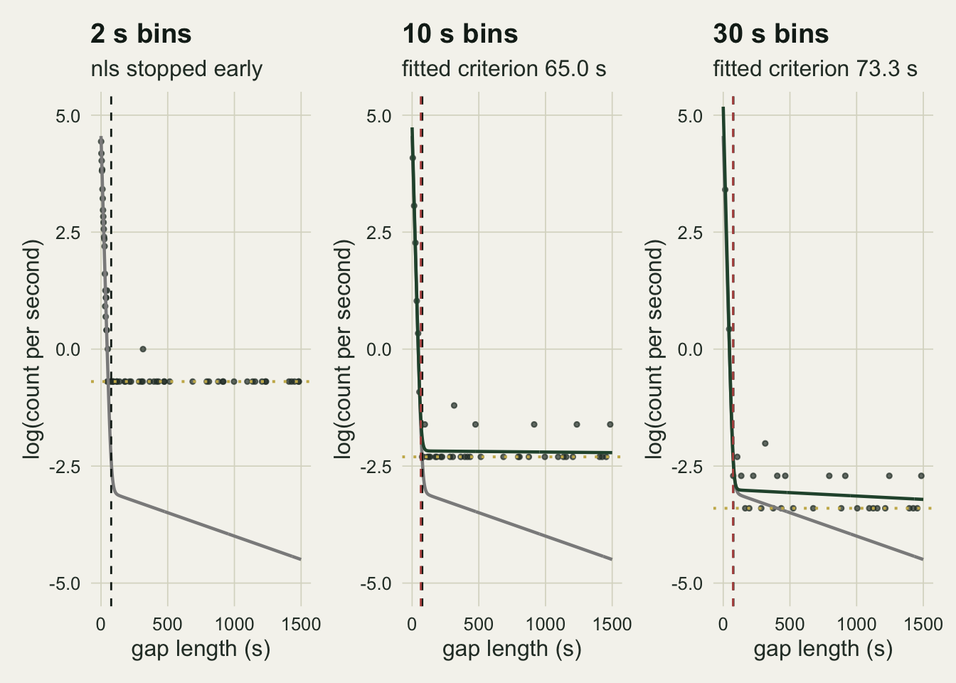
The bin width moves the criterion
set.seed(3190)
R_main <- 150
main <- do.call(rbind, lapply(ratios, function(ratio) {
  s_bt <- f_in / ratio; crit_true <- bec(p_in, f_in, s_bt)
  do.call(rbind, lapply(seq_len(R_main), function(i) {
    g  <- sim_gaps(n_gap, p_in, f_in, s_bt)
    nl <- sapply(bins, function(w) nls_bec(g$x, w))
    crits <- c(truth = crit_true, ml = ml_exp2(g$x), lsurv = lsurv_break(g$x),
               setNames(nl["crit", ], paste0("nls_", bins)),
               setNames(sapply(bins, function(w) pois_bec(g$x, w)), paste0("pois_", bins)))
    data.frame(ratio = ratio, rep = i, method = names(crits), crit = unname(crits),
               rel = unname(crits) / crit_true,
               degenerate = c(NA, NA, NA, nl["slow_mean", ] > 10 * ratio / f_in, NA, NA, NA),
               mis = sapply(crits, function(cc) if (is.na(cc)) NA else mis_share(g$x, g$within, cc)),
               bouts = sapply(crits, function(cc) if (is.na(cc)) NA else bout_err(g$x, g$within, cc)))
  }))
}))

by_cell <- function(v, fun) tapply(v, list(main$method, main$ratio), fun)
rel_med   <- by_cell(main$rel, function(v) median(v, na.rm = TRUE))
fail_tab  <- by_cell(main$crit, function(v) mean(is.na(v)))
degen_tab <- by_cell(main$degenerate, function(v) if (all(is.na(v))) NA else mean(v, na.rm = TRUE))
abs_med   <- by_cell(abs(main$rel - 1), function(v) median(v, na.rm = TRUE))
mis_med   <- by_cell(main$mis, function(v) median(v, na.rm = TRUE))
bout_med  <- by_cell(main$bouts, function(v) median(v, na.rm = TRUE))
fail_se_max <- sqrt(0.25 / R_main)
nls_rows <- paste0("nls_", bins); lik_rows <- c("ml", paste0("pois_", bins))
The main grid repeats that for 150 animals at each rate ratio, with 1000 gaps each, and fits every animal by every method. Each animal is binned at all three widths, so the bin-width comparison is paired.
The least squares fit on log counts gives median ratios of estimated to true criterion of 0.76, 1.04 and 1.23 at 2, 10 and 30 s bins when the rate ratio is 20; 0.62, 0.84 and 1.04 at a ratio of 100; and 0.52, 0.71 and 0.87 at 500. Wider bins give longer criteria in every row, which is the direction Luque and Guinet (2007) reported for sequential differences analysis, a related histogram method, and no single width is close to the truth at all three ratios. These medians cover only the fits that nls() returned. With its default settings it stopped with an error at 2 s bins in 27.3, 18.0 and 0.7 per cent of animals at the three ratios, and at 10 s in 0.7, 2.7 and 0.0 per cent. With 150 animals per cell the Monte Carlo standard error of such a share is at most 0.041. The section after the next figure shows what the stopped fits were heading for.
Call a fit degenerate when its slow component has a mean gap more than ten times the true one. Among the 2 s fits that were returned, the degenerate share is 0.96, 1.00 and 1.00; at 10 s it is 0.34, 0.95 and 1.00; at 30 s 0.01, 0.37 and 1.00. A returned histogram fit that reports a criterion has, in most cells of this grid, no slow process in it at all.
The two likelihood fits do not move. Maximum likelihood on the raw gaps gives medians of 0.996, 0.999 and 1.002, and the Poisson likelihood of the very histograms the least squares fit used gives medians between 0.994 and 1.008 over all nine combinations of bin width and ratio. For a single animal the typical error is larger than the median suggests: the median absolute relative error is 2.5 to 4.7 per cent for the likelihood fits, against 48.1 per cent in the worst least squares cell. So binning the gaps is not what breaks the histogram method. The Poisson fit keeps the empty bins and uses each bin’s exact probability; the least squares fit drops the empty bins, takes logs and treats the midpoint as the whole bin.
lab_map <- c(nls_2 = "NLS 2 s", nls_10 = "NLS 10 s", nls_30 = "NLS 30 s",
             pois_2 = "Poisson 2 s", pois_10 = "Poisson 10 s", pois_30 = "Poisson 30 s", ml = "ML gaps")
plot_main <- main[main$method %in% names(lab_map) & !is.na(main$rel), ]
plot_main$label  <- factor(lab_map[plot_main$method], levels = lab_map)
plot_main$family <- ifelse(grepl("nls", plot_main$method), "least squares on log counts", "likelihood")
plot_main$ratio_lab <- factor(paste("rate ratio", plot_main$ratio), levels = paste("rate ratio", ratios))
ggplot(plot_main, aes(label, rel, fill = family)) +
  geom_hline(yintercept = 1, colour = te_ink, linewidth = 0.4) +
  geom_boxplot(outlier.size = 0.6, outlier.colour = te_body, linewidth = 0.35, width = 0.7) +
  facet_wrap(~ ratio_lab, ncol = 1) +
  scale_fill_manual(values = c("least squares on log counts" = te_rust, "likelihood" = te_forest), name = NULL) +
  coord_cartesian(ylim = c(0.2, 1.8)) +
  labs(x = NULL, y = "estimated / true criterion",
       title = "The histogram fit follows the bin width",
       subtitle = "nls fits that stopped with an error are left out of the least squares boxes") +
  theme_datasheet() +
  theme(legend.position = "bottom")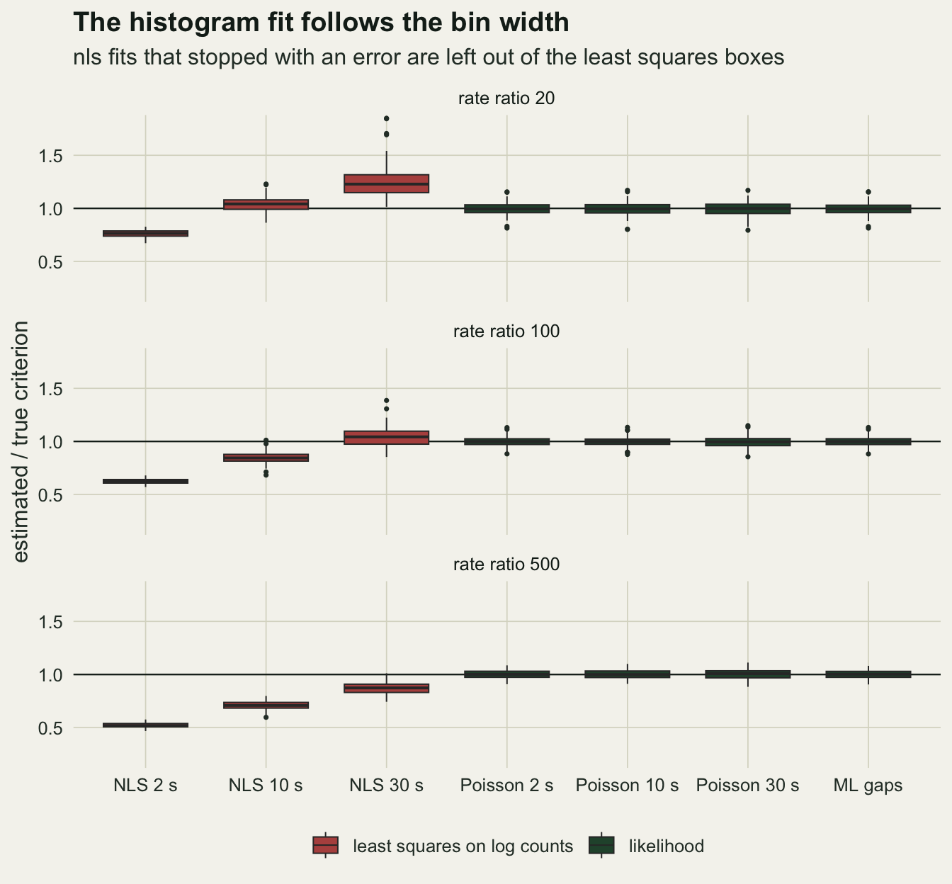
Stopped fits head for the floor
set.seed(3191)
n_check <- 60
s_check <- f_in / 100
crit_check <- bec(p_in, f_in, s_check)
chk <- t(replicate(n_check, {
  g <- sim_gaps(n_gap, p_in, f_in, s_check)
  capped <- nls_bec(g$x, 2, warn_only = TRUE)
  c(default = nls_bec(g$x, 2)[["crit"]] / crit_check,
    capped = capped[["crit"]] / crit_check, slow_mean = capped[["slow_mean"]],
    rss_fit = capped[["rss"]], rss_true = rss_true_log(g$x, 2, p_in, f_in, s_check))
}))
stopped <- is.na(chk[, "default"])
chk_fail_default <- mean(stopped)
chk_fail_capped  <- mean(is.na(chk[, "capped"]))
chk_med_default  <- median(chk[!stopped, "default"])
chk_med_all      <- median(chk[, "capped"])
chk_med_stopped  <- median(chk[stopped, "capped"])
chk_slow_stopped <- range(chk[stopped, "slow_mean"])
chk_rss_below    <- sum(chk[, "rss_fit"] < chk[, "rss_true"])
chk_rss_share    <- max(chk[, "rss_fit"] / chk[, "rss_true"])

floor_crit <- function(n, p, f, w) log(n * p * f * w) / f
floor_rel <- outer(bins, ratios, function(w, r) floor_crit(n_gap, p_in, f_in, w) / bec(p_in, f_in, f_in / r))
floor_mask <- degen_tab[nls_rows, ] >= 0.9
floor_over <- (floor_rel / rel_med[nls_rows, ])[floor_mask]
floor_above <- sum(floor_over > 1)
The error that stops nls() on the animal in figure 1 reads “function evaluation limit reached without convergence”. The chunk above simulates 60 new animals at a rate ratio of 100 and fits each 2 s histogram twice: with the default settings, and with warnOnly = TRUE in nls.control(), which makes nls() return the parameters where it stopped instead of an error. The default fit stopped on 17 per cent of the animals and the warnOnly fit on 0 per cent. Among the animals whose default fit stopped, the returned fits have a median criterion ratio of 0.641 and a slow component with a mean gap between 0.86 and 3.11 million s, against a true 1000 s. The fits that finished normally have a median of 0.621, and all 60 returned fits together 0.624.
The stopped fits are the same fit as the degenerate ones. nls() runs out of function evaluations while the slow rate is still sliding towards zero; allowed to return where it stopped, it gives the floor criterion like the fits that did finish. How many animals fail is therefore a property of the software settings, and leaving them out of a median changes little, as the two medians above show. The floor is a property of the method: on its own 2 s histogram, the returned fit had a smaller residual sum of squares than the true curve in 60 of 60 animals, and never more than 1.4 per cent of it. A least squares optimiser that works well moves away from the truth.
What the fit heads for follows from the floor in figure 1. If every kept bin in the tail holds one gap, the tail is a flat line at log(1/w) for a bin width w. The best two-exponential curve through that is a fast exponential of height n p f meeting a slow component with a rate near zero, and the criterion formula then returns the point where the fast curve meets the floor: n p f exp(-f t) = 1/w, or
t = log(n p f w) / f.
This criterion contains the sample size, the within-bout process and the bin width, and nothing about the between-bout gaps. Divided by the true criterion it gives 0.84, 0.69 and 0.57 at 2 s bins for the three ratios, against observed medians of 0.76, 0.62 and 0.52. Over the cells where at least nine in ten returned fits were degenerate, the floor formula is above the observed median in 5 of 6 cells, by at most 10.6 per cent, and never below it by more than 0.8 per cent. The formula counts every kept bin as a single gap; kept bins holding two or more gaps raise the tail the regression sees, which is a likely reason the fitted criteria come out a little earlier. The formula also predicts the next section: more gaps per animal lengthen the histogram criterion even when the animal’s behaviour is unchanged.
Keeping the empty bins
set.seed(3192)
R_zero <- 100
zero <- do.call(rbind, lapply(seq_len(R_zero), function(i) {
  g <- sim_gaps(n_gap, p_in, f_in, f_in / 100)
  data.frame(w = bins, rel = sapply(bins, function(w) nls_bec(g$x, w, "half")[["crit"]]) /
               bec(p_in, f_in, f_in / 100))
}))
half_med  <- tapply(zero$rel, zero$w, median, na.rm = TRUE)
half_fail <- tapply(is.na(zero$rel), zero$w, mean)
floor_half <- log(2 * n_gap * p_in * f_in * bins) / f_in / bec(p_in, f_in, f_in / 100)
A log of zero can be avoided without dropping the bin, by adding half a count to every bin before taking logs. Refitting 100 new animals at a rate ratio of 100 that way gives medians of 0.74, 0.97 and 1.11 at 2, 10 and 30 s bins, and nls() stopped on none of them. Keeping the zeros removed the stopped fits here but not the bias. The patched empty bins form a floor of their own, at log(0.5/w) instead of log(1/w), and the floor formula with half a gap per bin, log(2 n p f w) / f, gives 0.78, 0.99 and 1.13 of the true criterion against these medians.
The implementation question therefore has a split answer. Dropping empty bins makes the tail flat at log(1/w), and a flat tail is what drives the slow rate towards zero; the least squares fit on log counts, with empty bins dropped or patched, still depends on the bin width; and a fit that treats the same counts as counts, the Poisson likelihood of the main grid, has no bin-width problem at 2, 10 or 30 s. The method is biased as a regression on logs, not as a use of a histogram.
More gaps, a longer criterion
set.seed(3193)
R_n <- 60
design_n <- expand.grid(n = c(200, 1000, 5000), p = c(0.8, 0.95))
size_rows <- do.call(rbind, lapply(seq_len(nrow(design_n)), function(k) {
  n <- design_n$n[k]; p <- design_n$p[k]; s_bt <- f_in / 100; tr <- bec(p, f_in, s_bt)
  do.call(rbind, lapply(seq_len(R_n), function(i) {
    g <- sim_gaps(n, p, f_in, s_bt)
    nl <- sapply(bins, function(w) nls_bec(g$x, w))
    data.frame(n = n, p = p, method = c("ml", paste0("nls_", bins)),
               rel = c(ml_exp2(g$x), nl["crit", ]) / tr)
  }))
}))
size_med  <- aggregate(rel ~ n + p + method, size_rows, median, na.action = na.omit)
size_fail <- aggregate(cbind(fail = is.na(rel)) ~ n + p + method, size_rows, mean, na.action = na.pass)
size_med  <- merge(size_med, size_fail)
sm <- function(n, p, m, col = "rel") size_med[size_med$n == n & size_med$p == p & size_med$method == m, col]
ml_size_range <- range(size_med$rel[size_med$method == "ml"])
The floor formula says the histogram criterion should grow with the logarithm of the number of gaps. The chunk above checks that at a rate ratio of 100 for 200, 1000 and 5000 gaps per animal and two within-bout shares, 60 animals per cell.
With a within-bout share of 0.95 and 10 s bins the median ratio goes from 0.62 at 200 gaps to 0.85 at 1000 and 1.06 at 5000. At 2 s bins it goes from 0.39 to 0.85, and at 30 s from 0.85 to 1.19. With a share of 0.8 the same 10 s fit goes from 0.78 to 1.21. A bin width that happens to be right for one record length is wrong for a longer or shorter one, so a histogram criterion fitted separately per animal will differ between a bird with a long record and one with a short record for no behavioural reason.
At 200 gaps and a share of 0.95 the default nls() stopped in 17, 12 and 32 per cent of animals at the three bin widths, fits that head for the same floor. The likelihood fit to the gaps gave medians between 0.978 and 1.011 across all six cells. Langton, Collett and Sibly (1995) found that the sample size the likelihood method needs depends on the rate ratio and the mixing proportion; figure 3 shows that the histogram method needs something no sample size gives it, a bin width that matches the record.
size_plot <- size_med
size_plot$label <- factor(c(ml = "ML gaps", nls_2 = "NLS 2 s", nls_10 = "NLS 10 s", nls_30 = "NLS 30 s")[size_plot$method],
                          levels = c("NLS 2 s", "NLS 10 s", "NLS 30 s", "ML gaps"))
size_plot$p_lab <- factor(paste("within-bout share", size_plot$p))
ggplot(size_plot, aes(n, rel, colour = label)) +
  geom_hline(yintercept = 1, colour = te_line, linewidth = 0.8) +
  geom_line(linewidth = 0.9) +
  geom_point(size = 2) +
  facet_wrap(~ p_lab) +
  scale_x_log10(breaks = c(200, 1000, 5000)) +
  scale_colour_manual(values = c("NLS 2 s" = te_rust, "NLS 10 s" = te_gold, "NLS 30 s" = te_forest, "ML gaps" = te_ink),
                      name = NULL) +
  labs(x = "gaps per animal", y = "median estimated / true criterion",
       title = "No single bin width is right for every record") +
  theme_datasheet() +
  theme(legend.position = "bottom")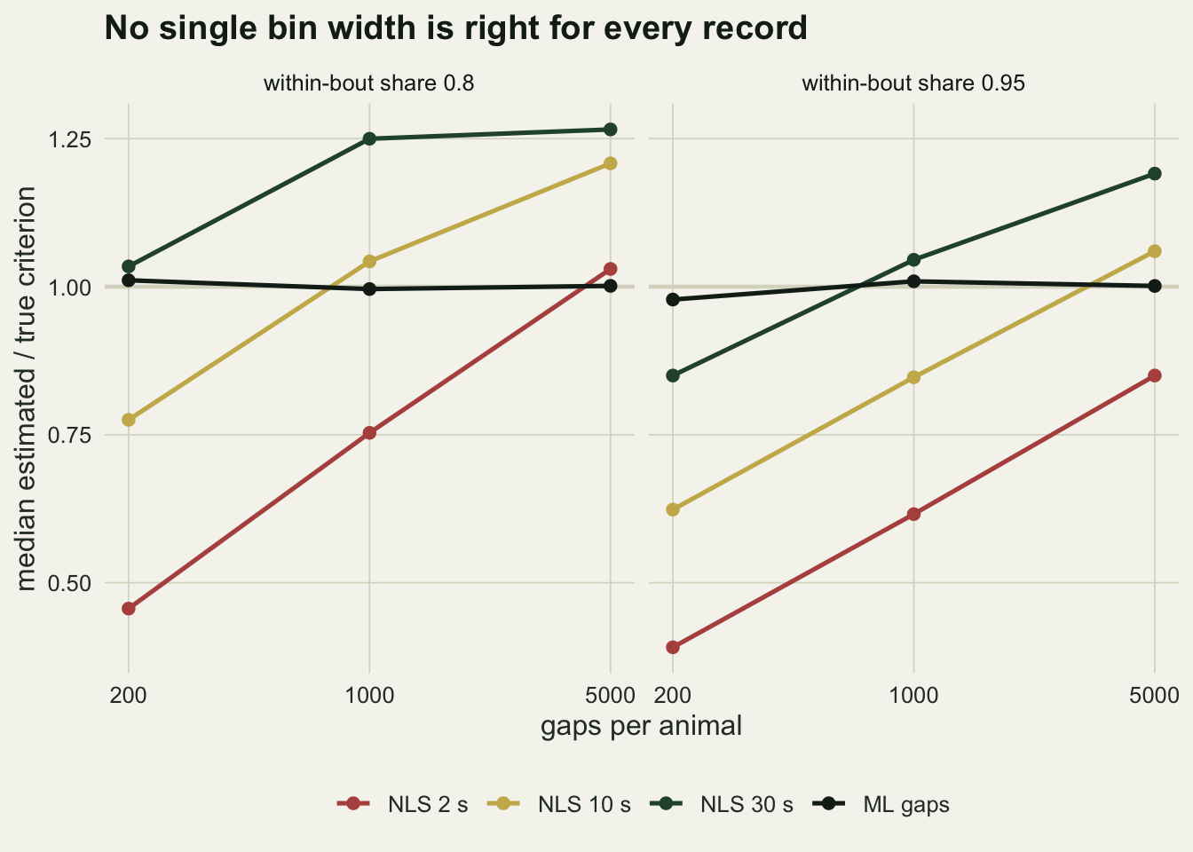
What the criterion does to the bout count
A criterion is a means to a bout count, so the useful question is what these ratios do to the number of bouts. The main grid recorded, for every animal and method, the share of gaps put in the wrong class and the relative error in the number of between-bout gaps, which is the number of bouts minus one.
At a rate ratio of 100 the true criterion misassigns a median 0.40 per cent of gaps and the 2 s histogram criterion 1.00 per cent. Those shares look small because 95 per cent of gaps are short, and even the median 2 s criterion leaves only 0.9 per cent of within-bout gaps beyond it. The bout count shows the difference: a median error of -5.9 per cent with the true criterion, -5.9 with the likelihood fit and 11.5 with the 2 s histogram fit. At a ratio of 500 the 2 s fit overcounts by 14.8 per cent where the true criterion is 1.8 per cent low.
A biased criterion can also look better than the truth. At a ratio of 20 the true criterion undercounts bouts by 23.1 per cent, because many between-bout gaps are shorter than it, while the too-short 2 s criterion lets within-bout gaps start spurious bouts that make up part of the shortfall, and its median error is -5.0 per cent. That is two errors cancelling in one summary; the misassigned share, 1.90 per cent against 1.50, shows that more gaps are in the wrong class.
The two-line break point on the log-survivorship curve lands well short of the criterion: medians of 0.57, 0.45 and 0.38 of the truth, bout counts too high by 36, 55 and 57 per cent. The break of a least squares two-line fit is where the curve bends, which is where the fast process starts to fade, and the misassignment-minimising point lies further out, where the few remaining within-bout gaps are outnumbered by between-bout ones. The break answers a different question, and figure 4 shows what the answer costs if it is used as a criterion.
bout_map <- c(truth = "true criterion", ml = "ML gaps", nls_2 = "NLS 2 s", nls_10 = "NLS 10 s",
              nls_30 = "NLS 30 s", lsurv = "log-survivorship break")
bout_plot <- main[main$method %in% names(bout_map) & !is.na(main$bouts), ]
bout_plot$label <- factor(bout_map[bout_plot$method], levels = rev(bout_map))
bout_plot$ratio_lab <- factor(paste("rate ratio", bout_plot$ratio), levels = paste("rate ratio", ratios))
ggplot(bout_plot, aes(bouts, label)) +
  geom_vline(xintercept = 0, colour = te_ink, linewidth = 0.4) +
  geom_boxplot(fill = te_gold, colour = te_body, outlier.size = 0.5, linewidth = 0.35, width = 0.6) +
  facet_wrap(~ ratio_lab, ncol = 3) +
  scale_x_continuous(labels = function(v) paste0(100 * v, "%")) +
  labs(x = "relative error in the number of bouts", y = NULL,
       title = "The threshold decides the bout count") +
  theme_datasheet() +
  theme(plot.title.position = "plot")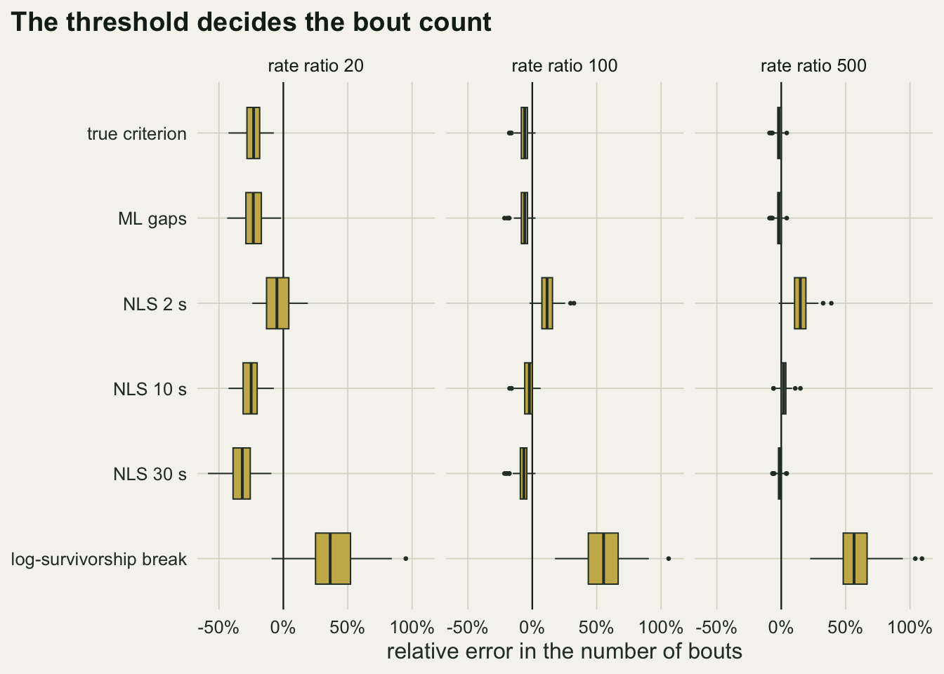
When the gaps are not exponential
set.seed(3194)
R_ln <- 100
s_ln <- f_in / 100
designs_ln <- data.frame(arm = c("a", "b", "c"), sd_in = c(0.5, 1, 1),
                         between = c("exponential", "exponential", "lognormal"), sd_bt = c(NA, NA, 1))
min_crit <- function(mis_fun) {
  tgrid <- seq(1, 3000, by = 1); t0 <- tgrid[which.min(mis_fun(tgrid))]
  optimize(mis_fun, c(max(t0 - 5, 0.01), t0 + 5))$minimum
}
ml_lnexp <- function(x) {
  nll <- function(th) {
    p <- plogis(th[1]); s <- exp(th[4])
    -sum(log(p * dlnorm(x, th[2], exp(th[3])) + (1 - p) * s * exp(-s * x)))
  }
  short <- x[x < quantile(x, 0.9)]
  o <- optim(c(qlogis(0.9), mean(log(short)), log(sd(log(short))),
               log(1 / mean(x[x > quantile(x, 0.95)]))), nll, method = "BFGS")
  p <- plogis(o$par[1]); ml <- o$par[2]; sl <- exp(o$par[3]); s <- exp(o$par[4])
  optimize(function(tc) p * plnorm(tc, ml, sl, lower.tail = FALSE) + (1 - p) * pexp(tc, s),
           c(1, 3000))$minimum
}
ml_lnln <- function(x) {
  lx <- log(x)
  nll <- function(th) {
    p <- plogis(th[1])
    -sum(log(p * dnorm(lx, th[2], exp(th[3])) + (1 - p) * dnorm(lx, th[4], exp(th[5]))))
  }
  lo <- lx[lx < quantile(lx, 0.9)]; hi <- lx[lx > quantile(lx, 0.97)]
  o <- optim(c(qlogis(0.9), mean(lo), log(sd(lo)), mean(hi), log(sd(hi))), nll, method = "BFGS")
  p <- plogis(o$par[1]); mu <- o$par[c(2, 4)]; sg <- exp(o$par[c(3, 5)])
  if (mu[1] > mu[2]) { p <- 1 - p; mu <- rev(mu); sg <- rev(sg) }
  min_crit(function(tc) p * plnorm(tc, mu[1], sg[1], lower.tail = FALSE) + (1 - p) * plnorm(tc, mu[2], sg[2]))
}
between_cdf <- function(tc, k) if (designs_ln$between[k] == "exponential") pexp(tc, s_ln) else
  plnorm(tc, log(1 / s_ln) - designs_ln$sd_bt[k]^2 / 2, designs_ln$sd_bt[k])
ln_truth <- sapply(seq_len(nrow(designs_ln)), function(k) {
  sdl <- designs_ln$sd_in[k]; mu_l <- log(10) - sdl^2 / 2
  min_crit(function(tc) p_in * plnorm(tc, mu_l, sdl, lower.tail = FALSE) + (1 - p_in) * between_cdf(tc, k))
})
ln_rows <- do.call(rbind, lapply(seq_len(nrow(designs_ln)), function(k) {
  sdl <- designs_ln$sd_in[k]; mu_l <- log(10) - sdl^2 / 2; tr <- ln_truth[k]
  do.call(rbind, lapply(seq_len(R_ln), function(i) {
    within <- runif(n_gap) < p_in
    fast_gaps <- rlnorm(n_gap, mu_l, sdl)
    slow_gaps <- if (designs_ln$between[k] == "exponential") rexp(n_gap, s_ln) else
      rlnorm(n_gap, log(1 / s_ln) - designs_ln$sd_bt[k]^2 / 2, designs_ln$sd_bt[k])
    x <- ifelse(within, fast_gaps, slow_gaps)
    crits <- c(truth = tr, ml_exp2 = ml_exp2(x), ml_lnexp = ml_lnexp(x), ml_lnln = ml_lnln(x),
               nls_10 = nls_bec(x, 10)[["crit"]], pois_10 = pois_bec(x, 10))
    data.frame(arm = designs_ln$arm[k], method = names(crits), rel = crits / tr,
               mis = sapply(crits, function(cc) if (is.na(cc)) NA else mis_share(x, within, cc)),
               bouts = sapply(crits, function(cc) if (is.na(cc)) NA else bout_err(x, within, cc)))
  }))
}))
ln_cell <- function(v, fun) tapply(v, list(ln_rows$method, ln_rows$arm), fun)
ln_rel  <- ln_cell(ln_rows$rel, function(v) median(v, na.rm = TRUE))
ln_mis  <- ln_cell(ln_rows$mis, function(v) median(v, na.rm = TRUE))
ln_bout <- ln_cell(ln_rows$bouts, function(v) median(v, na.rm = TRUE))
ln_fail <- ln_cell(ln_rows$rel, function(v) mean(is.na(v)))
Every fit so far assumed the right model. Tolkamp and Kyriazakis (1999) fitted mixtures of normal distributions to log-transformed intervals, which makes both processes lognormal. The chunk above tries three designs, fixed before running, all with a within-bout mean gap of 10 s and a between-bout mean gap of 1000 s. In the first two only the within-bout shape changes: within-bout gaps are lognormal with a log standard deviation of 0.5 or 1, and between-bout gaps stay exponential. In the third both processes are lognormal with a log standard deviation of 1, the form of their model. The truth is defined as before, as the gap length that minimises misassignment under the densities that generated the data, found numerically: 48.4, 114.2 and 115.0 s for the three designs. Each animal is fitted by the two-exponential likelihood, Poisson and least squares fits at 10 s bins, a lognormal plus exponential likelihood and a two-lognormal likelihood.
With only the within-bout shape wrong, the two-exponential likelihood, exact under its own model, misses in both directions: medians of 1.61 and 0.60 of the truth. The direction is consistent with the tail of the within-bout gaps. Over the range where the criterion falls, a lognormal with a log SD of 0.5 has a thinner tail than an exponential of the same mean, so the fitted fast exponential reaches further out than the real gaps do and the criterion is pushed late; with a log SD of 1 the tail is heavier, long within-bout gaps are absorbed into the slow component, and the criterion comes early. The Poisson fit to 10 s bins follows the same pattern (1.41 and 0.59), since it is the same model. The least squares fit gives 0.93 and 0.63; its nearness to the truth at a log SD of 0.5 is its floor bias and the model error pulling in opposite directions, not a sign that it copes with the wrong shape. The lognormal plus exponential likelihood recovers 1.001 and 0.992, while the two-lognormal likelihood, wrong here about the between-bout gaps, gives 1.13 and 1.18.
With both processes lognormal the two-exponential likelihood gives 0.58 of the truth, the Poisson fit 0.56 and the least squares fit 0.60. The lognormal plus exponential likelihood, now wrong about the between-bout gaps, gives 0.959, and the two-lognormal likelihood 0.998.
The misassigned share moves less than the criterion ratios suggest, because the misassignment curve is shallow around its minimum. With a within-bout log SD of 1 and exponential between-bout gaps, the two-exponential likelihood misassigns 1.00 per cent of gaps against 0.70 at the true criterion. The bout count moves more: its median error goes from -8.3 per cent at the truth to 7.1 per cent, and with both processes lognormal from -2.2 to 13.0 per cent. Checking the shapes is worth doing before trusting any criterion, and a likelihood fit makes that check possible, because models with different shapes can be compared on the same gaps.
ln_map <- c(ml_exp2 = "two-exponential ML", pois_10 = "two-exponential Poisson 10 s",
            nls_10 = "two-exponential NLS 10 s", ml_lnexp = "lognormal plus exponential ML",
            ml_lnln = "two-lognormal ML")
arm_map <- c(a = "within log SD 0.5, between exponential", b = "within log SD 1, between exponential",
             c = "within and between lognormal, log SD 1")
ln_plot <- ln_rows[ln_rows$method %in% names(ln_map) & !is.na(ln_rows$rel), ]
ln_plot$label <- factor(ln_map[ln_plot$method], levels = rev(ln_map))
ln_plot$arm_lab <- factor(arm_map[ln_plot$arm], levels = arm_map)
ggplot(ln_plot, aes(rel, label)) +
  geom_vline(xintercept = 1, colour = te_ink, linewidth = 0.4) +
  geom_boxplot(fill = te_forest, colour = te_body, alpha = 0.55, outlier.size = 0.5, linewidth = 0.35, width = 0.6) +
  facet_wrap(~ arm_lab, ncol = 1) +
  scale_x_log10(breaks = c(0.5, 0.7, 1, 1.4, 2)) +
  labs(x = "estimated / true criterion (log scale)", y = NULL,
       title = "A wrong shape moves the likelihood too") +
  theme_datasheet() +
  theme(plot.title.position = "plot")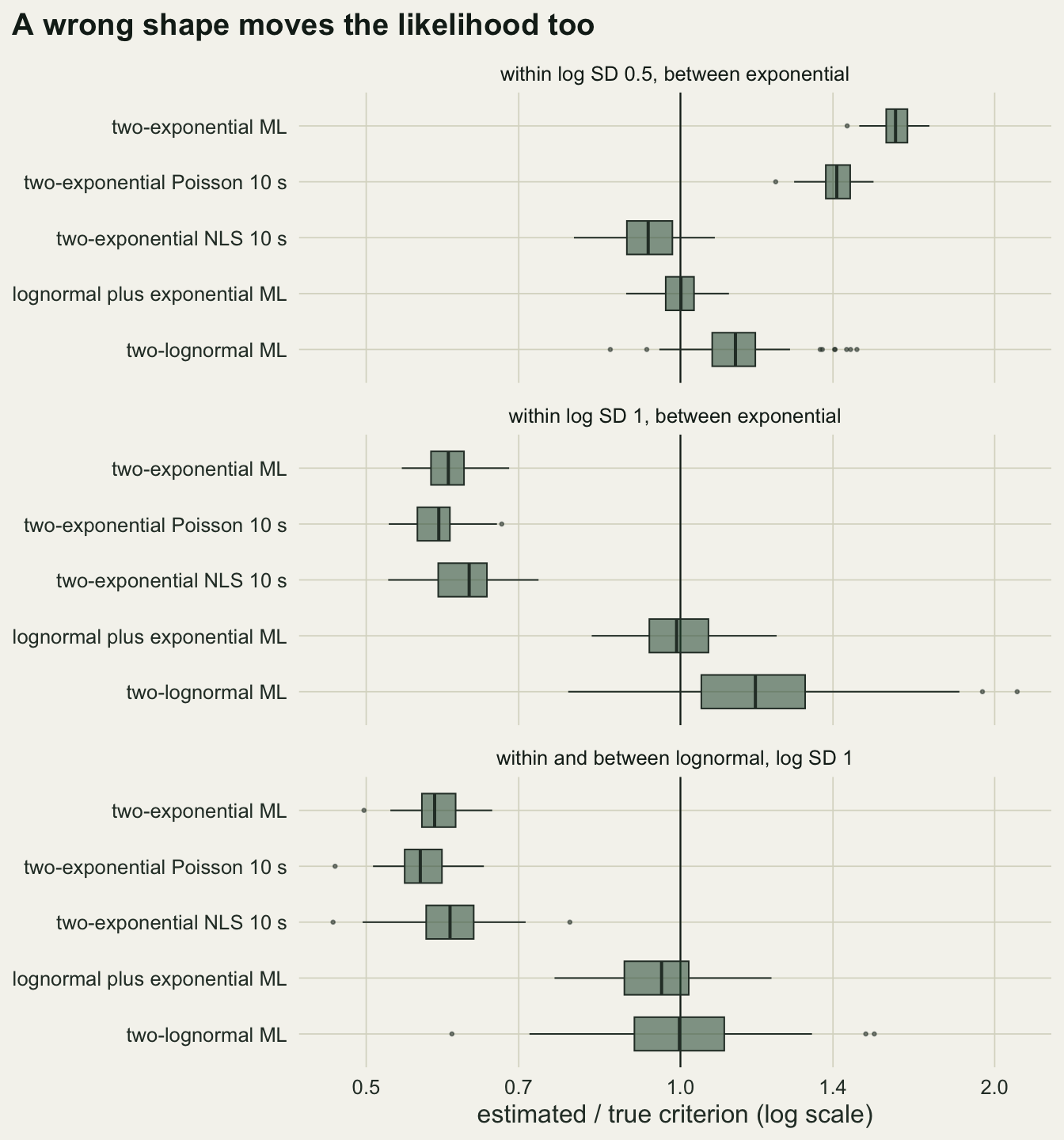
What to report
Name the criterion rule. The misassignment-minimising criterion and the equal-numbers criterion given near the top differed by 18.1 s at a rate ratio of 100 in this design, a larger gap than several of the estimation errors above.
Fit the mixture by maximum likelihood to the gaps, not by regression on a log histogram. If a histogram is all that is available, fit it as counts with a Poisson likelihood that keeps the empty bins. Report the fitted within-bout share, both rates and the criterion, so a reader can recompute the criterion under another rule.
If a published histogram criterion is being reused or compared, report its bin width and the number of gaps it came from. The floor formula, log(n p f w) / f, tells a reader whether the histogram criterion could have been set by the floor rather than by the between-bout gaps: if it is close to the reported criterion, the criterion says little about the slow process.
When criteria are compared across animals or seasons, fit them with the same method, and for the histogram method keep in mind that animals with longer records get longer criteria. Pooling animals for one criterion avoids that but assumes the same processes in all of them.
Report the model for both processes and how it was checked. Lognormal gaps moved the two-exponential criterion to between 0.58 and 1.61 of the truth in the three designs, and each alternative shape compared by likelihood is a single extra optim() call on the same gaps.
Honest limits
The gaps are independent draws from a fixed mixture. Real gaps can be serially correlated, bout lengths vary with prey and time of day, and the between-bout process of a foraging animal is rarely a single exponential. Any of these changes the true criterion and makes the misassignment rule an approximation for both methods. The comparison here shows how the estimators behave where the model is true, plus three designs with lognormal gaps, and no more.
The least squares fit was run with R’s nls() using the port algorithm, lower bounds on the parameters, a log-rate parameterisation and two fixed pairs of starting values. Other software, weights or starting values, such as those from the broken-stick fit that diveMove’s boutinit() provides, can stop on different animals; they were not tried here. What they would not change is that the flat-tailed fits had a smaller residual sum of squares than the true curve, so the bias belongs to the least squares objective on log counts, not to this optimiser.
Gap lengths are continuous here. Recorders sample depth at fixed intervals and feeder logs round to the second, so real gaps are discrete, and a 2 s bin on 1 s data has a lattice structure not simulated here. The rounding also affects the likelihood fit, which should then use the probability of each recorded value rather than a density.
The log-survivorship break is one automated version of reading the curve. A human reading the knee by eye, or a fit that places the line intersection rather than the break, would give different numbers, and those methods were not compared. The misassignment rule was the only one estimated; the equal-numbers rule appears only in its true values.
The misspecification section used three fixed designs. A between-bout process in which a new bout becomes more likely as time since the last one grows, as expected if satiety wears off between meals, was represented only by one lognormal shape with a log SD of 1, whose chance of ending a pause rises over short pauses and then falls; three-process mixtures were not tried either. The alternative likelihood fits were given the right families among a short list, which a real analysis has to find by comparing candidates.
The grid used 150 animals per rate ratio and 60 per sample-size cell to keep the page quick to render. A stopped-fit share in the sample-size cells carries a Monte Carlo standard error of up to 0.065, and medians of the least squares fit rest on fewer animals wherever fits stopped.
References
Slater PJB, Lester NP 1982 Behaviour 79(2-4):153-161 (10.1163/156853982X00229)
Sibly RM, Nott HMR, Fletcher DJ 1990 Animal Behaviour 39(1):63-69 (10.1016/S0003-3472(05)80726-2)
Langton SD, Collett D, Sibly RM 1995 Behaviour 132(9-10):781-799 (10.1163/156853995X00144)
Tolkamp BJ, Kyriazakis I 1999 Animal Behaviour 57(4):807-817 (10.1006/anbe.1998.1022)
Luque SP, Guinet C 2007 Behaviour 144(11):1315-1332 (10.1163/156853907782418213)