library(ggplot2)
library(patchwork)
library(MASS)

te_paper  <- "#f5f4ee"
te_ink    <- "#16241d"
te_body   <- "#2c3a31"
te_forest <- "#275139"
te_rust   <- "#b5534e"
te_gold   <- "#c9b458"
te_line   <- "#dad9ca"

theme_datasheet <- function() {
  theme_minimal(base_size = 12) +
    theme(plot.background  = element_rect(fill = te_paper, colour = NA),
          panel.background = element_rect(fill = te_paper, colour = NA),
          panel.grid.major = element_line(colour = te_line, linewidth = 0.3),
          panel.grid.minor = element_blank(),
          text             = element_text(colour = te_body),
          plot.title       = element_text(colour = te_ink, face = "bold"),
          plot.subtitle    = element_text(colour = te_body),
          axis.text        = element_text(colour = te_body))
}
state_cols <- c(rest = te_line, walk = te_gold, forage = te_forest, shake = te_rust)Accelerometer windows and short behaviours
R
accelerometry
animal behaviour
classification
MASS
simulation
ecology tutorial
Window length sets a ceiling on which short behaviours accelerometer data can detect. Measuring ODBA, VeDBA and LDA classification in R for animal behaviour.
A red deer hind carries a collar with a tri-axial accelerometer logging at 25 Hz. Three weeks later the collar comes back with three weeks of acceleration on three axes, one value every 40 ms, and the plan is the usual one: cut the record into windows of fixed length, compute a handful of summaries for each window, and let a classifier trained on a few hours of video decide whether each window was resting, walking, foraging with the head down, or one of the short, violent head shakes the hind makes when flies are bad. Out of that comes a time budget, and the time budget is the result that goes in the paper.
The window length is usually chosen in a sentence in the methods: two seconds, or four, or whatever the previous study on the species used. This post treats it as what it is, a modelling decision with a measurable cost. A window is labelled with one behaviour, so any window that contains a change of behaviour is mislabelled for part of its length, and a behaviour whose bouts are short compared with the window can only ever win a window by luck. The question is how much that costs, for which behaviour, and whether the familiar summaries (overall accuracy and the time budget) show the cost at all.
The recording problem is a relative of one this site has covered from the observer’s side. The post on behaviour sequences as Markov chains compares a time sampled record with an act record of the same animal and shows that they give two different transition matrices; there the recording rule changes and the behaviour does not. Here the record is continuous and exact, the rule for labelling a window stays fixed at the majority behaviour, and the only thing that changes is the window length. The frequency summary used below is the periodogram of spectral analysis of population cycles, computed on a few seconds of acceleration instead of decades of counts. And the classifier is scored on a separate simulated record, never on windows drawn from the record it was trained on, because consecutive windows of one animal are exactly the kind of grouped rows that the post on data leakage in model validation measured as the largest leak at its settings.
A synthetic collar with a known ethogram
The generating model has four behaviours. Bout lengths are drawn from a gamma distribution with shape two, with mean lengths of 90 s for rest, 30 s for walking, 60 s for foraging and 4 s for a head shake, and at the end of a bout the next behaviour is drawn from a transition matrix with zeros on the diagonal. Gamma bout lengths make this a semi-Markov chain rather than a Markov chain in the strict sense, which avoids the excess of very short bouts that a geometric (memoryless) distribution would produce.
Each behaviour writes a signature on the three axes. Posture sets the static part: the head is level at rest and during a shake, slightly raised when walking and pitched down by 40 degrees when foraging. Movement sets the dynamic part, a sinusoid at a behaviour specific frequency (stride at 2 Hz, a slower nodding rhythm while foraging, 5 Hz for a shake) with amplitudes that differ by axis; the sideways sway axis moves at half the rhythm of the other two, as a head that swings left and right once for every two up and down beats. Every bout gets its own random amplitude, frequency and posture, and every sample gets sensor noise. All of these constants were set before any classifier was run and none was changed afterwards.
hz <- 25                                            # sampling rate
states <- c("rest", "walk", "forage", "shake")
mean_bout <- c(rest = 90, walk = 30, forage = 60, shake = 4)   # seconds
bout_shape <- 2                                     # gamma shape of bout lengths
trans_p <- rbind(rest   = c(0.0, 0.6, 0.3, 0.1),    # next behaviour after a bout
                 walk   = c(0.3, 0.0, 0.5, 0.2),
                 forage = c(0.2, 0.5, 0.0, 0.3),
                 shake  = c(0.2, 0.3, 0.5, 0.0))
base_freq  <- c(0.8, 2, 1.5, 5)                     # Hz, movement rhythm
base_pitch <- c(0, 10, -40, 0)                      # degrees, head posture
amp_surge  <- c(0.01, 0.25, 0.10, 0.20)             # g, dynamic amplitude by axis
amp_sway   <- c(0.01, 0.08, 0.06, 0.70)
amp_heave  <- c(0.01, 0.35, 0.08, 0.15)
noise_g    <- 0.05                                  # sensor noise, g

sim_record <- function(hours) {
  n_tot <- hours * 3600 * hz
  n_max <- ceiling(n_tot / hz)
  st <- integer(n_max); len <- integer(n_max); cur <- 1L; tot <- 0; nb <- 0L
  while (tot < n_tot) {
    nb <- nb + 1L
    st[nb] <- cur
    len[nb] <- max(1L, round(rgamma(1, bout_shape, bout_shape / mean_bout[cur]) * hz))
    tot <- tot + len[nb]
    cur <- sample.int(4, 1, prob = trans_p[cur, ])
  }
  st <- st[seq_len(nb)]; len <- len[seq_len(nb)]
  amp <- rlnorm(nb, 0, 0.35)                        # bout to bout vigour
  frq <- base_freq[st] * rlnorm(nb, 0, 0.12)
  pos <- base_pitch[st] + rnorm(nb, 0, 8)
  bid <- rep(seq_len(nb), len)[seq_len(n_tot)]
  s   <- st[bid]
  tt  <- (seq_len(n_tot) - 1) / hz
  ph  <- 2 * pi * frq[bid] * tt
  a   <- amp[bid]
  pitch <- (pos[bid] + 3 * sin(2 * pi * 0.1 * tt)) * pi / 180
  list(state = s, bout_id = bid, n_bouts = nb, seconds = n_tot / hz,
       surge = -sin(pitch) + a * amp_surge[s] * sin(ph) + rnorm(n_tot, 0, noise_g),
       sway  = a * amp_sway[s] * sin(ph / 2 + 1) + rnorm(n_tot, 0, noise_g),
       heave = cos(pitch) + a * amp_heave[s] * sin(ph + 1) + rnorm(n_tot, 0, noise_g))
}set.seed(1808)
demo <- sim_record(2)
demo_share <- tabulate(demo$state, 4) / length(demo$state)
bout_state <- demo$state[!duplicated(demo$bout_id)]
bout_len_s <- tabulate(demo$bout_id) / hz
demo_mean_bout <- tapply(bout_len_s, factor(bout_state, levels = 1:4), mean)
demo_n_shake <- sum(bout_state == 4)
demo_cv <- sd(bout_len_s) / mean(bout_len_s) # spread of all bout lengths togetherTwo hours of this hind contain 164 bouts, 30 of them head shakes. The realised mean bout lengths are 77, 31, 63 and 4.2 s for rest, walking, foraging and shaking. Shaking fills 1.7 per cent of the record: a behaviour that is frequent as events and rare as time, which is the kind a time budget handles worst.
first_shake <- which(bout_state == 4 & seq_along(bout_state) > 5)[1]
i0 <- match(first_shake, demo$bout_id) - 30 * hz
idx <- i0:(i0 + 60 * hz - 1)
tsec <- (idx - i0) / hz
trace_long <- data.frame(t = rep(tsec, 3),
                         axis = factor(rep(c("surge", "sway", "heave"), each = length(idx)),
                                       levels = c("surge", "sway", "heave")),
                         g = c(demo$surge[idx], demo$sway[idx], demo$heave[idx]))
runs <- rle(demo$state[idx])
band <- data.frame(xmin = c(0, cumsum(runs$lengths)[-length(runs$lengths)]) / hz,
                   xmax = cumsum(runs$lengths) / hz,
                   behaviour = factor(states[runs$values], levels = states))
win_edges <- ((ceiling((i0 - 1) / (8 * hz)) * 8 * hz + 1) - i0) / hz
win_edges <- seq(win_edges, 60, by = 8)
ggplot() +
  geom_rect(data = band, aes(xmin = xmin, xmax = xmax, ymin = -Inf, ymax = Inf, fill = behaviour),
            alpha = 0.45) +
  geom_vline(xintercept = win_edges, linetype = "dashed", colour = te_body, linewidth = 0.3) +
  geom_line(data = trace_long, aes(t, g), colour = te_ink, linewidth = 0.25) +
  facet_grid(axis ~ ., scales = "free_y") +
  scale_fill_manual(values = state_cols, drop = FALSE) +
  labs(x = "Time (s)", y = "Acceleration (g)", fill = NULL,
       title = "A head shake is shorter than an 8 s window") +
  theme_datasheet() + theme(legend.position = "top")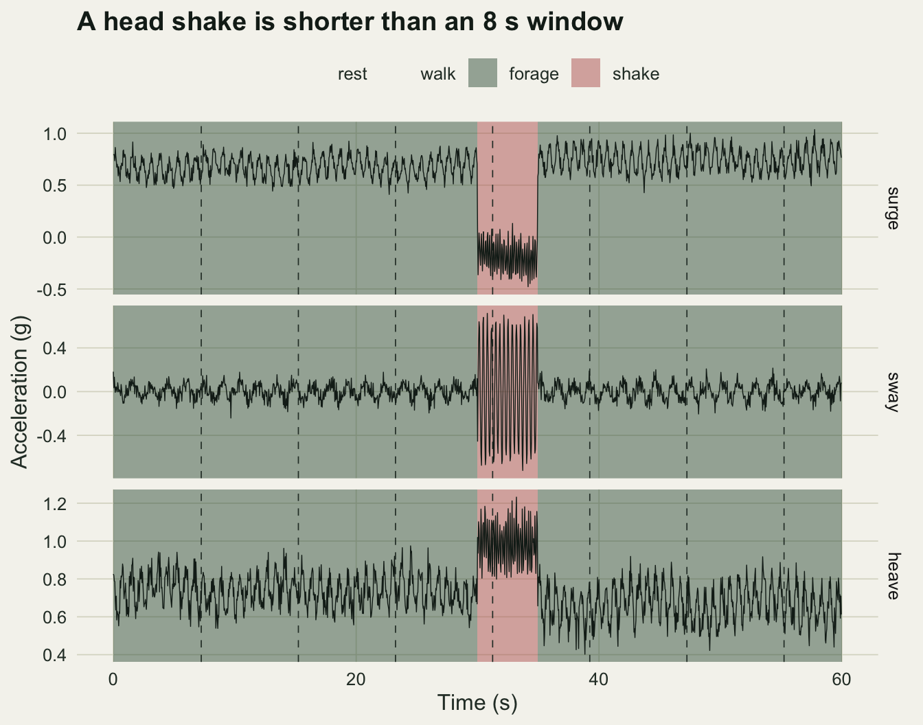
shake_idx <- idx[demo$state[idx] == 4]
win_of <- (shake_idx - 1) %/% (8 * hz)
shake_split <- as.vector(table(win_of)) / hz
trace_bout_s <- length(shake_idx) / hz
The shake in the figure lasts 5.0 s, and the 8 s window grid cuts it into pieces of 1.2 and 3.7 s. Neither piece fills half of its window, so both windows are forage by majority, and a perfect classifier that returned the majority label would record no shaking here at all.
Features per window
Static acceleration, the part that reflects posture, is taken as a centred running mean of each axis over 3 s, computed on the whole record before it is cut into windows, so it does not depend on where the window boundaries fall. Shepard and colleagues 2008 showed that ODBA changes with the length of this running mean and recommend at least 3 s when the dominant stroke period is shorter than that, which holds for the movement rhythms built into this simulation (the slowest, the sideways sway at rest, has a base period of 2.5 s). Dynamic acceleration is what is left after subtracting it. From those come the two standard activity summaries, overall dynamic body acceleration (ODBA, the sum of absolute dynamic values over the three axes, Wilson and colleagues 2006) and vectorial dynamic body acceleration (VeDBA, the length of the dynamic vector, Qasem and colleagues 2012), plus the root mean square of the dynamic signal on each axis, the frequency with the most power in the summed periodogram of the three axes, and the pitch of the mean static vector in the window. Seven features, all of which appear in some form in the feature sets used by Nathan and colleagues 2012.
A common shortcut takes the static part as the mean of each window instead. The function below offers both, and the budget section compares them, because they do not give the same answer.
The window is also given a true label, the behaviour that occupies most of its samples, and a purity, the share of the window that behaviour occupies.
run_mean <- function(v, k) {                         # centred running mean, k samples each side
  cs <- c(0, cumsum(v)); n <- length(v); i <- seq_len(n)
  lo <- pmax(i - k, 1); hi <- pmin(i + k, n)         # shrinks at the two ends of the record
  (cs[hi + 1] - cs[lo]) / (hi - lo + 1)
}
static_s <- 3                                        # seconds of smoothing for static acceleration

window_features <- function(rec, win_s, static = "running") {
  w <- win_s * hz; n_win <- floor(length(rec$state) / w); k <- n_win * w
  as_win <- function(v) matrix(v[seq_len(k)], nrow = w)      # one column per window
  ax <- as_win(rec$surge); ay <- as_win(rec$sway); az <- as_win(rec$heave)
  if (static == "running") {
    h <- floor(static_s * hz / 2)                   # 37 samples each side: 75 samples, 3 s
    sx <- as_win(run_mean(rec$surge, h)); sy <- as_win(run_mean(rec$sway, h))
    sz <- as_win(run_mean(rec$heave, h))
  } else {                                           # shortcut: one static value per window
    sx <- matrix(rep(colMeans(ax), each = w), nrow = w)
    sy <- matrix(rep(colMeans(ay), each = w), nrow = w)
    sz <- matrix(rep(colMeans(az), each = w), nrow = w)
  }
  dx <- ax - sx; dy <- ay - sy; dz <- az - sz
  mx <- colMeans(sx); my <- colMeans(sy); mz <- colMeans(sz)
  pw <- Mod(mvfft(dx))^2 + Mod(mvfft(dy))^2 + Mod(mvfft(dz))^2
  pos_f <- 2:(floor(w / 2) + 1)                      # the zero frequency is left out
  cnt <- vapply(1:4, function(j) colSums(as_win(rec$state) == j), numeric(n_win))
  feat <- data.frame(odba     = colMeans(abs(dx) + abs(dy) + abs(dz)),
                     vedba    = colMeans(sqrt(dx^2 + dy^2 + dz^2)),
                     rms_surge = sqrt(colMeans(dx^2)),
                     rms_sway  = sqrt(colMeans(dy^2)),
                     rms_heave = sqrt(colMeans(dz^2)),
                     dom_freq = max.col(t(pw[pos_f, , drop = FALSE]), "first") * hz / w,
                     pitch    = atan2(-mx, sqrt(my^2 + mz^2)) * 180 / pi)
  feat$label  <- factor(states[max.col(cnt, "first")], levels = states)
  feat$purity <- apply(cnt, 1, max) / w
  list(feat = feat, counts = cnt)
}
demo_f4 <- window_features(demo, 4)$feat
vedba_excess <- max(demo_f4$vedba - demo_f4$odba)
pure4 <- demo_f4[demo_f4$purity == 1, ]
feat_means <- aggregate(cbind(vedba, dom_freq, pitch) ~ label, data = pure4, FUN = median)
Two sanity checks come free. VeDBA can never exceed ODBA, since the length of a vector is at most the sum of the absolute values of its components, and across the 1800 four second windows of the demonstration record the largest value of VeDBA minus ODBA is -0.034. And on pure windows the features separate the behaviours the way the design says they should: median VeDBA of 0.080 g at rest, 0.311 g walking, 0.123 g foraging and 0.574 g shaking; median dominant frequency of 2.00 Hz for walking and 2.50 Hz for shaking, where the peak comes from the large, slower sway axis rather than the 5 Hz rhythm; median pitch of -43 degrees while foraging. The frequency resolution of a window of length W is 1/W Hz, so a one second window can only report whole hertz.
Mixed windows and a ceiling set by bout length
Before any classifier, the window length already decides how much of the record can be labelled correctly. Suppose a classifier returned the majority label of every window without error. Every sample in that window belonging to a minority behaviour would still be wrong. The share of a behaviour’s samples that sit in windows it wins is therefore a ceiling on its recall for any method that gives one label per window.
For a single bout of length L cut by windows of length W at a random offset, that ceiling depends on L and W only through L/W: rescaling time does not change which pieces of the bout fill more than half a window. The next chunk computes it for gamma bouts of shape two by simulation, on a grid of the ratio of mean bout length to window length. It ignores the neighbours of the bout, which matters only when three behaviours share one window.
captured <- function(bout, off, w = 1) {           # bout samples in windows the bout wins
  first <- pmin(bout, w - off)
  rest_len <- pmax(bout - first, 0)
  n_full <- floor(rest_len / w)
  last <- rest_len - n_full * w
  (first > w / 2) * first + n_full * w + (last > w / 2) * last
}
set.seed(2208)
ratio_grid <- 2^seq(-3.5, 7, by = 0.25)
n_bout_mc <- 20000
ceiling_curve <- data.frame(ratio = ratio_grid, recall = vapply(ratio_grid, function(m) {
  bout <- rgamma(n_bout_mc, bout_shape, bout_shape / m)
  sum(captured(bout, runif(n_bout_mc))) / sum(bout)
}, numeric(1)))
ceil_at <- function(m) approx(log2(ceiling_curve$ratio), ceiling_curve$recall, log2(m))$y
ceil_1 <- ceil_at(1); ceil_half <- ceil_at(0.5); ceil_4 <- ceil_at(4); ceil_32 <- ceil_at(32)
For a mean bout exactly as long as the window the ceiling is 0.74. At a ratio of four it is 0.94; at a half it is 0.48; and it takes a ratio of 32 to reach 0.992. The ceiling is not a cliff at a ratio of one but a long shoulder, so even behaviours with bouts several times the window lose a visible share.
To check the curve against the full record, and to have test data for the classifier, the experiment below simulates six independent pairs of twelve hour records. In each pair one record trains the classifier and the other is only used to score it. Six window lengths are compared, from 1 to 32 s, non-overlapping and starting at the first sample.
win_set <- c(1, 2, 4, 8, 16, 32)
n_pair <- 6; rec_hours <- 12

score_pair <- function(train, test, win_s, static) {
  a <- window_features(train, win_s, static); b <- window_features(test, win_s, static)
  fit <- lda(droplevels(label) ~ odba + vedba + rms_surge + rms_sway + rms_heave +
               dom_freq + pitch, data = a$feat)
  pred <- factor(as.character(predict(fit, b$feat)$class), levels = states)
  cnt <- b$counts; tot <- colSums(cnt)
  p_i <- as.integer(pred); l_i <- as.integer(b$feat$label); rows <- seq_len(nrow(cnt))
  hit <- cnt[cbind(rows, p_i)]                     # samples the prediction gets right
  won <- cnt[cbind(rows, l_i)]                     # samples of the window's majority
  by_class <- function(v, g) vapply(1:4, function(j) sum(v[g == j]), numeric(1))
  pred_len <- tabulate(p_i, 4) * win_s * hz        # samples assigned to each behaviour
  prec <- by_class(hit, p_i) / pred_len
  prec[pred_len == 0] <- NA                        # undefined if a behaviour is never called
  c(win = win_s, shortcut = as.numeric(static == "window"),
    win_acc = mean(pred == b$feat$label), samp_acc = sum(hit) / sum(cnt),
    mixed = mean(b$feat$purity < 1),
    poisson = 1 - exp(-win_s * test$n_bouts / test$seconds),
    setNames(by_class(won, l_i) / tot, paste0("orc_", states)),
    setNames(by_class(hit, p_i) / tot, paste0("rec_", states)),
    setNames(prec, paste0("prec_", states)),
    setNames(pred_len / tot, paste0("bud_", states)),
    walk_to_rest = sum(cnt[p_i == 1, 2]) / sum(cnt),   # true walking called rest, share of record
    walk_to_forage = sum(cnt[p_i == 3, 2]) / sum(cnt),
    n_train_shake = sum(a$feat$label == "shake"))
}

res_all <- do.call(rbind, lapply(seq_len(n_pair), function(r) {
  set.seed(3108 + r)                                 # predict() draws random numbers for ties
  train <- sim_record(rec_hours); test <- sim_record(rec_hours)
  do.call(rbind, lapply(c("running", "window"), function(st_method)
    t(sapply(win_set, function(ws) score_pair(train, test, ws, st_method)))))
}))
res_all <- as.data.frame(res_all)
mean_na <- function(v) mean(v, na.rm = TRUE)
se_na   <- function(v) sd(v, na.rm = TRUE) / sqrt(sum(!is.na(v)))
res    <- res_all[res_all$shortcut == 0, ]
res_wm <- res_all[res_all$shortcut == 1, ]
res_mean <- aggregate(. ~ win, data = res, FUN = mean_na, na.action = na.pass)
res_se   <- aggregate(. ~ win, data = res, FUN = se_na, na.action = na.pass)
wm_mean  <- aggregate(. ~ win, data = res_wm, FUN = mean_na, na.action = na.pass)
row_w <- function(ws) which(res_mean$win == ws)
The share of mixed windows is the first thing to compare with arithmetic. If bout ends arrived as a Poisson process, a window of length W would contain at least one with probability one minus exp(-W times the bout rate). At 8 s the simulated share of mixed windows is 0.155 against 0.160 from that formula, and at 32 s 0.492 against 0.503. The formula runs slightly high at both lengths. Bout ends here are not a Poisson process: the record mixes 4 s head shakes with bouts of a minute or more, so bout ends come in close pairs around each shake, and clustered ends fall in fewer windows than the same number of independent ends would. Taken together, the bout lengths of the two hour demonstration record have a coefficient of variation of 1.11, more spread than the exponential lengths of a Poisson process, which have one. (Gamma bouts of shape two on their own would push the share the other way.)
orc_long <- data.frame(win = rep(res_mean$win, 4),
                       behaviour = factor(rep(states, each = nrow(res_mean)), levels = states),
                       recall = unlist(res_mean[paste0("orc_", states)]))
orc_long$ratio <- mean_bout[as.character(orc_long$behaviour)] / orc_long$win
orc_long$curve <- ceil_at(orc_long$ratio)
ceiling_gap <- max(abs(orc_long$recall - orc_long$curve))
shake_orc <- orc_long$recall[orc_long$behaviour == "shake"]
above <- orc_long[order(orc_long$curve - orc_long$recall), ][1:4, ] # furthest above the lineggplot() +
geom_line(data = ceiling_curve, aes(ratio, recall), colour = te_body, linewidth = 0.6) +
geom_point(data = orc_long, aes(ratio, recall, fill = behaviour), shape = 21, size = 3,
colour = te_ink) +
geom_vline(xintercept = 1, linetype = "dashed", colour = te_body, linewidth = 0.3) +
scale_x_log10(breaks = 2^seq(-3, 6, by = 1),
labels = function(b) ifelse(b < 1, paste0("1/", 1 / b), b)) +
scale_fill_manual(values = state_cols) +
labs(x = "Mean bout length / window length", y = "Largest achievable recall",
fill = NULL, title = "One curve for every behaviour") +
theme_datasheet() + theme(legend.position = "top")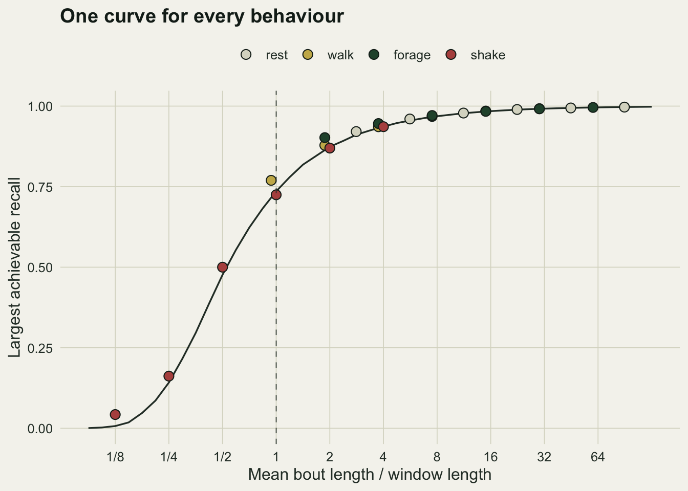
The points from the full records fall on the single-bout line: the largest gap between any of the 24 points and the curve is 0.054. Points below the line miss it by at most 0.011. Of the four points furthest above it, 3 are at 32 s, where a window can hold three behaviours and one of them can win with less than half the samples, which the single-bout calculation does not allow. For the head shake the ceiling is 0.94 at 1 s, 0.50 at 8 s, 0.16 at 16 s and 0.043 at 32 s. Once the ratio of mean bout to window is known, and the bouts are gamma with shape two as here, the ceiling is known, whatever the behaviour and whatever the classifier, provided the classifier is trained to return the majority label and manages it.
What the classifier reports and what it does
Linear discriminant analysis from MASS is fitted to the training windows with their majority labels and asked to label the test windows. It is the plainest classifier there is, which is the point: it is not the classifier that sets the ceiling.
acc_1  <- res_mean$win_acc[row_w(1)];  acc_16 <- res_mean$win_acc[row_w(16)]
sacc_1 <- res_mean$samp_acc[row_w(1)]; sacc_32 <- res_mean$samp_acc[row_w(32)]
acc_32 <- res_mean$win_acc[row_w(32)]
se_acc_max <- max(res_se$win_acc, res_se$samp_acc)
rec_sh <- res_mean$rec_shake; prec_sh <- res_mean$prec_shake; orc_sh <- res_mean$orc_shake
se_rec_sh <- max(res_se$rec_shake)
n_tr_sh_32 <- res$n_train_shake[res$win == 32]
Scored the usual way, as the share of test windows whose predicted label matches the majority label, accuracy is 0.983 at 1 s and 0.948 at 16 s, and still 0.932 at 32 s. Scored per sample, as the share of the twelve hours assigned to the right behaviour, it falls from 0.981 to 0.847. The largest Monte Carlo standard error of either accuracy at any window is 0.003. Both numbers look like a classifier that works, and both are dominated by rest and foraging, which fill most of the record in long bouts.
The head shake tells a different story. Its sample recall, the share of true shaking that ends up inside windows called shake, is 0.84 at 1 s, 0.66 at 4 s, 0.49 at 8 s and 0.09 at 32 s, with Monte Carlo standard errors of at most 0.021.
Up to 8 s the classifier’s recall sits below the majority-label ceiling or level with it (0.50 at 8 s), but at 16 and 32 s it is above it (0.16 and 0.043). This is not a contradiction. The ceiling bounds a method that returns the majority label, and the classifier does not: a window holding a few seconds of violent shaking and a longer stretch of foraging has a VeDBA and a dominant frequency that look like shaking, so it can be called shake even though its majority label is forage. The price is paid in precision, the share of the time called shaking that really is shaking: 0.94 at 1 s, 0.63 at 8 s and 0.40 at 32 s. At the longest window the six training records held 1, 2, 2, 2, 1 and 4 windows labelled shake, so the shake class is fitted to a handful of points and the 32 s values for this behaviour are barely estimates.
shake_long <- data.frame(win = rep(res_mean$win, 2),
                         measure = factor(rep(c("recall", "precision"), each = nrow(res_mean)),
                                          levels = c("recall", "precision")),
                         value = c(rec_sh, prec_sh),
                         se = c(res_se$rec_shake, res_se$prec_shake))
ggplot(shake_long, aes(win, value, colour = measure)) +
  geom_line(data = data.frame(win = res_mean$win, value = orc_sh), aes(win, value),
            inherit.aes = FALSE, linetype = "dashed", colour = te_body, linewidth = 0.5) +
  geom_errorbar(aes(ymin = value - 2 * se, ymax = value + 2 * se), width = 0.08 * log10(2),
                linewidth = 0.4) +
  geom_line(linewidth = 0.8) + geom_point(size = 2.5) +
  annotate("text", x = 16, y = orc_sh[5] - 0.08, label = "majority ceiling", colour = te_body,
           size = 3.5) +
  scale_x_log10(breaks = win_set) +
  scale_colour_manual(values = c(recall = te_rust, precision = te_forest)) +
  coord_cartesian(ylim = c(0, 1)) +
  labs(x = "Window length (s, log scale)", y = "Share", colour = NULL,
       title = "Head shakes: recall and precision fall together") +
  theme_datasheet() + theme(legend.position = "top")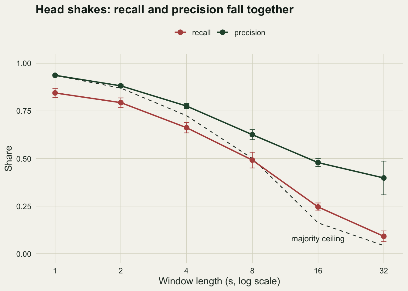
The time budget flatters it
The time budget is computed the way it usually is: count the windows given each label and multiply by the window length. Divided by the true time in each behaviour, a value of one is an unbiased budget.
bud_long <- data.frame(win = rep(res_mean$win, 4),
                       behaviour = factor(rep(states, each = nrow(res_mean)), levels = states),
                       ratio = unlist(res_mean[paste0("bud_", states)]),
                       se = unlist(res_se[paste0("bud_", states)]))
bud_sh <- res_mean$bud_shake; se_bud_sh <- res_se$bud_shake
long_dev <- max(abs(unlist(res_mean[row_w(16), paste0("bud_", states[1:3])]) - 1))
long_dev_32 <- max(abs(unlist(res_mean[row_w(32), paste0("bud_", states[1:3])]) - 1))
bud_wk <- res_mean$bud_walk; bud_rs <- res_mean$bud_rest; bud_fg <- res_mean$bud_forage
set.seed(3200)
true_share <- tabulate(sim_record(rec_hours)$state, 4) / (rec_hours * 3600 * hz) # from one further record
walk_short <- (1 - res_mean$bud_walk) * true_share[2]    # walking lost, share of the record
wtr <- res_mean$walk_to_rest; wtf <- res_mean$walk_to_forage
paired <- function(col) {                                # running mean minus shortcut, per pair
  d <- res[[col]] - res_wm[[col]]
  cbind(mean = tapply(d, res$win, mean), se = tapply(d, res$win, function(v) sd(v) / sqrt(length(v))))
}
d_shake <- paired("bud_shake"); d_walk <- paired("bud_walk"); d_rest <- paired("bud_rest")
At 8 s the estimated time spent shaking is 0.79 of the true time (Monte Carlo standard error 0.04), although the classifier found only 49 per cent of the actual shaking. The budget ratio is recall divided by precision, so false calls in mixed windows make up part of the missed shaking, and the budget falls much more slowly than recall. It has already fallen by 8 s, though, and at 16 s it is 0.51 (standard error 0.02) and at 32 s 0.26 (standard error 0.06). Even at 1 s the head shake budget is 0.90, so the classifier loses some shaking even at the shortest window.
The long behaviours drift too. Walking is estimated at 0.96 of its true time at 1 s and 0.81 at 32 s, rest at 1.02 and 1.08, and foraging at 1.010 and 1.049 (standard errors at most 0.013). As a share of the whole record, the net loss of walking grows from 0.009 at 1 s to 0.038 at 32 s. The true walking that sits inside windows called rest grows from 0.009 to 0.040, and inside windows called foraging from 0.001 to 0.032; these are gross flows, partly offset by rest and foraging called walking, but they show that long windows hand walking time to both of the behaviours that bracket its bouts. In this design the budgets for rest, walking and the head shake are at their best at 1 or 2 s and get worse as the window lengthens, so there is no trade-off between the short and the long behaviours to manage: the shortest windows served all four.
The static component matters here. Scored on the same records with the same classifier, the window-mean shortcut gives nearly the same budgets up to 4 s, where the paired difference in the head shake budget is at most 0.051. From 8 s on it does not. At 8 s the shortcut puts the head shake budget at 0.90, walking at 1.03 and rest at 0.97, against 0.79, 0.92 and 1.04 with the running mean (paired standard errors of the differences at most 0.015). With the shortcut, a change of posture inside a window (the head going from 40 degrees down to level) is counted as dynamic acceleration, and at long windows that moves time out of rest and into walking and shaking. The shortcut’s head shake budget looks better, partly through extra hits but more through extra false calls: at 8 s its precision is 0.58 against 0.63, while its recall is 0.52 against 0.49.
ggplot(bud_long, aes(win, ratio, colour = behaviour)) +
  geom_hline(yintercept = 1, linetype = "dashed", colour = te_body, linewidth = 0.4) +
  geom_errorbar(aes(ymin = ratio - 2 * se, ymax = ratio + 2 * se), width = 0.08 * log10(2),
                linewidth = 0.4, position = position_dodge(width = 0.25 * log10(2))) +
  geom_line(linewidth = 0.7, position = position_dodge(width = 0.25 * log10(2))) +
  geom_point(size = 2.3, position = position_dodge(width = 0.25 * log10(2))) +
  scale_x_log10(breaks = win_set) +
  scale_colour_manual(values = c(rest = "#8a8a78", walk = te_gold, forage = te_forest,
                                 shake = te_rust)) +
  labs(x = "Window length (s, log scale)", y = "Estimated / true time", colour = NULL,
       title = "Budgets drift as the window lengthens") +
  theme_datasheet() + theme(legend.position = "top")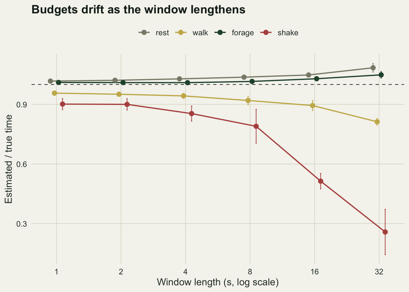
What to report
Give the window length together with the mean bout length of every behaviour that matters to the question, and state the ratio. The figure of the ceiling turns that ratio into the largest share of a behaviour that a one-label-per-window method can recover; readers whose bout lengths are roughly gamma shaped can place a study on the curve. For other bout length distributions the captured() function takes any vector of bout lengths, in units of the window, with random offsets.
Report recall and precision per behaviour, computed per sample of time rather than per window, and on records from animals or days that the classifier never saw. Overall window accuracy is the wrong summary for a rare, short behaviour: here it never fell below 0.932 at any window length, while head shake recall fell to 0.09.
If the result is a time budget, do not treat a good budget for a short behaviour as evidence that the behaviour was detected. At 8 s the shaking budget was 0.79 of the truth while only 49 per cent of the shaking was found, because false calls in mixed windows filled part of the gap. There is no reason for a budget built partly from compensating errors to survive a change in bout length, in the transition pattern or in the season, so report recall and precision next to the budget. Say how static acceleration was separated (the running mean and its length, or the window mean), because at 8 s and longer the two gave different budgets here.
When the short behaviour is the target, pick the window from its bouts, not from the long states or from convention. In this simulation the shortest windows gave the best or nearly the best budget for every behaviour, but a real record may not be so obliging: a 1 s window has a frequency resolution of 1 Hz and holds only a stride or two. If one window cannot serve both a short and a long behaviour, a two stage scheme (a long window for posture and gait, a short one for bursts) is a design choice to report, not a trick to hide.
Honest limits
The signals are synthetic sinusoids with lognormal bout to bout variation. Real acceleration traces carry transitions that take a second or two, collar rotation on the neck, individual differences in gait and irregular bursts that are not periodic, and all of those make the classes harder to separate than they are here. The absolute accuracies in this post are therefore optimistic. The ceiling is not: it is a property of bout lengths and window length alone and would be the same for a real animal with the same bout length distribution.
Training and test records come from the same generating process, so the test is closer to a new day for the same animal than to a new animal. Between-individual variation would lower the classifier numbers further and leave the ceiling unchanged.
The windows are non-overlapping and aligned to the first sample. Overlapping windows, windows that are labelled and scored at their centre sample, and methods that segment the record at detected changes before classifying all move the one-label-per-window ceiling, and some are designed to escape it. None of those was tried here.
Static acceleration is a 3 s running mean, the minimum Shepard and colleagues 2008 recommend when the dominant stroke period is shorter than 3 s. That condition holds here by construction; an animal with slower strides or wingbeats needs a running mean of at least one full stroke cycle, and those authors tested a seabird and four other marine vertebrates, not a deer. The comparison with the window-mean shortcut used the same records and classifier, so the difference in budgets is the detrending alone, but only one running-mean length was tried. The classifier is linear discriminant analysis only; a random forest or a hidden Markov model on window features would reach different recall and precision, but it would face the same majority labels in training.
At 32 s the training records held so few windows labelled shake that the head shake class is barely estimable, and part of the collapse of its budget at that length may come from a sparse training class rather than from mixing alone. The head shake is also built to be the most distinct class, with a sway amplitude almost nine times that of any other behaviour, and the classifier trains on twelve hours of labels exact to the sample. Video-labelled training sets are shorter and their bout edges are uncertain by a second or so, which would lower recall for short behaviours first. The bout lengths, the sampling rate of 25 Hz and the transition matrix are single fixed choices, and a different ethogram will give different classifier numbers.
References
Nathan R, Spiegel O, Fortmann-Roe S, Harel R, Wikelski M, Getz WM 2012 Journal of Experimental Biology 215(6):986-996 (10.1242/jeb.058602)
Qasem L, Cardew A, Wilson A, Griffiths I, Halsey LG, Shepard ELC, Gleiss AC, Wilson R 2012 PLoS ONE 7(2):e31187 (10.1371/journal.pone.0031187)
Shepard ELC, Wilson RP, Halsey LG, Quintana F, Gomez Laich A, Gleiss AC, Liebsch N, Myers AE, Norman B 2008 Aquatic Biology 4(3):235-241 (10.3354/ab00104)
Wilson RP, White CR, Quintana F, Halsey LG, Liebsch N, Martin GR, Butler PJ 2006 Journal of Animal Ecology 75(5):1081-1090 (10.1111/j.1365-2656.2006.01127.x)