library(ggplot2)

te_pal <- list(forest = "#275139", green = "#2f8f63", sage = "#93a87f",
               clay = "#b5534e", gold = "#cda23f", line = "#dad9ca",
               ink = "#16241d", paper = "#f5f4ee")

theme_te <- function() {
  theme_minimal(base_size = 12) +
    theme(panel.grid.minor = element_blank(),
          panel.grid.major = element_line(colour = "#e7e6dc"),
          plot.background = element_rect(fill = "#f5f4ee", colour = NA),
          panel.background = element_rect(fill = "#f5f4ee", colour = NA),
          plot.title = element_text(face = "bold", colour = te_pal$ink),
          axis.title = element_text(colour = "#2c3a31"),
          legend.position = "bottom")
}Behaviour sequences as Markov chains
R
behaviour
Markov chains
ecology tutorial
Fit a Markov chain to an ethogram in base R: transition matrices from event and time-sampled records, tests for memory, time budgets and the pooling trap.
You are sat on a folding stool at the edge of a grassland at seven in the morning with a clipboard on your knees and one animal picked out of the group. For the next twenty minutes that animal is the only thing in the world. Every time it changes what it is doing you write down the new behaviour and the time, and by the end of the follow you have a column of words: forage, vigilant, forage, move, forage, groom, rest, and on it goes. Twelve follows later you have a few thousand rows of that and a nagging question about what to do with them.
The obvious first move is to count. How much of the record is foraging, how much is vigilance, what fraction of the day goes on grooming. That gives you a time budget, and time budgets are genuinely useful, but they throw away the thing that made the record expensive to collect: the order. A record in which vigilance is scattered evenly through a morning of foraging and a record in which vigilance arrives in a single long block have the same time budget and describe very different animals.
The order is where a Markov chain comes in. The idea is small enough to state in one sentence: the probability of the next behaviour depends on the current one and on nothing before it. Once you assume that, the whole record collapses into a square table of counts, one row per behaviour, and everything you might want follows from that table by arithmetic that base R does in a line. Which transitions happen more than chance would give. Whether the chain really has the short memory you assumed. What the long-run time budget is, without ever counting minutes.
This post builds a simulated focal follow with five behaviours and a known transition matrix, and then measures four things: how differently the matrix comes out depending on whether you recorded acts or fixed-interval samples, how much sequence you need before a test can see second-order memory, why the stationary distribution of an act record is not a time budget, and how badly a pooled test across animals misbehaves. Two of those four measurements came out against my expectation and I have kept what the simulation said.
One piece of positioning before any code, because it saves confusion later. This blog has a cluster on hidden Markov models for movement data (fitting a two-state movement HMM, choosing the number of states, checking a movement HMM). In those posts the behavioural state is latent: nobody wrote it down, and it has to be inferred from step lengths and turning angles, which is why the likelihood contains a sum over every possible state path and why fitting needs the forward algorithm. Here the state is observed. The person with the clipboard wrote it down. There is nothing to marginalise, so the likelihood is a plain product of transition probabilities, the maximum likelihood estimate is a table of counts divided by its row sums, and the whole thing is base R. The observed-state case is both the simpler one and, for anyone who does focal follows rather than telemetry, much the more common one. If you have an ethogram, start here and only reach for a hidden Markov model when the state itself is the thing you cannot see.
A known animal to check the arithmetic against
Everything below is measured on simulated follows, because the only way to know that an estimator recovers the truth is to have a truth to compare it with. The ethogram has five behaviours and the generating process is a first-order Markov chain on fixed-interval samples: imagine the observer glancing up every ten seconds and writing down whatever the animal is doing at that instant.
beh <- c("forage", "vigilant", "groom", "move", "rest")
n_state <- length(beh)

P_true <- matrix(c(
  0.80, 0.10, 0.02, 0.06, 0.02,
  0.30, 0.55, 0.02, 0.11, 0.02,
  0.06, 0.06, 0.80, 0.04, 0.04,
  0.25, 0.15, 0.02, 0.55, 0.03,
  0.04, 0.04, 0.04, 0.03, 0.85), nrow = 5, byrow = TRUE,
  dimnames = list(from = beh, to = beh))

print(P_true)
to
from forage vigilant groom move rest
forage 0.80 0.10 0.02 0.06 0.02
vigilant 0.30 0.55 0.02 0.11 0.02
groom 0.06 0.06 0.80 0.04 0.04
move 0.25 0.15 0.02 0.55 0.03
rest 0.04 0.04 0.04 0.03 0.85print(round(c(n_states = n_state, interval_seconds = 10,
max_row_sum_error = max(abs(rowSums(P_true) - 1))), 4)) n_states interval_seconds max_row_sum_error
5 10 0 bout_true <- 1 / (1 - diag(P_true))
print(round(bout_true, 3)) forage vigilant groom move rest
5.000 2.222 5.000 2.222 6.667 print(round(10 * bout_true, 1)) forage vigilant groom move rest
50.0 22.2 50.0 22.2 66.7 The rows are read as conditional probabilities: given that the animal is vigilant at this glance, the chance it is foraging at the next glance is 0.3, and the chance it is still vigilant is 0.55. Each row sums to one, which the chunk checks rather than asserts: the largest row-sum error is 0.
The diagonal is doing the work that most people forget about. A diagonal entry is the probability of still being in the same state ten seconds later, and the reciprocal of its complement is the mean bout length in samples. Foraging and grooming both have a diagonal of 0.8 and 0.8, which gives mean bouts of 5 and 5 samples. Rest is stickiest at 6.667 samples, and vigilance and movement are the brief ones at 2.222 samples each. Multiply by the ten second interval and a rest bout averages 66.7 seconds while a vigilance bout averages 22.2 seconds. Nothing exotic: this is a plausible small mammal on a lawn.
sim_chain <- function(P, n, start = 1L) {
  cp <- t(apply(P, 1, cumsum))
  u <- runif(n)
  x <- integer(n)
  x[1] <- start
  for (i in 2:n) x[i] <- 1L + sum(cp[x[i - 1L], ] < u[i])
  x
}

set.seed(20260727)
n_animal <- 6
n_samp <- 600
paths <- vector("list", n_animal)
for (a in seq_len(n_animal)) paths[[a]] <- sim_chain(P_true, n_samp, start = 1L)

print(round(c(animals = n_animal, samples_per_animal = n_samp,
              total_samples = n_animal * n_samp), 0))
animals samples_per_animal total_samples
6 600 3600 print(beh[paths[[1]]][1:24]) [1] "forage" "forage" "forage" "forage" "forage" "forage"
[7] "forage" "forage" "forage" "vigilant" "vigilant" "vigilant"
[13] "vigilant" "vigilant" "forage" "forage" "vigilant" "vigilant"
[19] "forage" "forage" "forage" "forage" "forage" "forage" Six animals, 600 samples each, 3600 glances in total, which at ten seconds a glance is one hundred minutes per animal. The first twenty-four samples from the first animal show the texture: runs of the same word, broken by short excursions. That run structure is the whole reason the two recording protocols below give different answers.
The simulator is four lines and it is worth reading them. cumsum along each row turns the transition matrix into cumulative probabilities, one uniform draw per step decides where in that row you land, and sum(cp[state, ] < u) counts how many cut points the draw cleared. No sampling function is called inside the loop, which is why the millions of simulated steps later in this post still knit in seconds.
Two records of the same animal, two different matrices
Here is the fork that decides what your transition matrix means. If the observer writes a line every ten seconds, the record is a time sample and consecutive entries can be identical: a long grooming bout appears as a run of groom. If the observer instead writes a line only when the behaviour changes, the record is an event record or act sequence, and by construction no entry can equal the one before it. The diagonal of the count table is then structurally zero, not estimated as zero.
count_pairs <- function(x, S) {
  matrix(tabulate((x[-length(x)] - 1L) * S + x[-1L], nbins = S * S),
         S, S, byrow = TRUE, dimnames = list(from = beh, to = beh))
}

N_time <- matrix(0, n_state, n_state, dimnames = list(from = beh, to = beh))
for (a in seq_len(n_animal)) N_time <- N_time + count_pairs(paths[[a]], n_state)
P_hat <- N_time / rowSums(N_time)

acts <- lapply(paths, function(x) x[c(TRUE, diff(x) != 0)])
N_event <- matrix(0, n_state, n_state, dimnames = list(from = beh, to = beh))
for (a in seq_len(n_animal)) N_event <- N_event + count_pairs(acts[[a]], n_state)
Q_hat <- N_event / rowSums(N_event)

print(round(P_hat, 3))
to
from forage vigilant groom move rest
forage 0.803 0.106 0.016 0.054 0.021
vigilant 0.343 0.508 0.015 0.113 0.020
groom 0.061 0.064 0.818 0.031 0.026
move 0.246 0.150 0.017 0.550 0.037
rest 0.042 0.040 0.064 0.024 0.831print(round(Q_hat, 3)) to
from forage vigilant groom move rest
forage 0.000 0.538 0.083 0.274 0.105
vigilant 0.698 0.000 0.031 0.230 0.041
groom 0.338 0.352 0.000 0.169 0.141
move 0.546 0.333 0.038 0.000 0.082
rest 0.250 0.236 0.375 0.139 0.000print(round(c(time_transitions = sum(N_time), acts = sum(lengths(acts)),
act_transitions = sum(N_event),
dropped_by_collapsing = sum(N_time) - sum(N_event),
event_diagonal_total = sum(diag(N_event))), 0)) time_transitions acts act_transitions
3594 974 968
dropped_by_collapsing event_diagonal_total
2626 0 print(rowSums(N_event)) forage vigilant groom move rest
351 291 71 183 72 Both matrices are the same estimator, counts divided by row totals, applied to two different records of the same six animals. The time-sampled matrix P_hat is close to the truth it came from, as it should be with 3594 transitions behind it. The event matrix Q_hat has an exactly zero diagonal, because sum(diag(N_event)) is 0: those cells were never available to be filled.
Now look at what the two say about the same animal. In the time-sampled matrix, the probability that a resting animal is resting at the next glance is 0.831. In the event matrix the corresponding cell is 0, and the biggest number in the rest row is 0.375, in one of the other behaviours. Which behaviour it falls in changes from one set of follows to the next; what does not change is the zero on the diagonal. The single largest disagreement between the two matrices is 0.831 in probability units. If someone hands you “the transition matrix” for a species and does not say which record it came from, you cannot interpret a single cell of it.
Q_from_P <- P_true / (1 - diag(P_true))
diag(Q_from_P) <- 0
print(round(Q_from_P, 3))
to
from forage vigilant groom move rest
forage 0.000 0.500 0.100 0.300 0.100
vigilant 0.667 0.000 0.044 0.244 0.044
groom 0.300 0.300 0.000 0.200 0.200
move 0.556 0.333 0.044 0.000 0.067
rest 0.267 0.267 0.267 0.200 0.000print(round(c(max_abs_error = max(abs(Q_hat - Q_from_P)),
rest_row_error = max(abs(Q_hat["rest", ] - Q_from_P["rest", ])),
forage_row_error = max(abs(Q_hat["forage", ] -
Q_from_P["forage", ]))), 4)) max_abs_error rest_row_error forage_row_error
0.1083 0.1083 0.0385 The two matrices are not in conflict; one is a function of the other. Divide each off-diagonal entry of the time-sampled matrix by one minus its own diagonal, which is exactly “condition on the animal leaving”, and you get the event matrix. That object has a name in the Markov chain literature, the embedded jump chain, and the chunk above builds it from the true P_true and compares it to the estimate from the simulated act records. The largest disagreement over all twenty free cells is 0.1083.
That number is bigger than the sampling error in P_hat, and the reason is worth stating plainly, because it is the practical cost of an event record. The forage row of the act table rests on 351 transitions and its worst cell is off by 0.0385, while the rest row has only 72 transitions and its worst cell is off by 0.1083. Collapsing runs threw away 2626 of the 3594 transitions. An event record is cheaper to collect in the field and it carries less information about the transition structure. Two things decide which rows come out thin: how much of its time the animal spends in the state, and how long the bouts are. The rest row is thin mainly because the animal spends far less of its time resting than foraging, and the long rest bout compounds it, since a bout contributes one act however long it runs.
mat_long <- function(M, tag) {
  data.frame(from = factor(rep(beh, times = n_state), levels = rev(beh)),
             to = factor(rep(beh, each = n_state), levels = beh),
             p = as.vector(M),
             record = tag)
}
tiles <- rbind(mat_long(P_hat, "time samples (every 10 s)"),
               mat_long(Q_hat, "event record (acts only)"))
tiles$record <- factor(tiles$record,
                       levels = c("time samples (every 10 s)",
                                  "event record (acts only)"))
tiles$lab <- ifelse(tiles$p < 0.0005, "0", sprintf("%.3f", tiles$p))

ggplot(tiles, aes(to, from, fill = p)) +
  geom_tile(colour = te_pal$line, linewidth = 0.9) +
  geom_text(aes(label = lab, colour = p > 0.6), size = 2.9, show.legend = FALSE) +
  scale_fill_gradient(low = "#dde4d0", high = te_pal$forest,
                      limits = c(0, 1), name = "probability") +
  scale_colour_manual(values = c(`FALSE` = te_pal$ink, `TRUE` = te_pal$paper)) +
  facet_wrap(~ record) +
  labs(x = "behaviour at the next record", y = "behaviour now",
       title = "Same follows, two recording protocols") +
  theme_te() +
  theme(axis.text.x = element_text(angle = 30, hjust = 1),
        panel.grid.major = element_blank(),
        legend.key.width = unit(1.6, "cm"))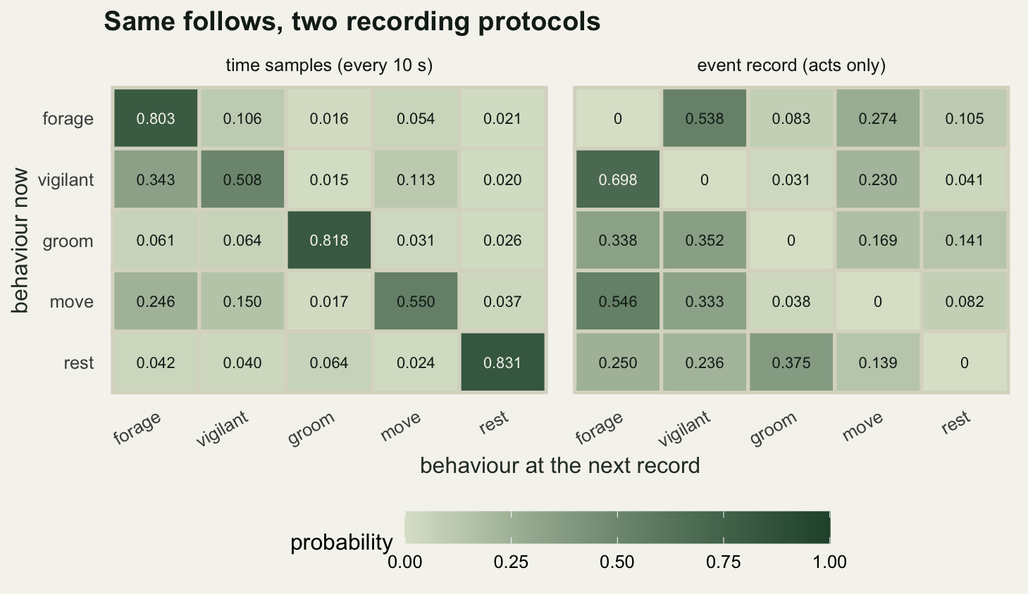
The picture makes the structural point faster than the numbers do. In the left panel the mass sits on the diagonal, because at a ten second glance an animal is usually doing what it was doing. In the right panel the diagonal is gone by construction and the mass has moved into the forage and vigilant columns: given that the animal has stopped whatever it was doing, foraging is the usual next act. Neither panel is wrong. They answer different questions, and “what does this animal do next” is ambiguous until you say whether “next” means the next ten seconds or the next act.
A practical note on which to collect. If you want bout durations, time budgets or anything that involves how long behaviours last, you need durations, so either time-sample or record onset times with your acts. If you only want the sequential structure of acts, the event record is fine and cheaper. What you cannot do is collect one and quote statistics that belong to the other.
Does the sequence actually have memory?
The Markov assumption is not free. Two questions are worth asking of any real record, and both are likelihood-ratio tests on a contingency table, which base R computes without any package at all.
The first order model says the next behaviour depends on the current one. The zero-order model says it does not: the record is a sequence of independent draws from a fixed distribution over behaviours. If a record fails to reject zero-order, the sequence carries no sequential information and you should stop and just report frequencies.
g2_independence <- function(N) {
  ri <- rowSums(N); ci <- colSums(N)
  expect <- outer(ri, ci) / sum(N)
  ok <- N > 0
  stat <- 2 * sum(N[ok] * log(N[ok] / expect[ok]))
  degf <- (sum(ri > 0) - 1) * (sum(ci > 0) - 1)
  c(G2 = stat, df = degf, p = pchisq(stat, degf, lower.tail = FALSE))
}

print(round(c(par_zero_order = n_state - 1,
              par_first_order = n_state * (n_state - 1),
              par_second_order = n_state^2 * (n_state - 1),
              df_zero_vs_first = (n_state - 1)^2), 0))
par_zero_order par_first_order par_second_order df_zero_vs_first
4 20 100 16 test_01 <- g2_independence(N_time)
print(round(test_01, 4)) G2 df p
4042.53 16.00 0.00 The zero-order model has 4 free parameters, the first-order model has 20, and the difference, 16, is the degrees of freedom. The statistic on the time-sampled record is 4042.53 on 16 degrees of freedom, and the p-value prints as 0 because it is smaller than the smallest number a double can hold. The record has sequential structure, which it had better, since it was generated with some.
Getting the degrees of freedom right matters more than it looks. The count is not “number of cells minus one”. It is the number of free parameters the larger model adds, and for a transition matrix each row is a probability vector, so each row contributes 4 free parameters and not 5. The function above also counts only rows and columns that were actually observed, which is what saves it when a behaviour never occurs in a short record.
The second question is harder. A second-order chain lets the next behaviour depend on the previous two. The null is the first-order chain, the alternative is a separate probability row for every ordered pair of preceding behaviours, and the count table is a five by five by five array.
count_triples <- function(x, S) {
  n <- length(x)
  i <- x[1:(n - 2)]; j <- x[2:(n - 1)]; k <- x[3:n]
  array(tabulate(((k - 1L) * S + (j - 1L)) * S + i, nbins = S^3), c(S, S, S))
}

g2_second <- function(N3) {
  S <- dim(N3)[1]
  n_ij <- apply(N3, c(1, 2), sum)
  n_jk <- apply(N3, c(2, 3), sum)
  n_j <- rowSums(n_jk)
  stat <- 0
  for (j in 1:S) if (n_j[j] > 0) {
    pr <- n_jk[j, ] / n_j[j]
    for (i in 1:S) if (n_ij[i, j] > 0) {
      obs <- N3[i, j, ]
      expect <- n_ij[i, j] * pr
      ok <- obs > 0
      stat <- stat + 2 * sum(obs[ok] * log(obs[ok] / expect[ok]))
    }
  }
  reach <- rowSums(n_jk > 0)
  seen <- colSums(n_ij > 0)
  degf <- sum(pmax(seen - 1, 0) * pmax(reach - 1, 0))
  c(G2 = stat, df = degf, p = pchisq(stat, max(degf, 1), lower.tail = FALSE))
}

N3_time <- array(0, c(n_state, n_state, n_state))
for (a in seq_len(n_animal)) N3_time <- N3_time + count_triples(paths[[a]], n_state)
test_12 <- g2_second(N3_time)
print(round(test_12, 4))
G2 df p
82.3531 80.0000 0.4064 print(round(c(nominal_df = n_state * (n_state - 1)^2,
cells_in_table = n_state^3,
triples_observed = sum(N3_time),
mean_count_per_cell = sum(N3_time) / n_state^3), 1)) nominal_df cells_in_table triples_observed mean_count_per_cell
80.0 125.0 3588.0 28.7 The statistic is 82.3531 on 80 degrees of freedom with a p-value of 0.4064. No evidence of second-order structure, correctly, because there is none in the generator.
The degrees of freedom deserve a second look, because this is where a five-state ethogram starts to hurt. The second-order model has 100 free parameters against the first-order model’s 20, a difference of 80. The count table has 125 cells and the record here supplies 3588 triples, so the average cell holds about 28.7 observations. The g2_second function counts degrees of freedom from the contexts and destinations that were actually observed rather than assuming all of them were, which is the standard adjustment for structural and sampling zeros; here everything was observed, so the adjusted count 80 equals the nominal 80.
How long a record does a second-order test need?
The honest question is not whether the test exists but whether your follow can support it. To measure that I need a process with real second-order structure, and there is a natural behavioural one: resumption. An animal that is interrupted tends to go back to what it was doing before the interruption. That makes the next behaviour depend on the behaviour two steps back, which is exactly second-order.
make_second_order <- function(P, delta) {
  S <- nrow(P)
  A <- array(0, c(S, S, S))
  for (i in 1:S) for (j in 1:S) {
    w <- P[j, ]
    if (i != j) w[i] <- w[i] * (1 + delta)
    A[i, j, ] <- w / sum(w)
  }
  dimnames(A) <- list(beh, beh, beh)
  A
}

sim_chain2 <- function(A, n, start = c(1L, 1L)) {
  S <- dim(A)[1]
  CP <- A
  for (i in 1:S) for (j in 1:S) CP[i, j, ] <- cumsum(A[i, j, ])
  u <- runif(n)
  x <- integer(n)
  x[1:2] <- start
  for (tt in 3:n) x[tt] <- 1L + sum(CP[x[tt - 2L], x[tt - 1L], ] < u[tt])
  x
}

delta_true <- 2
A_true <- make_second_order(P_true, delta_true)
print(round(c(resumption_multiplier = 1 + delta_true), 2))
resumption_multiplier
3 print(round(rbind(`first order, from vigilant` = P_true["vigilant", ],
`after move then vigilant` = A_true[4, 2, ],
`after groom then vigilant` = A_true[3, 2, ]), 3)) forage vigilant groom move rest
first order, from vigilant 0.300 0.550 0.020 0.110 0.020
after move then vigilant 0.246 0.451 0.016 0.270 0.016
after groom then vigilant 0.288 0.529 0.058 0.106 0.019The generator multiplies the probability of returning to the behaviour from two steps back by 3, then renormalises the row. An animal that was moving and is now vigilant has probability 0.270 of moving next, against 0.110 under the first-order chain, and one that was grooming and is now vigilant has probability 0.058 of grooming next against 0.020. Those are not subtle effects: the grooming one is a multiplier of three on the raw probability. If a test cannot find effects of that size, it cannot find anything.
The sweep below simulates records of five different lengths, runs the second-order test on each, and records how often it rejects at the five per cent level. It does the same on records generated by the plain first-order chain, so that the rejection rate under the null is measured rather than assumed. Two hundred replicates per length, which is enough to see the shape and keeps the whole post under a minute.
lens <- c(150, 300, 600, 1200, 2400)
n_rep <- 200
set.seed(20260728)
sweep_res <- data.frame(n = lens, power = 0, size = 0, mean_null_G2 = 0)
for (li in seq_along(lens)) {
  nn <- lens[li]
  hits <- 0
  false_hits <- 0
  null_stats <- numeric(n_rep)
  for (r in 1:n_rep) {
    g_alt <- g2_second(count_triples(sim_chain2(A_true, nn), n_state))
    if (g_alt[["p"]] < 0.05) hits <- hits + 1
    g_nul <- g2_second(count_triples(sim_chain(P_true, nn), n_state))
    null_stats[r] <- g_nul[["G2"]]
    if (g_nul[["p"]] < 0.05) false_hits <- false_hits + 1
  }
  sweep_res[li, ] <- c(nn, hits / n_rep, false_hits / n_rep,
                       round(mean(null_stats), 2))
}
print(round(c(replicates_per_length = n_rep, reference_df = n_state * (n_state - 1)^2), 0))
replicates_per_length reference_df
200 80 print(sweep_res) n power size mean_null_G2
1 150 0.100 0.005 31.20
2 300 0.125 0.000 43.48
3 600 0.295 0.000 58.72
4 1200 0.880 0.005 69.59
5 2400 1.000 0.040 81.05power_at <- approxfun(log(sweep_res$n), sweep_res$power)
grid_n <- exp(seq(log(min(lens)), log(max(lens)), length.out = 2000))
n_needed <- grid_n[which(power_at(log(grid_n)) >= 0.8)[1]]
print(round(c(n_for_power_0.8 = n_needed,
minutes_at_10s = n_needed * 10 / 60), 1))n_for_power_0.8 minutes_at_10s
1091.6 181.9 Power climbs from 0.100 at 150 records to 0.295 at 600 and 0.880 at 1200. Interpolating on the log scale, the test reaches eighty per cent power at about 1091.6 records, which at a ten second sampling interval is 181.9 minutes of continuous observation on a single animal. That is a long follow for one animal, and the effect being detected is a threefold change in a transition probability. Anything subtler needs more.
Here is the part I did not expect, and it changes how the power curve should be read. The rejection rate under the first-order null is 0.005 at 150 records, 0.000 at 300, and 0.000 at 600. Not five per cent. Essentially nothing. A test with a nominal size of 0.05 is refusing to reject at all, and only by 2400 records does it climb to 0.040, which is within Monte Carlo error of nominal for 200 replicates.
The mean statistic column says why. A chi-square variable on 80 degrees of freedom has a mean of 80, but the mean of the observed null statistic is 31.20 at 150 records and 58.72 at 600, reaching 81.05 only at 2400. With a 5-state ethogram the triple table has 125 cells, and at 150 records the counts are so thin that the likelihood-ratio statistic never gets near its asymptotic distribution. So the problem on a short follow is not only that power is low. The reference distribution is wrong, in the direction that makes the test refuse to speak, and both its size and its power are held down by the same fault.
That matters for how you report a negative result. “We tested for second-order dependence and found none” is a claim about the animal. On a 300 record follow it is a claim about the chi-square approximation, and the two are not the same sentence. If you need the test on a short record, calibrate it by simulation, exactly as the size column above does, rather than trusting the tabulated critical value.
curves <- rbind(
  data.frame(n = sweep_res$n, rate = sweep_res$power,
             series = "power (truth is second-order)"),
  data.frame(n = sweep_res$n, rate = sweep_res$size,
             series = "size (truth is first-order)"))

ggplot(curves, aes(n, rate, colour = series, shape = series)) +
  geom_hline(yintercept = 0.05, linetype = "dashed", colour = te_pal$clay) +
  geom_hline(yintercept = 0.8, linetype = "dotted", colour = te_pal$sage) +
  geom_line(linewidth = 0.9) +
  geom_point(size = 2.6) +
  annotate("text", x = 175, y = 0.845, label = "80% power",
           colour = te_pal$forest, size = 3.1, hjust = 0) +
  annotate("text", x = 1250, y = 0.135, label = "nominal 5%",
           colour = te_pal$clay, size = 3.1, hjust = 0) +
  scale_x_log10(breaks = lens, labels = lens) +
  scale_y_continuous(limits = c(0, 1)) +
  scale_colour_manual(values = c(te_pal$forest, te_pal$clay), name = NULL) +
  scale_shape_manual(values = c(16, 17), name = NULL) +
  labs(x = "records in the sequence (log scale)", y = "rejection rate",
       title = "The second-order test needs a very long follow") +
  theme_te()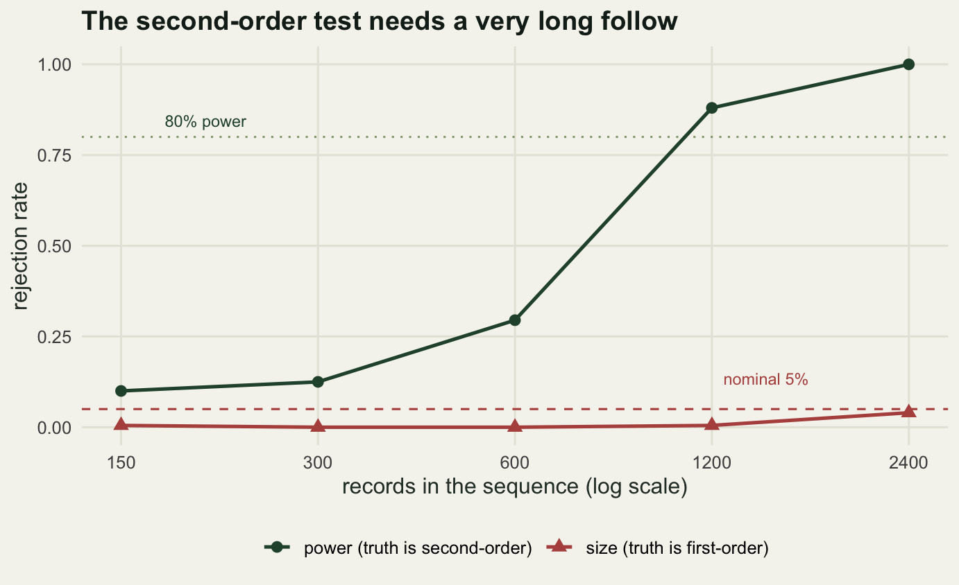
The stationary distribution, and why it is not the act distribution
A well behaved transition matrix has a distribution over behaviours that it leaves unchanged: a row vector pi with pi %*% P = pi. Run the chain long enough from anywhere and the fraction of samples in each state converges to pi. That is the long-run time budget, and it falls out of the leading left eigenvector.
stationary <- function(M) {
  ev <- eigen(t(M))
  v <- Re(ev$vectors[, which.max(Re(ev$values))])
  v / sum(v)
}

pi_time <- stationary(P_true); names(pi_time) <- beh
nu_act <- stationary(Q_from_P); names(nu_act) <- beh
occupancy <- tabulate(unlist(paths), n_state) / length(unlist(paths))
act_freq <- tabulate(unlist(acts), n_state) / length(unlist(acts))
names(occupancy) <- beh; names(act_freq) <- beh

print(round(rbind(stationary_of_P = pi_time, simulated_occupancy = occupancy,
                  stationary_of_jump_chain = nu_act,
                  simulated_act_frequency = act_freq), 4))
forage vigilant groom move rest
stationary_of_P 0.4669 0.1705 0.1034 0.1222 0.1370
simulated_occupancy 0.4942 0.1647 0.1089 0.1136 0.1186
stationary_of_jump_chain 0.3506 0.2880 0.0776 0.2066 0.0772
simulated_act_frequency 0.3604 0.2998 0.0739 0.1899 0.0760print(round(c(max_abs_time_error = max(abs(pi_time - occupancy)),
max_abs_act_error = max(abs(nu_act - act_freq))), 4))max_abs_time_error max_abs_act_error
0.0272 0.0166 The stationary distribution of P_true and the occupancy actually simulated agree to 0.0272 in the worst behaviour, over 3600 samples. The eigenvector is doing exactly what it claims. The same check on the jump chain agrees to 0.0166.
Now the part that is easy to get wrong, and I have seen it in print. The stationary distribution of the act chain is not a time budget. It is the long-run frequency of acts, and an act that lasts sixty seconds counts exactly as much as one that lasts ten.
converted <- nu_act * bout_true
converted <- converted / sum(converted)
print(round(rbind(time_budget = pi_time, act_share = nu_act,
                  act_share_times_bout = converted), 4))
forage vigilant groom move rest
time_budget 0.4669 0.1705 0.1034 0.1222 0.1370
act_share 0.3506 0.2880 0.0776 0.2066 0.0772
act_share_times_bout 0.4669 0.1705 0.1034 0.1222 0.1370print(round(c(rest_time_pct = 100 * pi_time[["rest"]],
rest_act_pct = 100 * nu_act[["rest"]],
vigilant_time_pct = 100 * pi_time[["vigilant"]],
vigilant_act_pct = 100 * nu_act[["vigilant"]],
largest_gap_pct = 100 * max(abs(nu_act - pi_time))), 2)) rest_time_pct rest_act_pct vigilant_time_pct vigilant_act_pct
13.70 7.72 17.05 28.80
largest_gap_pct
11.76 print(round(c(max_error_after_conversion = max(abs(converted - pi_time))), 6))max_error_after_conversion
0 Read the two rows against each other. Rest takes 13.70 per cent of the animal’s time but only 7.72 per cent of its acts, because rest bouts are long and each one is a single act. Vigilance is the mirror image: 17.05 per cent of time, 28.80 per cent of acts, because vigilance arrives in many short bouts. The largest disagreement between the two distributions is 11.76 percentage points. If you collected an event record, computed its stationary distribution and called it a time budget, that is the size of the error you would publish.
The fix is one multiplication. Weight each act by the mean duration of that behaviour’s bouts and renormalise, and the act distribution turns back into the time budget: after conversion the largest remaining error against the true stationary distribution is 0 to six decimal places, which is machine noise. This is why an event record without durations is not enough for a time budget, and why the standard advice to note the onset time of every act is not bureaucracy.
budget <- rbind(
  data.frame(behaviour = beh, value = as.numeric(pi_time),
             series = "time budget: stationary of P"),
  data.frame(behaviour = beh, value = as.numeric(occupancy),
             series = "occupancy actually simulated"),
  data.frame(behaviour = beh, value = as.numeric(nu_act),
             series = "act share: stationary of jump chain"))
budget$behaviour <- factor(budget$behaviour, levels = rev(beh))
budget$series <- factor(budget$series,
                        levels = c("time budget: stationary of P",
                                   "occupancy actually simulated",
                                   "act share: stationary of jump chain"))

ggplot(budget, aes(value, behaviour, colour = series, shape = series)) +
  geom_point(size = 3.4, stroke = 0.9, fill = NA) +
  scale_colour_manual(values = c(te_pal$forest, te_pal$gold, te_pal$clay),
                      name = NULL) +
  scale_shape_manual(values = c(16, 0, 17), name = NULL) +
  scale_x_continuous(limits = c(0, 0.55)) +
  guides(colour = guide_legend(nrow = 3), shape = guide_legend(nrow = 3)) +
  labs(x = "proportion", y = NULL,
       title = "An act budget is not a time budget") +
  theme_te()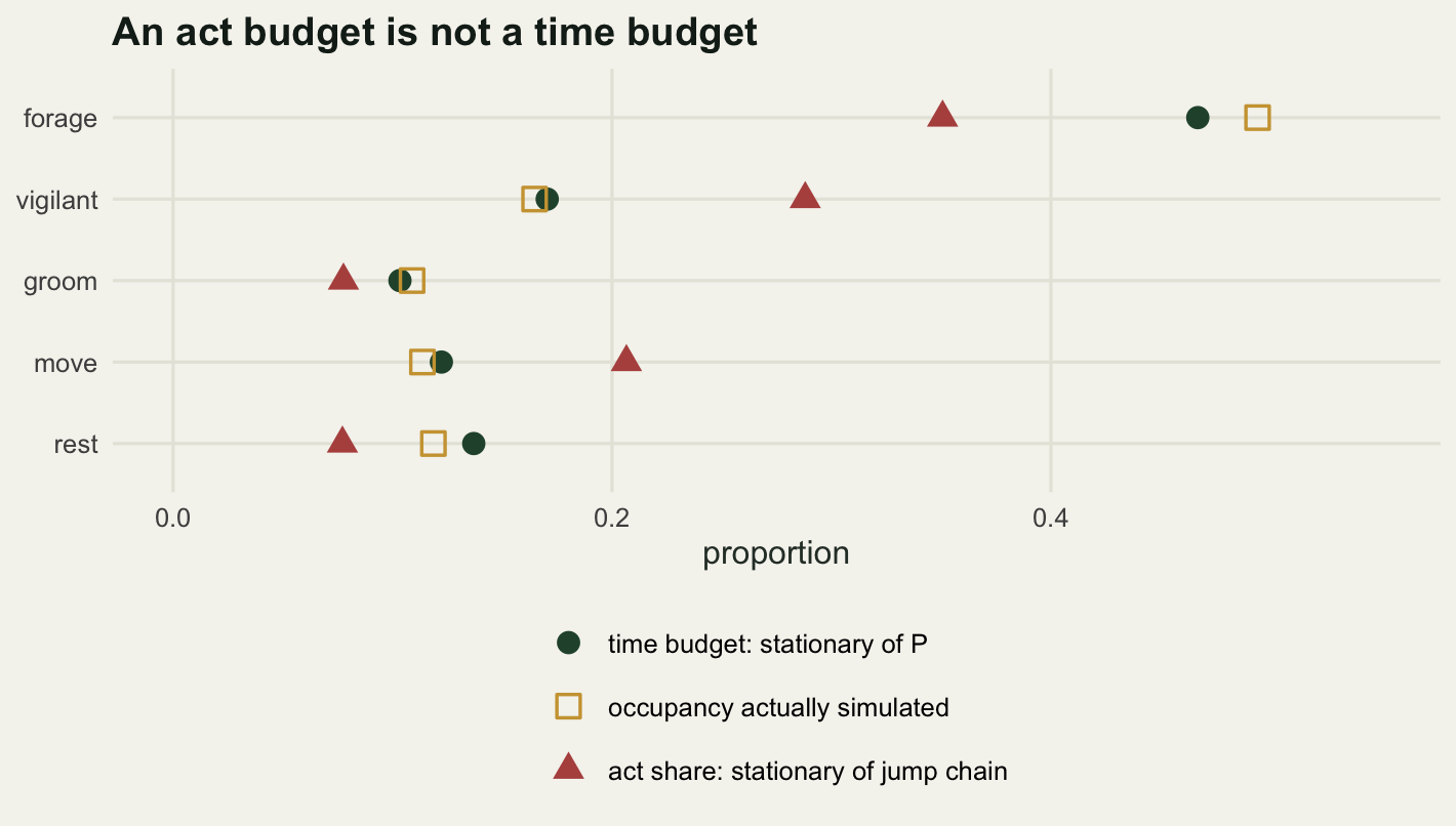
The figure is the argument in one look. The circles and the squares sit close together for every behaviour, never further apart than 0.0272, which is the eigenvector check passing: at forage and at rest the gap is wide enough to see, and it is the Monte Carlo scatter of 3600 simulated samples rather than a disagreement about the answer. The triangles are somewhere else entirely, and the direction of the error is systematic rather than random: long-bout behaviours are pushed down, short-bout behaviours are pushed up. A comparison between two populations that used act shares on one and time samples on the other would find a difference in vigilance that is entirely an artefact of the protocol.
Pooling animals, and a type I error that gets worse with more data
Everything so far pooled six animals into one count table. That was legitimate here for one reason only: the animals were generated from the same transition matrix, so a transition from animal one carries the same information as a transition from animal four. Real animals do not oblige. Individuals differ in how vigilant they are, and once they do, pooling their transitions into one contingency table treats between-animal variation as if it were within-animal signal.
The measurement below sets up the cleanest possible version of the mistake. Twelve animals, each with its own foraging row drawn around the population values, split at random into two groups of six. There is no group effect at all: group membership is a coin flip. The question is how often each of two tests declares a difference between the groups in the probability of going from foraging to vigilance.
rdirichlet1 <- function(alpha) {
  g <- rgamma(length(alpha), alpha, 1)
  g / sum(g)
}

kappa <- 60
set.seed(20260730)
spread <- sd(replicate(2000, rdirichlet1(kappa * P_true["forage", ])[2]))
print(round(c(concentration = kappa,
              population_p_forage_to_vigilant = P_true["forage", "vigilant"],
              between_animal_sd = spread), 4))
concentration population_p_forage_to_vigilant
60.000 0.100
between_animal_sd
0.039 The between-animal standard deviation in the probability of switching from foraging to vigilance is 0.039 around a population value of 0.1, so a typical animal sits somewhere between about six and fourteen per cent. That is a modest amount of individuality by the standards of any repeatability study I have read.
one_dataset <- function(n_per, n_an = 12) {
  n_vig <- integer(n_an); n_for <- integer(n_an); p_hat <- numeric(n_an)
  for (a in 1:n_an) {
    P_a <- P_true
    P_a[1, ] <- rdirichlet1(kappa * P_true["forage", ])
    N_a <- count_pairs(sim_chain(P_a, n_per), n_state)
    n_for[a] <- sum(N_a[1, ]); n_vig[a] <- N_a[1, 2]
    p_hat[a] <- n_vig[a] / n_for[a]
  }
  grp <- rep(1:2, each = n_an / 2)
  pooled <- rbind(c(sum(n_vig[grp == 1]), sum(n_for[grp == 1]) - sum(n_vig[grp == 1])),
                  c(sum(n_vig[grp == 2]), sum(n_for[grp == 2]) - sum(n_vig[grp == 2])))
  c(pooled = unname(g2_independence(pooled)[["p"]]),
    animal = t.test(p_hat[grp == 1], p_hat[grp == 2])$p.value)
}

n_rep2 <- 400
set.seed(20260729)
pvals <- list()
for (n_per in c(100, 400)) {
  pvals[[as.character(n_per)]] <- t(replicate(n_rep2, one_dataset(n_per)))
}
err <- data.frame(
  records_per_animal = c(100, 400),
  pooled = c(mean(pvals[["100"]][, 1] < 0.05), mean(pvals[["400"]][, 1] < 0.05)),
  animal_level = c(mean(pvals[["100"]][, 2] < 0.05),
                   mean(pvals[["400"]][, 2] < 0.05)))
print(round(c(datasets_per_setting = n_rep2, animals = 12, nominal_alpha = 0.05), 2))
datasets_per_setting animals nominal_alpha
400.00 12.00 0.05 print(err) records_per_animal pooled animal_level
1 100 0.1525 0.040
2 400 0.3125 0.035The pooled test rejects a null that is true 0.1525 of the time when each animal contributes 100 records, against a nominal 0.05. That is roughly a threefold inflation and it is the expected direction. The animal-level test, which reduces each animal to one number and then compares six numbers against six, rejects 0.040 of the time: near enough nominal for 400 datasets.
Now the number that surprised me. Lengthen every follow from 100 records to 400, which is four times the field effort, and the pooled test gets worse: 0.3125 instead of 0.1525, roughly double the error rate and more than six times nominal. The animal-level test is unmoved at 0.035.
That direction is worth sitting with, because the reflex is that more data cures statistical problems. Here it does the opposite, and the mechanism is not mysterious once you see it. Watching each animal for longer estimates each animal’s own transition probability more precisely, but it does nothing at all to the number of animals, which is where the between-animal variance lives. The pooled test computes its standard error from the total number of transitions, so more transitions mean a smaller standard error, while the quantity being compared still scatters by the full between-animal standard deviation of 0.039. Precision goes up, the thing it is measuring does not settle down, and the test rejects more often. Collecting longer follows to fix a pooled analysis makes the false positive rate go up, not down.
set.seed(20260801)
one_identical <- function(n_per, n_an = 12) {
  n_vig <- integer(n_an); n_for <- integer(n_an)
  for (a in 1:n_an) {
    N_a <- count_pairs(sim_chain(P_true, n_per), n_state)
    n_for[a] <- sum(N_a[1, ]); n_vig[a] <- N_a[1, 2]
  }
  grp <- rep(1:2, each = n_an / 2)
  pooled <- rbind(c(sum(n_vig[grp == 1]), sum(n_for[grp == 1]) - sum(n_vig[grp == 1])),
                  c(sum(n_vig[grp == 2]), sum(n_for[grp == 2]) - sum(n_vig[grp == 2])))
  unname(g2_independence(pooled)[["p"]])
}
p_identical <- replicate(n_rep2, one_identical(400))
print(round(c(pooled_type1_identical_animals = mean(p_identical < 0.05)), 4))
pooled_type1_identical_animals
0.0325 The control confirms where the fault lies. Repeat the whole thing with every animal sharing the same transition matrix, so that between-animal variation is zero, and the pooled test rejects 0.0325 of the time, which is fine. Pooling is not the sin. Pooling heterogeneous animals is, and since you cannot know in advance that your animals are homogeneous, the animal-level route is the default.
pv <- rbind(
  data.frame(p = pvals[["100"]][, 1], test = "pooled records", len = "100 records per animal"),
  data.frame(p = pvals[["100"]][, 2], test = "animal-level", len = "100 records per animal"),
  data.frame(p = pvals[["400"]][, 1], test = "pooled records", len = "400 records per animal"),
  data.frame(p = pvals[["400"]][, 2], test = "animal-level", len = "400 records per animal"))
pv$test <- factor(pv$test, levels = c("pooled records", "animal-level"))

ggplot(pv, aes(p)) +
  geom_histogram(breaks = seq(0, 1, by = 0.05), fill = te_pal$green,
                 colour = te_pal$paper, linewidth = 0.4) +
  geom_hline(yintercept = n_rep2 / 20, linetype = "dashed",
             colour = te_pal$clay, linewidth = 0.7) +
  facet_grid(len ~ test) +
  labs(x = "p-value under a true null", y = "datasets",
       title = "Pooled tests fail, and fail harder with longer follows") +
  theme_te() +
  theme(legend.position = "none")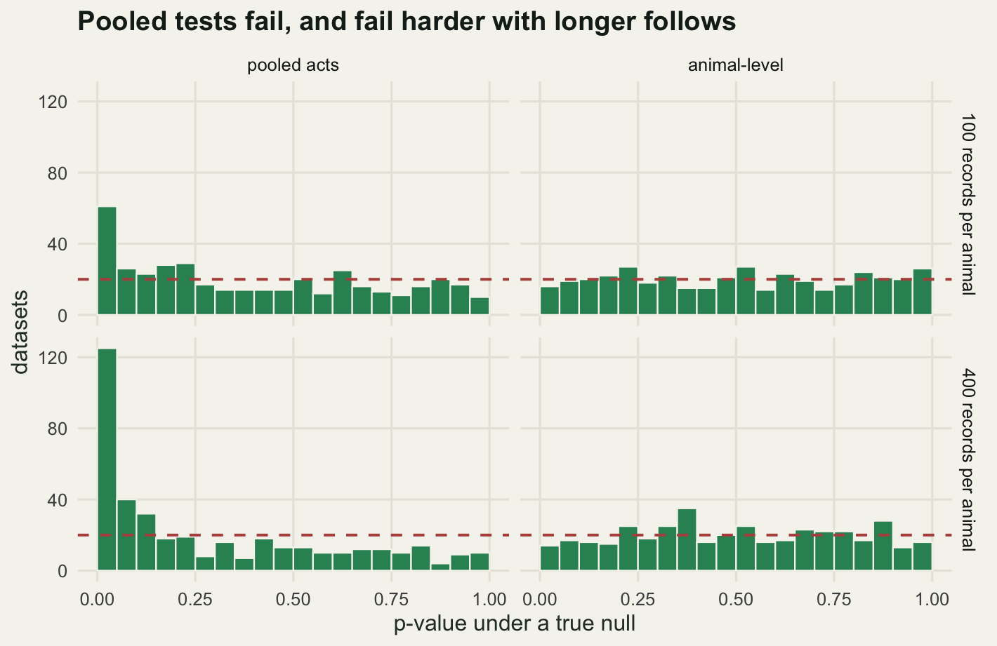
The right-hand column is what a working test looks like: p-values spread evenly across the interval, because under a true null a p-value is uniform by construction. The left-hand column is what a pooled test looks like, and the comparison between its two rows is the measurement that matters. More field effort per animal made the histogram spike higher.
If you take one operational rule from this post, take this one. Estimate the transition matrix per animal, then do the statistics on the animal-level quantities: the transition probability of interest, or a diversity index of the matrix, or whatever summary answers your question. Twelve animals give you twelve numbers. That feels like a painfully small dataset after a fortnight in the field, and it is the honest one. There is more on the general shape of this problem in pseudoreplication and false positives in ecology and, for the variance-partitioning version, in checking a repeatability analysis.
What to take away
The mechanics are genuinely easy. A transition matrix is a table of counts divided by its row sums, the memory tests are likelihood-ratio statistics on that table with degrees of freedom you can count on your fingers, and the time budget is an eigenvector. None of it needs a package. What is not easy is knowing which of two matrices you have estimated, and the measurements above put numbers on the cost of getting that wrong: up to 0.831 in probability units between the time-sampled and event-record matrices for the same animals, and 11.76 percentage points between an act share and a time budget.
Two results went against what I expected when I started. The second-order test does not fail gracefully on a short record: at 150 and 300 records its rejection rate under a true null is 0.005 and 0.000 against a nominal 0.05, so a negative result there says nothing about the animal. And the pooled test across heterogeneous animals gets worse with more data, moving from 0.1525 to 0.3125 when follows lengthen from 100 to 400 records, which inverts the usual instinct that a bigger sample is a safer one.
Now the honest limit, and it is a limit on the whole approach rather than on any one test. The Markov assumption is a modelling choice that a test can reject but never confirm. Failing to reject first-order structure means your record was not long enough, or your states were not fine enough, to see the memory: it does not mean the memory is absent. The second point is sharper. A coarse ethogram can make a genuinely non-Markov process look Markov, by hiding inside one label the state that carries the memory. Lump “forage” and “handle prey” into a single foraging category and the dependence on how long the animal has already been foraging disappears into the category, and the chain that comes out will pass every test you throw at it. The transition matrix is a description of the ethogram you chose at least as much as it is a description of the animal, so write down the ethogram definitions with the results and treat a passed Markov test as a statement about your categories rather than about behaviour itself.
References
Altmann J 1974 Behaviour 49(3-4):227-267 (10.1163/156853974X00534)
Hurlbert SH 1984 Ecological Monographs 54(2):187-211 (10.2307/1942661)
Patterson TA, Basson M, Bravington MV, Gunn JS 2009 Journal of Animal Ecology 78(6):1113-1123 (10.1111/j.1365-2656.2009.01583.x)
Langrock R, King R, Matthiopoulos J, Thomas L, Fortin D, Morales JM 2012 Ecology 93(11):2336-2342 (10.1890/11-2241.1)
Bakeman R, Gottman JM 1997 Observing Interaction: An Introduction to Sequential Analysis, second edition (ISBN 978-0-521-57427-3)
Zucchini W, MacDonald IL, Langrock R 2016 Hidden Markov Models for Time Series: An Introduction Using R, second edition (ISBN 978-1-4822-5383-2)