library(ggplot2)
library(dplyr)
library(tidyr)

pal <- list(ink = "#16241d", body = "#2c3a31", forest = "#275139", label = "#46604a",
            sage = "#93a87f", paper = "#f5f4ee", line = "#dad9ca", faint = "#5d6b61")
st3 <- c("#cda23f", "#b5534e", "#275139")
theme_te <- function(base_size = 12) {
  theme_minimal(base_size = base_size) +
    theme(plot.background = element_rect(fill = pal$paper, colour = NA),
          panel.background = element_rect(fill = pal$paper, colour = NA),
          panel.grid.major = element_line(colour = pal$line, linewidth = 0.3),
          panel.grid.minor = element_blank(),
          axis.text = element_text(colour = pal$faint), axis.title = element_text(colour = pal$body),
          plot.title = element_text(colour = pal$ink, face = "bold"),
          plot.subtitle = element_text(colour = pal$label),
          strip.text = element_text(colour = pal$ink, face = "bold"),
          legend.text = element_text(colour = pal$body), legend.position = "top")
}

dvm <- function(theta, mu, kappa) exp(kappa * cos(theta - mu)) / (2 * pi * besselI(kappa, 0))
rvm <- function(n, mu, kappa) {
  mu <- rep(mu, length.out = n); kappa <- rep(kappa, length.out = n); out <- numeric(n)
  for (i in 1:n) {
    k <- kappa[i]; a <- 1 + sqrt(1 + 4 * k^2); b <- (a - sqrt(2 * a)) / (2 * k); r <- (1 + b^2) / (2 * b)
    repeat {
      u1 <- runif(1); u2 <- runif(1); u3 <- runif(1)
      z <- cos(pi * u1); f <- (1 + r * z) / (r + z); cc <- k * (r - f)
      if (cc * (2 - cc) - u2 > 0 || log(cc / u2) + 1 - cc >= 0) { out[i] <- sign(u3 - 0.5) * acos(f) + mu[i]; break }
    }
  }
  ((out + pi) %% (2 * pi)) - pi
}
mkGamma <- function(eta, N) {
  G <- diag(N); if (N == 1) return(G); idx <- 1
  for (i in 1:N) { e <- numeric(N)
    for (j in setdiff(1:N, i)) { e[j] <- eta[idx]; idx <- idx + 1 }
    num <- exp(e); G[i, ] <- num / sum(num) }
  G
}
w2n_gen <- function(w, N) {
  ntr <- N * (N - 1); eta <- if (ntr > 0) w[1:ntr] else numeric(0); rest <- w[(ntr + 1):length(w)]
  list(Gamma = mkGamma(eta, N), shape = exp(rest[1:N]),
       scale = exp(rest[(N + 1):(2 * N)]), kappa = exp(rest[(2 * N + 1):(3 * N)]))
}
statdist <- function(G) { N <- nrow(G); if (N == 1) return(1); solve(t(diag(N) - G + 1), rep(1, N)) }
allprobs_gen <- function(p, step, turn, N) {
  Tn <- length(step); ap <- matrix(1, Tn, N)
  for (j in 1:N) ap[, j] <- dgamma(step, shape = p$shape[j], scale = p$scale[j]) *
    ifelse(is.na(turn), 1, dvm(turn, 0, p$kappa[j]))
  ap
}
nll_gen <- function(w, step, turn, N) {
  p <- w2n_gen(w, N); Tn <- length(step); ap <- allprobs_gen(p, step, turn, N)
  if (any(!is.finite(ap))) return(1e10)
  if (N == 1) return(-sum(log(pmax(ap[, 1], 1e-300))))
  delta <- tryCatch(statdist(p$Gamma), error = function(e) rep(1 / N, N))
  foo <- delta * ap[1, ]; s <- sum(foo); if (s <= 0) return(1e10); ls <- log(s); foo <- foo / s
  for (t in 2:Tn) { foo <- (foo %*% p$Gamma) * ap[t, ]; s <- sum(foo); if (s <= 0) return(1e10); ls <- ls + log(s); foo <- foo / s }
  -ls
}
npar_hmm <- function(N) N * (N - 1) + 3 * N
emis_start <- function(step, N) {
  qs <- quantile(step, probs = seq(0, 1, length.out = N + 1)); sh <- sc <- ka <- numeric(N)
  for (j in 1:N) { grp <- step[step >= qs[j] & step <= qs[j + 1]]
    m <- mean(grp); v <- var(grp); sh[j] <- max(m^2 / v, 0.3); sc[j] <- v / m; ka[j] <- 1 }
  c(log(sh), log(sc), log(ka))
}How many states in a movement HMM?
ecology tutorial
movement ecology
hidden Markov models
Choose how many states a movement HMM needs without overfitting: AIC and BIC across candidate models, why an extra state splits a real one, and label switching.
Corrected 27 September 2026: the fitting code polished only the best Nelder-Mead endpoint, so the three- and four-state fits in the table were not the best found, and the optima were counted on unpolished endpoints. Every endpoint is now polished: the three-state model sits 1.77 above the best AIC rather than 5.51, the 18 starts reach 7 distinct optima rather than 16, and two states is still the choice of both criteria.
A two-state movement HMM assumes there are two behaviours. Real animals may have more, and the number is never given to us. It is tempting to add states until the fit stops improving, but the likelihood never stops improving: more states always fit the data at least as well. The question is not which model has the highest likelihood, but which has enough states to capture the behaviour and no more. This post fits movement HMMs with one to four states to the same track, uses AIC and BIC to choose, and then looks at two failure modes that a single fitted model hides: an extra state that merely splits a real one, and label switching across restarts.
We reuse the two-state track from the foundation post, simulated from a known two-state process, so we know the honest answer is two and can watch each criterion find it or miss it.
Setup and the general engine
The engine is a general \(N\)-state HMM: gamma step lengths, von Mises turning angles, and a transition matrix built from a multinomial logit whose reference category is staying in the current state. An \(N\)-state model has \(N(N-1)\) transition parameters and \(3N\) emission parameters.
The same track, re-simulated
Gamma_true <- matrix(c(0.90, 0.10, 0.15, 0.85), 2, 2, byrow = TRUE)
shape_true <- c(2, 4); scale_true <- c(20, 50); kappa_true <- c(0.7, 3.0); Tn <- 500
delta_true <- solve(t(diag(2) - Gamma_true + 1), rep(1, 2))
set.seed(4517)
S <- integer(Tn); S[1] <- sample(1:2, 1, prob = delta_true)
for (t in 2:Tn) S[t] <- sample(1:2, 1, prob = Gamma_true[S[t - 1], ])
step <- rgamma(Tn, shape = shape_true[S], scale = scale_true[S])
phi <- rvm(Tn, 0, kappa_true[S]); turn <- phi; turn[1] <- NA   # same RNG stream as the foundation post
Fitting one to four states
For each \(N\) we run many Nelder-Mead searches from jittered starts and polish every endpoint with a short BFGS pass. This matters here: with three or more states the likelihood surface has many local optima, and a single start is not enough. We keep the best fit for the table and, for the three-state model, keep every endpoint so we can see the spread.
multistart <- function(N, nstart, seed, nm_maxit = 1500) {
  set.seed(seed); vals <- numeric(0); bestf <- NULL
  for (s in 1:nstart) {
    jit <- if (s == 1) 0 else 0.7
    w0 <- c(if (N > 1) rep(-1.5, N * (N - 1)) + rnorm(N * (N - 1), 0, jit) else numeric(0),
            emis_start(step, N) + rnorm(3 * N, 0, jit))
    f <- try(optim(w0, nll_gen, step = step, turn = turn, N = N, method = "Nelder-Mead",
                   control = list(maxit = nm_maxit, reltol = 1e-11)), silent = TRUE)
    if (inherits(f, "try-error")) next
    fp <- try(optim(f$par, nll_gen, step = step, turn = turn, N = N, method = "BFGS",
                    control = list(maxit = 200, reltol = 1e-12)), silent = TRUE)
    if (!inherits(fp, "try-error") && fp$value < f$value) f <- fp
    vals <- c(vals, f$value)
    if (is.null(bestf) || f$value < bestf$value) bestf <- f
  }
  list(vals = vals, fit = bestf)
}
plan <- list(c(N = 1, ns = 3, sd = 511), c(N = 2, ns = 5, sd = 512),
             c(N = 3, ns = 18, sd = 513), c(N = 4, ns = 10, sd = 514))
tab <- data.frame(); fits <- list(); ls3 <- NULL
for (pl in plan) {
  m <- multistart(pl["N"], pl["ns"], pl["sd"]); f <- m$fit; N <- pl["N"]; k <- npar_hmm(N)
  fits[[N]] <- f; if (N == 3) ls3 <- m$vals
  tab <- rbind(tab, data.frame(states = N, npar = k, logLik = round(-f$value, 2),
                               AIC = round(2 * f$value + 2 * k, 2),
                               BIC = round(2 * f$value + k * log(Tn), 2), conv = f$convergence))
}
tab$dAIC <- round(tab$AIC - min(tab$AIC), 2); tab$dBIC <- round(tab$BIC - min(tab$BIC), 2)knitr::kable(tab, align = "r", row.names = FALSE, caption = "Movement HMMs with one to four states.")| states | npar | logLik | AIC | BIC | conv | dAIC | dBIC |
|---|---|---|---|---|---|---|---|
| 1 | 3 | -3642.00 | 7290.01 | 7302.65 | 0 | 317.35 | 296.28 |
| 2 | 8 | -3478.33 | 6972.66 | 7006.37 | 0 | 0.00 | 0.00 |
| 3 | 15 | -3472.22 | 6974.43 | 7037.65 | 0 | 1.77 | 31.28 |
| 4 | 24 | -3465.72 | 6979.44 | 7080.59 | 0 | 6.78 | 74.22 |
The log-likelihood climbs at every step, from -3642 at one state to -3465.72 at four, so on likelihood alone more is always better. The jump from one to two states is large, 163.7 in log-likelihood; every jump after that is small. AIC and BIC both add a penalty for parameters. AIC is minimised at 2 states, BIC at 2. The three-state model sits 1.77 above the best AIC and 31.28 above the best BIC; the four-state model 6.78 and 74.22. BIC penalises more heavily: its penalty per parameter is the log of the track length, while AIC’s does not depend on the track at all, so the two criteria pull apart further with every state added.
lng <- tab %>% select(states, AIC, BIC) %>% pivot_longer(-states, names_to = "criterion", values_to = "value")
best <- data.frame(criterion = c("AIC", "BIC"),
                   states = c(tab$states[which.min(tab$AIC)], tab$states[which.min(tab$BIC)]),
                   value = c(min(tab$AIC), min(tab$BIC)))
ggplot(lng, aes(states, value, colour = criterion)) +
  geom_line(linewidth = 0.8) + geom_point(size = 2.4) +
  geom_point(data = best, shape = 21, size = 4.5, stroke = 1.1, fill = NA) +
  scale_colour_manual(values = c(AIC = "#275139", BIC = "#b5534e"), name = NULL) +
  scale_x_continuous(breaks = 1:4) +
  labs(title = "Model selection across state numbers",
       subtitle = "Open circles mark the lowest point of each criterion",
       x = "Number of states", y = "Information criterion") + theme_te()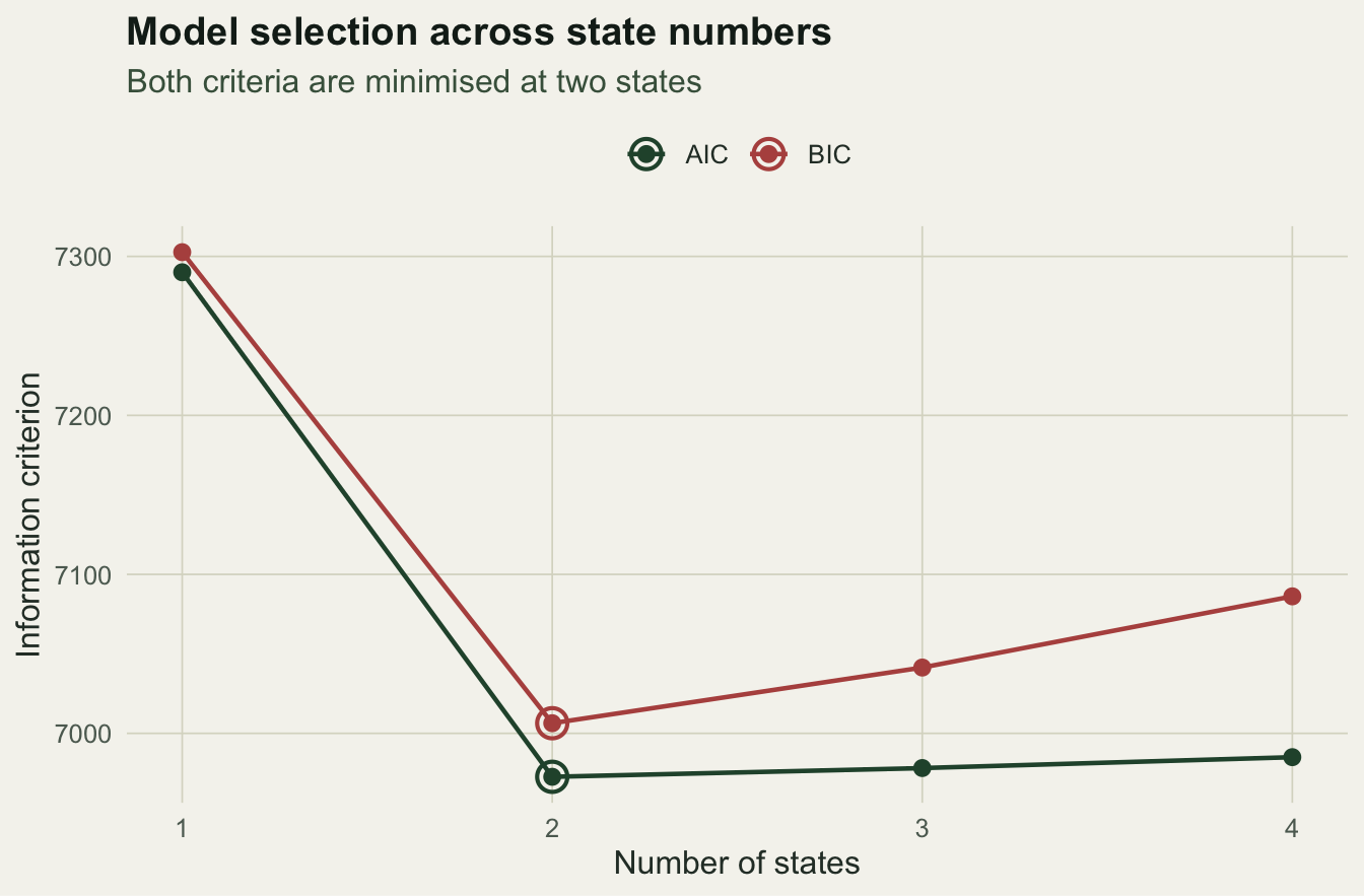
What the third state actually does
It helps to look at where the extra state goes rather than trusting the number alone. We compare the fitted step-length distributions of the two-state and three-state models. If the third state were a genuinely new behaviour it would sit apart from the other two. Instead it lands on top of an existing one.
p2 <- w2n_gen(fits[[2]]$par, 2); m2 <- p2$shape * p2$scale; o2 <- order(m2)
p3 <- w2n_gen(fits[[3]]$par, 3); m3 <- p3$shape * p3$scale; o3 <- order(m3)
The two-state means are 44.1 m and 203.6 m. The three-state means are 43.7, 182.6 and 209.4 m. One of the two modes survives almost unchanged, and the other has been cut in two. The third state is not a new movement mode; it is a finer description of behaviour the two-state model already had, bought with seven extra parameters.
gx <- seq(0, 620, length.out = 400)
dl2 <- statdist(p2$Gamma); dl3 <- statdist(p3$Gamma)
lab2 <- c("State 1", "State 2"); lab3 <- c("State 1", "State 2", "State 3")
c2 <- do.call(rbind, lapply(seq_along(o2), function(k) { j <- o2[k]
  data.frame(x = gx, dens = dl2[j] * dgamma(gx, p2$shape[j], scale = p2$scale[j]), state = lab2[k], model = "Two states") }))
c3 <- do.call(rbind, lapply(seq_along(o3), function(k) { j <- o3[k]
  data.frame(x = gx, dens = dl3[j] * dgamma(gx, p3$shape[j], scale = p3$scale[j]), state = lab3[k], model = "Three states") }))
cc <- rbind(c2, c3); cc$model <- factor(cc$model, levels = c("Two states", "Three states"))
hh <- rbind(data.frame(step = step, model = "Two states"), data.frame(step = step, model = "Three states"))
hh$model <- factor(hh$model, levels = c("Two states", "Three states"))
ggplot() +
  geom_histogram(data = hh, aes(step, after_stat(density)), bins = 45, fill = pal$sage, alpha = 0.3) +
  geom_line(data = cc, aes(x, dens, colour = state), linewidth = 0.9) +
  facet_wrap(~model) + scale_colour_manual(values = st3, name = NULL) +
  labs(title = "Fitted step-length densities, two states and three",
       subtitle = "The same histogram of steps under each model",
       x = "Step length (m)", y = "Density") + theme_te()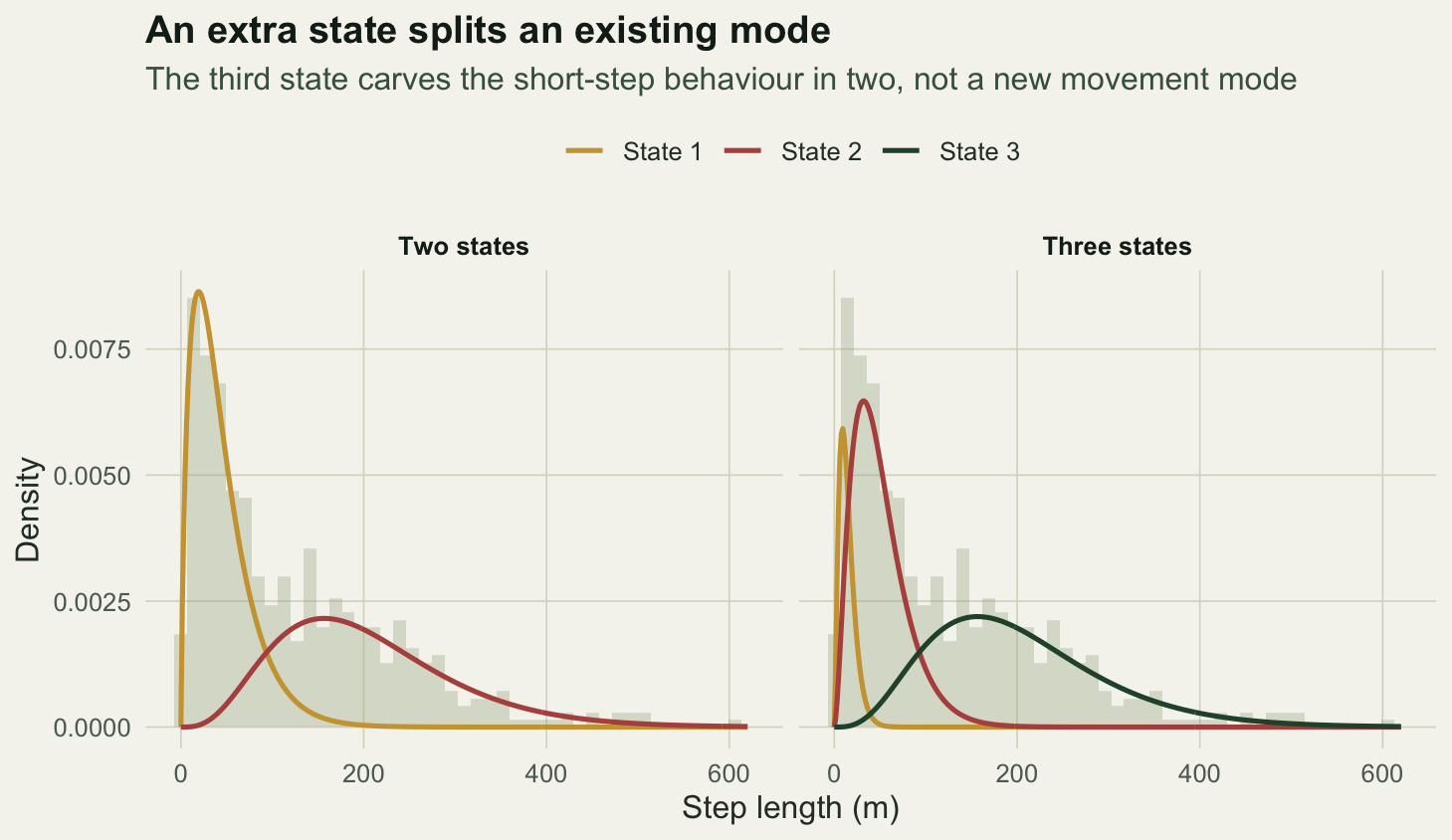
Label switching and local optima
The multi-start pass was not decoration. States in an HMM have no inherent order, so the labels can permute without changing the likelihood, and the surface for three states is riddled with local optima on top of that. Our 18 starts for the three-state model reached 7 distinct optima. The best negative log-likelihood found was 3472.2, the worst 3475.8, a spread of 3.5, and only 17% of starts landed within half a unit of the best. A single run from a single start would have reported one of these, quite possibly not the best, with no warning. Any HMM with more than two states should be fitted from many starts, and the fit reported is the best of them.
The rule of thumb, and its limits
Fit a range of state numbers, compare with AIC and BIC, and treat a disagreement between them as a signal to look harder rather than to average. But information criteria are a guide, not a verdict. They can favour an extra state that soaks up a quirk of one distribution rather than a real behaviour, which is why the inspection above matters: a state worth keeping should be interpretable, separated in the emissions, and occupied for a reasonable share of the track. Cross-validation on held-out tracks and pseudo-residual checks give a fuller picture than either criterion alone. The honest summary is that model selection narrows the field; biology decides.
References
Celeux G, Durand J-B 2008 Computational Statistics 23(4):541-564 (10.1007/s00180-007-0097-1)
Langrock R, King R, Matthiopoulos J, Thomas L, Fortin D, Morales JM 2012 Ecology 93(11):2336-2342 (10.1890/11-2241.1)
Pohle J, Langrock R, van Beest FM, Schmidt NM 2017 Journal of Agricultural, Biological and Environmental Statistics 22(3):270-293 (10.1007/s13253-017-0283-8)
Zucchini W, MacDonald IL, Langrock R 2016 Hidden Markov Models for Time Series: An Introduction Using R (2nd ed.). CRC Press. ISBN 978-1-4822-5383-2