Reversible jump MCMC from scratch

Code a reversible jump sampler by hand in R to count abundance zones on a saltmarsh transect, and check its model probabilities against exact enumeration.

A saltmarsh transect: sixty contiguous quadrats, each half a metre square, laid end to end along a thirty metre line that starts in the upper marsh and runs down across the transition into the mid marsh. In every quadrat somebody counted a small grazing snail. The counts are low, in single figures for most of the line, and they are visibly higher at the upper end than at the lower end.

The ecological question is not how steep the gradient is. Saltmarsh zonation is usually described as a set of bands with reasonably sharp edges, so the natural model is a step function: the snail sits at one density for a stretch of the transect, then changes abruptly at a boundary, then sits at another density. The quantity of interest is the number of boundaries, and it cannot be answered by fitting one model. A model with k boundaries has k positions and k + 1 densities, so moving from one boundary to two adds two numbers to the parameter vector. The models live on spaces of different dimension, and an ordinary sampler cannot walk between them. Reversible jump Markov chain Monte Carlo, introduced by Green (1995), is the construction that lets a single chain treat the model index as one more thing to be sampled.

This post sits in a cluster of Bayesian computation posts and does something none of them does. Metropolis-Hastings from scratch builds the sampler this one extends: the acceptance ratio below is that post’s likelihood-times-prior ratio with two extra factors bolted on, a proposal density for the new parameter and a Jacobian, and the derivation shows exactly where the two come from. Bayesian model comparison: WAIC, LOO, DIC scores a fixed list of candidates by how well each predicts held-out data, which is a different question from the posterior probability of each model, and the two can disagree: a model can predict best and still carry little posterior probability, because a predictive score does not charge for prior spread and a model probability does. How many states in a movement HMM? is the applied version of the same worry, and it already covers label switching and local optima, so none of that is repeated here.

The sharpest contrast is with the two marginal likelihood posts. The Laplace approximation in R computes a marginal likelihood by curvature at the mode, and the sibling post Bridge sampling for marginal likelihoods estimates one by an importance-style identity. Reversible jump gets the posterior probability of every model without computing a single marginal likelihood: the chain spends time in each model in proportion to its probability, and the answer is a set of visit frequencies. That is the appeal, and the price is a piece of bookkeeping that fails silently.

library(ggplot2)

te_pal <- list(forest = "#275139", green = "#2f8f63", sage = "#93a87f",
               clay = "#b5534e", gold = "#cda23f", line = "#dad9ca",
               ink = "#16241d", paper = "#f5f4ee")

theme_te <- function() {
  theme_minimal(base_size = 12) +
    theme(panel.grid.minor = element_blank(),
          panel.grid.major = element_line(colour = "#e7e6dc"),
          plot.background = element_rect(fill = "#f5f4ee", colour = NA),
          panel.background = element_rect(fill = "#f5f4ee", colour = NA),
          plot.title = element_text(face = "bold", colour = te_pal$ink),
          axis.title = element_text(colour = "#2c3a31"),
          axis.text = element_text(colour = "#2c3a31"))
}

The transect

The counts are synthetic, generated from a step function with one boundary, so every error below is a distance from a value that was set rather than an argument about what should have happened. The contrast across the boundary is deliberately modest: a large step would make the model comparison trivial and hide everything this post is about.

n_q <- 60
quad_side <- 0.5
quad_area <- quad_side^2
tau_true <- 24L
dens_true <- c(6.5, 5)

set.seed(20260803)
zone_true <- ifelse(seq_len(n_q) <= tau_true, 1L, 2L)
y <- rpois(n_q, dens_true[zone_true])

csum <- c(0, cumsum(y))
cfac <- c(0, cumsum(lgamma(y + 1)))

print(y)

 [1]  3  6  4 11  8  6  5  7  7  4  7  3  5 12 13  7  7  5  6  6  9  5  7  5  4
[26]  6  6  1  3  3  6  4  9  2  8  5  7  4  3  5  4  5  2  3  5  5  8  4  3  2
[51]  3  3  8  3  4  4  4  4  3  6

print(round(c(quadrats = n_q, quadrat_area_m2 = quad_area,
              total_snails = sum(y), mean_per_quadrat = mean(y),
              mean_upper = mean(y[seq_len(tau_true)]),
              mean_lower = mean(y[(tau_true + 1):n_q]),
              true_boundary = tau_true), 4))

        quadrats  quadrat_area_m2     total_snails mean_per_quadrat 
         60.0000           0.2500         317.0000           5.2833 
      mean_upper       mean_lower    true_boundary 
          6.5833           4.4167          24.0000 

The transect holds 317 snails in 60 quadrats, an average of 5.283 per quadrat. The first 24 quadrats average 6.583 and the remaining 36 average 4.417. A drop of that size in counts of this size is not obvious by eye, which is the point: the number of boundaries is genuinely uncertain here, and a method that only ever returns a confident answer is not being tested.

The model set runs from zero to three boundaries. Write \(M_k\) for the model with \(k\) boundaries at positions \(\tau_1 < \dots < \tau_k\) taken from the \(n - 1\) gaps between quadrats, and \(\lambda_1, \dots, \lambda_{k+1}\) for the expected count per quadrat in each zone. Counts are Poisson with the rate of their zone. The prior puts equal weight on the four values of \(k\), spreads the positions uniformly over the \(\binom{n-1}{k}\) ways of choosing them, and gives each zone rate an independent Gamma prior with shape one, which is an exponential distribution.

a_pr <- 1; b_pr <- 0.1; k_max <- 3
print(round(c(prior_shape = a_pr, prior_rate = b_pr, prior_mean_rate = a_pr / b_pr,
              prior_sd_rate = sqrt(a_pr) / b_pr, max_boundaries = k_max), 4))

    prior_shape      prior_rate prior_mean_rate   prior_sd_rate  max_boundaries 
            1.0             0.1            10.0            10.0             3.0 

The prior on a zone rate has mean 10 snails per quadrat and standard deviation 10, which is vague relative to an observed mean of 5.283 without being absurd. That choice matters more than it looks, and the last section measures how much.

What a fixed-dimension sampler cannot do

The Metropolis rule accepts a proposal with probability equal to the ratio of the target density at the proposed point and at the current point, capped at one. It comes out of detailed balance, and that derivation requires both densities to be densities of the same measure. Inside one model that is automatic. Across models it fails: the parameter vector of \(M_1\) has three entries and that of \(M_2\) has five, so the two posteriors live on spaces of three and five dimensions and their ratio is not a ratio of probabilities.

The failure is visible in the units. A density for the rates in \(M_k\) has units of (snails per quadrat) to the power \(-(k+1)\), because it integrates over \(k+1\) rates to give a pure number. Divide the density in \(M_2\) by the density in \(M_1\) and one power of snails per quadrat survives. A quantity with units cannot be a probability, and its value depends on whether abundance is recorded per quadrat or per square metre. Nothing in the code notices: the chain runs, it moves between models, and it converges to a distribution that changes when the field notebook changes its units. That claim is measured later, on the same data with the same seed.

Green’s fix is dimension matching. To move from a model with \(d\) parameters to one with \(d'\) parameters, where \(d' > d\), draw an auxiliary vector \(u\) of length \(d' - d\) from a density \(q(u)\), and give a smooth, invertible map \((\theta, u) \mapsto \theta'\). Both sides of the move now have the same number of coordinates, the change of variables theorem applies, and the acceptance probability is \(\min(1, A)\) with

\[A = \underbrace{\frac{p(y \mid \theta', M')}{p(y \mid \theta, M)}}_{\text{likelihood}} \times \underbrace{\frac{p(\theta' \mid M')\,p(M')}{p(\theta \mid M)\,p(M)}}_{\text{prior}} \times \underbrace{\frac{r(\theta')}{r(\theta)\,q(u)}}_{\text{proposal}} \times \underbrace{\left| \frac{\partial \theta'}{\partial (\theta, u)} \right|}_{\text{Jacobian}}\]

where \(r(\theta)\) is the probability of choosing this move from \(\theta\) and \(r(\theta')\) the probability of choosing the reverse move from \(\theta'\). The first two factors are what Metropolis-Hastings from scratch already computes. The third is the ordinary Hastings correction, extended to cover the auxiliary draw. The fourth has no counterpart in a fixed-dimension sampler, and it is the one that gets left out.

The exact answer, by enumeration

Before writing any sampler, work out what it should produce. With a Gamma prior on a Poisson rate the rate integrates out in closed form: for a zone covering quadrats \(i\) to \(j\), with \(S\) snails in \(m\) quadrats,

\[p(y_{i:j}) = \frac{b^a}{\Gamma(a)} \cdot \frac{\Gamma(a + S)}{(b + m)^{a + S}} \cdot \prod_{l=i}^{j} \frac{1}{y_l!}\]

so the marginal likelihood of a segmentation is a product of \(k+1\) such terms, and the marginal likelihood of the model is the average of that product over all \(\binom{n-1}{k}\) segmentations. The average can be accumulated by dynamic programming rather than enumerated one at a time.

log_sum_exp <- function(v) {
  mx <- max(v)
  if (!is.finite(mx)) return(-Inf)
  mx + log(sum(exp(v - mx)))
}

seg_lml <- function(i, j, rate = b_pr) {
  ss <- csum[j + 1] - csum[i]; mm <- j - i + 1
  a_pr * log(rate) - lgamma(a_pr) + lgamma(a_pr + ss) -
    (a_pr + ss) * log(rate + mm) - (cfac[j + 1] - cfac[i])
}

model_lml <- function(rate = b_pr, kmx = k_max, nn = n_q, lml_fun = seg_lml) {
  seg <- matrix(-Inf, nn, nn)
  for (i in seq_len(nn)) for (j in i:nn) seg[i, j] <- lml_fun(i, j, rate)
  acc <- matrix(-Inf, kmx + 1, nn); acc[1, ] <- seg[1, ]
  for (s in 2:(kmx + 1)) for (j in s:nn)
    acc[s, j] <- log_sum_exp(acc[s - 1, (s - 1):(j - 1)] + seg[s:j, j])
  vapply(0:kmx, function(k) acc[k + 1, nn] - lchoose(nn - 1, k), numeric(1))
}

lml_exact <- model_lml()
pk_exact <- exp(lml_exact - log_sum_exp(lml_exact))
print(round(lml_exact, 4))

[1] -137.4594 -135.5165 -136.3342 -137.2463

print(round(pk_exact, 6))

[1] 0.081321 0.567514 0.250527 0.100638

A dynamic program is easy to get subtly wrong, so it is checked against brute force for the two model sizes where brute force is feasible.

brute1 <- log_sum_exp(vapply(seq_len(n_q - 1),
  function(s) seg_lml(1, s) + seg_lml(s + 1, n_q), numeric(1))) - lchoose(n_q - 1, 1)
pairs2 <- combn(n_q - 1, 2)
brute2 <- log_sum_exp(apply(pairs2, 2, function(v)
  seg_lml(1, v[1]) + seg_lml(v[1] + 1, v[2]) + seg_lml(v[2] + 1, n_q))) -
  lchoose(n_q - 1, 2)
dp_err <- max(abs(c(brute1 - lml_exact[2], brute2 - lml_exact[3])))

print(c(segmentations_k1 = choose(n_q - 1, 1), segmentations_k2 = choose(n_q - 1, 2),
        segmentations_k3 = choose(n_q - 1, 3)))

segmentations_k1 segmentations_k2 segmentations_k3 
              59             1711            32509 

print(c(brute_force_k1 = brute1, dp_k1 = lml_exact[2],
        brute_force_k2 = brute2, dp_k2 = lml_exact[3], max_abs_diff = dp_err))

brute_force_k1          dp_k1 brute_force_k2          dp_k2   max_abs_diff 
     -135.5165      -135.5165      -136.3342      -136.3342         0.0000 

There are 59 segmentations with one boundary, 1711 with two and 32509 with three. Brute force and the dynamic program agree to 0 in log marginal likelihood, which is exact agreement in double precision, so the target is not in doubt.

The exact posterior over the number of boundaries is 0.0813 for none, 0.5675 for one, 0.2505 for two and 0.1006 for three. Every model carries real weight, which is what makes this a usable test: a sampler that never visits the small models would still look correct if the small models had probability of order a millionth.

The acceptance ratio, term by term

The chain’s state is the triple \((k, \tau, \lambda)\). Within a model there are two updates. Each zone rate is drawn from its exact conditional, which conjugacy makes a Gamma with shape \(a + S_j\) and rate \(b + m_j\), so it is accepted by construction. Each boundary is moved by a small random walk on the integers, and because the prior over position sets is uniform and the walk is symmetric, that step accepts on the likelihood ratio alone.

The dimension move is the birth. Choose one of the \(n - 1 - k\) unoccupied gaps uniformly and call it \(s\). It falls inside one zone, say the zone covering quadrats \(i\) to \(j\) with rate \(\lambda\), and splits that zone’s \(m\) quadrats into \(m_1\) on the left and \(m_2\) on the right. Write \(w_1 = m_1/m\) and \(w_2 = m_2/m\). Draw \(u \sim N(0, \sigma_u^2)\) and set

\[\lambda_1 = \lambda \, e^{w_2 u}, \qquad \lambda_2 = \lambda \, e^{-w_1 u}\]

which is the dimension-matching map: two numbers in, \((\lambda, u)\), and two out, \((\lambda_1, \lambda_2)\). It is built so that \(w_1 \log \lambda_1 + w_2 \log \lambda_2 = \log \lambda\), meaning the quadrat-weighted geometric mean of the two new rates is the old rate, and \(u\) is their log ratio. Green (1995) used the arithmetic version of the same device and Richardson and Green (1997) used it again to split a mixture component in two; the geometric form suits a positive rate. The inverse map, used by the death move, is \(\lambda = \lambda_1^{w_1} \lambda_2^{w_2}\) and \(u = \log(\lambda_1 / \lambda_2)\).

The Jacobian is the determinant of the two by two matrix of partial derivatives:

\[\frac{\partial(\lambda_1, \lambda_2)}{\partial(\lambda, u)} = \begin{pmatrix} e^{w_2 u} & w_2 \lambda_1 \\ e^{-w_1 u} & -w_1 \lambda_2 \end{pmatrix}, \qquad \left| \det \right| = (w_1 + w_2) \frac{\lambda_1 \lambda_2}{\lambda} = \frac{\lambda_1 \lambda_2}{\lambda}\]

The weights cancel, which is a small piece of luck. The determinant does not: it is roughly the size of the rate itself, since a split that keeps \(\lambda_1\) and \(\lambda_2\) near \(\lambda\) gives \(\lambda^2/\lambda\). That is the factor left out when the Jacobian is forgotten, and it is nowhere near one. Algebra of this kind is worth checking rather than trusting, so the map is differenced.

split_map <- function(lam, u, w1) c(lam * exp((1 - w1) * u), lam * exp(-w1 * u))

num_jac <- function(lam, u, w1, h = 1e-6) {
  d_lam <- (split_map(lam + h, u, w1) - split_map(lam - h, u, w1)) / (2 * h)
  d_u <- (split_map(lam, u + h, w1) - split_map(lam, u - h, w1)) / (2 * h)
  abs(d_lam[1] * d_u[2] - d_lam[2] * d_u[1])
}

jac_test <- expand.grid(lam = c(0.8, 5, 20), u = c(-1.3, 0.2, 0.9),
                        w1 = c(0.25, 0.5, 0.8))
jac_test$numeric_det <- mapply(num_jac, jac_test$lam, jac_test$u, jac_test$w1)
jac_test$formula_det <- mapply(function(lam, u, w1) {
  pr <- split_map(lam, u, w1)
  pr[1] * pr[2] / lam
}, jac_test$lam, jac_test$u, jac_test$w1)
jac_err <- max(abs(jac_test$numeric_det - jac_test$formula_det) / jac_test$formula_det)

print(round(head(jac_test, 6), 6))

   lam    u   w1 numeric_det formula_det
1  0.8 -1.3 0.25    0.417637    0.417637
2  5.0 -1.3 0.25    2.610229    2.610229
3 20.0 -1.3 0.25   10.440916   10.440916
4  0.8  0.2 0.25    0.884137    0.884137
5  5.0  0.2 0.25    5.525855    5.525855
6 20.0  0.2 0.25   22.103418   22.103418

print(c(cases = nrow(jac_test), max_relative_error = jac_err))

             cases max_relative_error 
      2.700000e+01       1.999224e-09 

Over 27 combinations of rate, split variate and weight, the finite difference determinant and the formula agree to a maximum relative error of 2.0e-09.

The log acceptance ratio for a birth from \(k\) to \(k+1\) boundaries is then a sum of four blocks. The likelihood block involves only the zone being split, since nothing else changes, and with the factorials cancelling it is

\[S_1 \log \lambda_1 + S_2 \log \lambda_2 - S \log \lambda - m_1 \lambda_1 - m_2 \lambda_2 + m \lambda\]

The prior block is the log of \(p(M_{k+1})/p(M_k)\), which is zero under a uniform model prior, plus \(\log \binom{n-1}{k} - \log \binom{n-1}{k+1}\) for the positions, plus the Gamma densities of \(\lambda_1\) and \(\lambda_2\) minus that of \(\lambda\). The proposal block is the log probability of the reverse death, which is the probability of choosing a death in model \(k+1\) times \(1/(k+1)\) for picking this boundary to remove, minus the log probability of this birth, which is the probability of choosing a birth in model \(k\) times \(1/(n-1-k)\) for the gap times the normal density of \(u\). The Jacobian block is \(\log(\lambda_1 \lambda_2 / \lambda)\). The death move is the same expression with the sign flipped, evaluated at the matched configuration.

The sampler, written out

The rate is carried in the state as a density per unit area, with the expected count in a quadrat equal to the density times the quadrat area, so the same code runs in per-quadrat units by setting the area to one. That switch is used later for the units argument and changes nothing about the sampler’s correctness.

p_birth <- function(k) if (k == 0) 1 else if (k == k_max) 0 else 0.5

rj_chain <- function(n_iter, sig_u, seed, jacobian = TRUE, area = 1, keep = TRUE) {
  set.seed(seed)
  k <- 0L; tau <- integer(0); dens <- mean(y) / area
  seg_ll <- function(i, j, d) (csum[j + 1] - csum[i]) * log(d * area) -
    (j - i + 1) * d * area
  k_out <- integer(n_iter); rate_sum <- numeric(n_q); loc_cnt <- numeric(n_q - 1)
  try_b <- ok_b <- try_d <- ok_d <- try_w <- ok_w <- 0L

  for (it in seq_len(n_iter)) {
    bnds <- c(0L, tau, n_q)

    # 1. conjugate draw for every zone rate
    for (j in seq_len(k + 1)) {
      i1 <- bnds[j] + 1; i2 <- bnds[j + 1]
      dens[j] <- rgamma(1, a_pr + csum[i2 + 1] - csum[i1],
                        rate = (b_pr + i2 - i1 + 1) * area)
    }

    # 2. within-model random walk on one boundary
    if (k > 0) {
      try_w <- try_w + 1L
      j <- sample.int(k, 1); prop <- tau[j] + sample(c(-3:-1, 1:3), 1)
      lo <- bnds[j]; hi <- bnds[j + 2]
      if (prop > lo && prop < hi) {
        cur_ll <- seg_ll(lo + 1, tau[j], dens[j]) + seg_ll(tau[j] + 1, hi, dens[j + 1])
        new_ll <- seg_ll(lo + 1, prop, dens[j]) + seg_ll(prop + 1, hi, dens[j + 1])
        if (log(runif(1)) < new_ll - cur_ll) {
          tau[j] <- prop; ok_w <- ok_w + 1L
        }
      }
      bnds <- c(0L, tau, n_q)
    }

    # 3. birth or death
    if (runif(1) < p_birth(k)) {
      try_b <- try_b + 1L
      free <- setdiff(seq_len(n_q - 1), tau)
      s <- free[sample.int(length(free), 1)]
      j <- sum(bnds < s); i1 <- bnds[j] + 1; i2 <- bnds[j + 1]
      m1 <- s - i1 + 1; m2 <- i2 - s
      w1 <- m1 / (m1 + m2); w2 <- m2 / (m1 + m2)
      u <- rnorm(1, 0, sig_u)
      d1 <- dens[j] * exp(w2 * u); d2 <- dens[j] * exp(-w1 * u)
      lr_lik <- seg_ll(i1, s, d1) + seg_ll(s + 1, i2, d2) - seg_ll(i1, i2, dens[j])
      lr_pri <- dgamma(d1, a_pr, rate = b_pr * area, log = TRUE) +
        dgamma(d2, a_pr, rate = b_pr * area, log = TRUE) -
        dgamma(dens[j], a_pr, rate = b_pr * area, log = TRUE) +
        lchoose(n_q - 1, k) - lchoose(n_q - 1, k + 1)
      lr_prop <- log(1 - p_birth(k + 1)) - log(k + 1) -
        (log(p_birth(k)) - log(n_q - 1 - k) + dnorm(u, 0, sig_u, log = TRUE))
      lr_jac <- if (jacobian) log(d1 * d2 / dens[j]) else 0
      if (log(runif(1)) < lr_lik + lr_pri + lr_prop + lr_jac) {
        dens <- append(dens[-j], c(d1, d2), after = j - 1)
        tau <- sort(c(tau, s))
        k <- k + 1L; ok_b <- ok_b + 1L
      }
    } else if (k > 0) {
      try_d <- try_d + 1L
      j <- sample.int(k, 1); s <- tau[j]
      i1 <- bnds[j] + 1; i2 <- bnds[j + 2]
      m1 <- s - i1 + 1; m2 <- i2 - s
      w1 <- m1 / (m1 + m2); w2 <- m2 / (m1 + m2)
      d1 <- dens[j]; d2 <- dens[j + 1]
      d_merge <- exp(w1 * log(d1) + w2 * log(d2)); u <- log(d1) - log(d2)
      lr_lik <- seg_ll(i1, s, d1) + seg_ll(s + 1, i2, d2) - seg_ll(i1, i2, d_merge)
      lr_pri <- dgamma(d1, a_pr, rate = b_pr * area, log = TRUE) +
        dgamma(d2, a_pr, rate = b_pr * area, log = TRUE) -
        dgamma(d_merge, a_pr, rate = b_pr * area, log = TRUE) +
        lchoose(n_q - 1, k - 1) - lchoose(n_q - 1, k)
      lr_prop <- log(1 - p_birth(k)) - log(k) -
        (log(p_birth(k - 1)) - log(n_q - 1 - (k - 1)) + dnorm(u, 0, sig_u, log = TRUE))
      lr_jac <- if (jacobian) log(d1 * d2 / d_merge) else 0
      if (log(runif(1)) < -(lr_lik + lr_pri + lr_prop + lr_jac)) {
        dens <- append(dens[-c(j, j + 1)], d_merge, after = j - 1)
        tau <- tau[-j]
        k <- k - 1L; ok_d <- ok_d + 1L
      }
    }

    k_out[it] <- k
    if (keep) {
      bb <- c(0L, tau, n_q)
      rate_sum <- rate_sum + rep(dens * area, times = diff(bb))
      if (k > 0) loc_cnt[tau] <- loc_cnt[tau] + 1
    }
  }
  list(k = k_out, birth_acc = ok_b / max(try_b, 1), death_acc = ok_d / max(try_d, 1),
       within_acc = ok_w / max(try_w, 1), rate_mean = rate_sum / n_iter,
       loc = loc_cnt / n_iter)
}

Two details are worth pausing on. The birth chooses its gap from the unoccupied ones only, so the reverse death has to be told there are \(k+1\) boundaries to pick from, and those two counts appear in the proposal block as \(1/(n-1-k)\) and \(1/(k+1)\). And p_birth is one at \(k = 0\) and zero at the largest model, which is what makes the move probabilities \(1 - p_{\text{birth}}\) come out right at the ends of the model set.

The visit frequencies estimate the model probabilities, so the useful sample size is the effective sample size of the model indicator rather than the number of iterations. That is computed by the usual initial positive sequence rule on the autocorrelations.

ess_of <- function(x) {
  x <- as.numeric(x); nn <- length(x)
  if (var(x) == 0) return(0)
  ac <- acf(x, lag.max = min(3000, nn - 1), plot = FALSE)$acf[-1]
  tot <- 0
  for (lg in seq(1, length(ac) - 1, by = 2)) {
    pr <- ac[lg] + ac[lg + 1]
    if (pr <= 0) break
    tot <- tot + pr
  }
  nn / (1 + 2 * tot)
}

Does it agree with the exact answer

Eight independent chains, each of sixty thousand iterations with the first five thousand discarded, at a split width chosen near the best value found in the tuning section below.

n_iter <- 60000L; n_burn <- 5000L; sig_best <- 0.4; n_chain <- 8
chain_list <- lapply(seq_len(n_chain), function(i)
  rj_chain(n_iter, sig_best, 5100 + i, keep = (i == 1)))
main <- chain_list[[1]]
k_keep <- lapply(chain_list, function(ch) ch$k[-seq_len(n_burn)])

pk_chain <- t(vapply(k_keep, function(kk) tabulate(kk + 1, k_max + 1) / length(kk),
                     numeric(k_max + 1)))
pk_hat <- colMeans(pk_chain)
pk_se <- apply(pk_chain, 2, sd) / sqrt(n_chain)
z_dev <- (pk_hat - pk_exact) / pk_se
print(round(data.frame(boundaries = 0:k_max, exact = pk_exact,
                       chain = pk_hat, mc_se = pk_se, z = z_dev), 5))

  boundaries   exact   chain   mc_se        z
1          0 0.08132 0.08145 0.00095  0.13814
2          1 0.56751 0.56747 0.00099 -0.03953
3          2 0.25053 0.25040 0.00106 -0.11574
4          3 0.10064 0.10067 0.00122  0.02502

k_main <- k_keep[[1]]
win_lo <- 20L; win_hi <- 28L
loc_window <- sum(main$loc[win_lo:win_hi])
print(round(c(boundary_mass_in_window = loc_window,
              birth_acc = main$birth_acc, death_acc = main$death_acc,
              within_acc = main$within_acc,
              switches_per_1000 = 1000 * mean(diff(k_main) != 0),
              ess_indicator = ess_of(k_main),
              draws_kept = length(k_main)), 4))

boundary_mass_in_window               birth_acc               death_acc 
                 0.6917                  0.2947                  0.2852 
             within_acc       switches_per_1000           ess_indicator 
                 0.6440                290.3871               4876.0091 
             draws_kept 
             55000.0000 

The eight chains put 0.0815 on no boundary against an exact 0.0813, 0.5675 on one against 0.5675, 0.2504 on two against 0.2505 and 0.1007 on three against 0.1006. The Monte Carlo standard errors from the spread across chains run from 0.00095 to 0.00122, and the largest deviation from the exact value is 0.138 standard errors. The sampler is correct, and the check is not a plausibility argument: the target was computed independently, twice.

The main chain accepted 29.47 per cent of its birth attempts and 28.52 per cent of its deaths, changed model 290.4 times per thousand iterations, and delivered an effective sample size of 4876 for the model indicator out of 55000 stored draws.

Figure 1: The transect. Upper panel: snail counts per quadrat as dots, the posterior mean rate averaged over all four models as a step line, and the true generating step function as a dashed line. Lower panel: the posterior probability that a zone boundary sits in each gap between quadrats. The mass is spread over a wide stretch either side of the true boundary rather than concentrated on it.

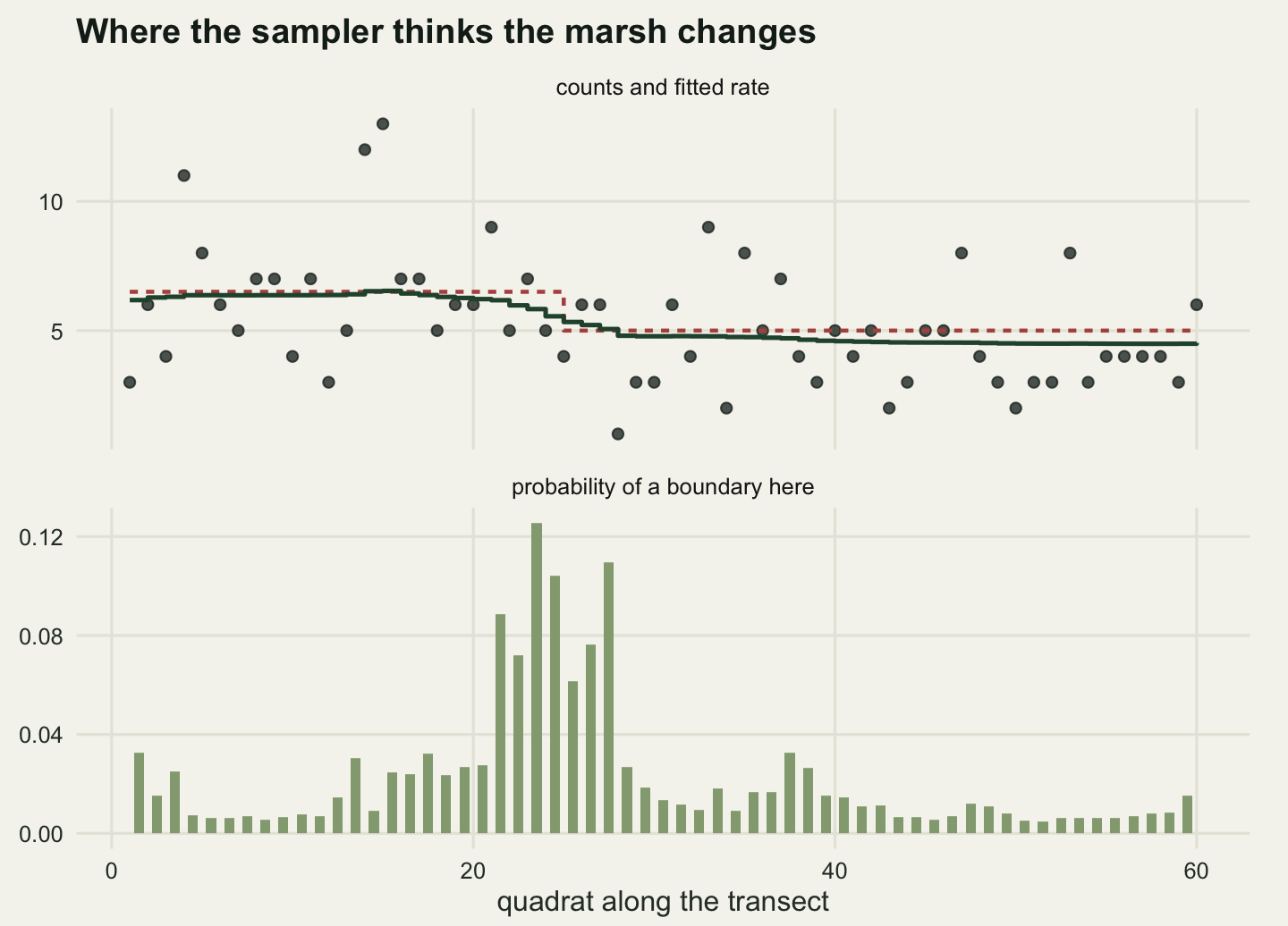
The boundary is not sharply located. Summing the posterior probability over the gaps from 20 to 28 gives 0.6917, so the chain is fairly sure there is a change somewhere in that stretch and has no opinion about where. That is information the model probability alone does not carry, and it comes free from the same chain.

Removing the Jacobian

The Jacobian is one term in a sum of four, it is easy to leave out, and leaving it out does not raise an error, slow the chain down or spoil any diagnostic. Here is what it does instead. The same code runs with jacobian = FALSE, the same data, the same seed, the same split width.

brk_quad <- rj_chain(n_iter, sig_best, 7301, jacobian = FALSE, area = 1, keep = FALSE)
k_brk <- brk_quad$k[-seq_len(n_burn)]
pk_brk <- tabulate(k_brk + 1, k_max + 1) / length(k_brk)
tv_dist <- 0.5 * sum(abs(pk_brk - pk_exact))
tail_exact <- sum(pk_exact[3:4]); tail_brk <- sum(pk_brk[3:4])
print(round(rbind(exact = pk_exact, no_jacobian = pk_brk), 5))

               [,1]    [,2]    [,3]    [,4]
exact       0.08132 0.56751 0.25053 0.10064
no_jacobian 0.40816 0.53904 0.04880 0.00400

print(round(c(birth_acc = brk_quad$birth_acc, death_acc = brk_quad$death_acc,
              switches_per_1000 = 1000 * mean(diff(k_brk) != 0),
              ess_indicator = ess_of(k_brk)), 4))

        birth_acc         death_acc switches_per_1000     ess_indicator 
           0.1278            0.2999          178.7851         5722.3790 

print(round(c(total_variation = tv_dist,
              p_none_exact = pk_exact[1], p_none_broken = pk_brk[1],
              ratio_none = pk_brk[1] / pk_exact[1],
              p_two_or_more_exact = tail_exact, p_two_or_more_broken = tail_brk,
              ratio_tail = tail_exact / tail_brk), 5))

     total_variation         p_none_exact        p_none_broken 
             0.32684              0.08132              0.40816 
          ratio_none  p_two_or_more_exact p_two_or_more_broken 
             5.01917              0.35116              0.05280 
          ratio_tail 
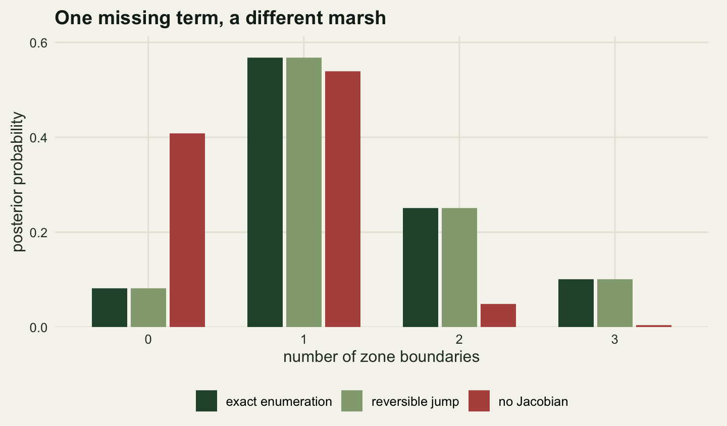
             6.65085 

The broken chain is in perfect health. It accepted 12.78 per cent of births, changed model 178.8 times per thousand iterations, and returned an effective sample size of 5722 for the indicator, in the same range as the correct sampler. No trace looks odd, no acceptance rate is alarming, and no diagnostic in common use would flag it.

The answer it gives is wrong and looks reasonable. It still picks one boundary as the most probable model, at 0.539 against the exact 0.5675, so a reader glancing at the headline would see nothing amiss. Underneath, the probability of no boundary at all has gone from 0.0813 to 0.4082, a factor of 5.02, and the probability of two boundaries or more has fallen from 0.3512 to 0.0528, a factor of 6.65. The total variation distance between the broken posterior and the true one is 0.3268. In words, a study that reported this would say the transect shows at most one zone boundary, when the honest answer gives more than a third of its weight to a finer zonation.

The direction is predictable from the algebra. The omitted factor is \(\lambda_1 \lambda_2 / \lambda\), which for a split into similar halves is close to \(\lambda\) itself, and the posterior mean rate along the transect is 5.301 snails per quadrat. Dropping it therefore divides every birth ratio by something of that order, births are suppressed, deaths are not, and the chain settles on models that are too small.

Now the units. The same broken code is run again with the rate carried as a density per square metre rather than per quadrat, which is a pure reparametrisation: the prior on the implied per-quadrat mean is unchanged, the likelihood is unchanged, and the correct sampler is invariant to it.

ok_m2 <- rj_chain(n_iter, sig_best, 7301, jacobian = TRUE,
                  area = quad_area, keep = FALSE)
brk_m2 <- rj_chain(n_iter, sig_best, 7301, jacobian = FALSE,
                   area = quad_area, keep = FALSE)
pk_ok_m2 <- tabulate(ok_m2$k[-seq_len(n_burn)] + 1, k_max + 1) / (n_iter - n_burn)
pk_brk_m2 <- tabulate(brk_m2$k[-seq_len(n_burn)] + 1, k_max + 1) / (n_iter - n_burn)

print(round(rbind(exact = pk_exact, correct_per_m2 = pk_ok_m2,
                  broken_per_quadrat = pk_brk, broken_per_m2 = pk_brk_m2), 5))

                      [,1]    [,2]    [,3]    [,4]
exact              0.08132 0.56751 0.25053 0.10064
correct_per_m2     0.08162 0.57222 0.24951 0.09665
broken_per_quadrat 0.40816 0.53904 0.04880 0.00400
broken_per_m2      0.74564 0.24898 0.00533 0.00005

print(round(c(correct_max_gap = max(abs(pk_ok_m2 - pk_exact)),
              broken_gap_between_units = max(abs(pk_brk_m2 - pk_brk)),
              quadrats_per_m2 = 1 / quad_area), 5))

         correct_max_gap broken_gap_between_units          quadrats_per_m2 
                 0.00470                  0.33747                  4.00000 

The correct sampler in per-square-metre units lands within 0.0047 of the exact answer at every model size. The broken sampler gives 0.4082 for no boundary when abundance is written per quadrat and 0.7456 when the same abundance is written per square metre. The two runs share a seed, a dataset and a line of source code; the only difference is the unit in which a number is recorded, and the answer moves by 0.3375. That is the concrete form of the dimension argument at the top of the post. A missing Jacobian is not an approximation. It is a statement whose meaning depends on the notebook.

Figure 2: Posterior probability of each number of zone boundaries: the exact value from enumeration, the average of eight reversible jump chains, and the same sampler with the Jacobian removed. The correct chains sit on the exact values to within Monte Carlo error. The broken chain still calls one boundary the most probable model, and is wrong about everything else.

Why the between-model moves are the hard part

Correctness is one problem and mixing is another. A within-model update only has to move a rate a little way; a birth has to invent a whole new parameter and land it somewhere the posterior likes. The dial is \(\sigma_u\), the spread of the split variate. Too small and the two new rates are nearly equal, a proposal the reverse death would almost never have made, so the ratio is killed by the \(1/q(u)\) factor. Too large and one of the new rates is absurd and the likelihood kills it. The sweep runs eleven values over three orders of magnitude.

sig_grid <- c(0.02, 0.05, 0.1, 0.2, 0.4, 0.8, 1.6, 3.2, 6.4, 12.8, 25.6)
n_tune <- 40000L
n_tune_burn <- 4000L

tune_runs <- lapply(sig_grid, function(s)
  rj_chain(n_tune, s, 8800, keep = FALSE))
tune <- do.call(rbind, Map(function(cc, s) {
  kk <- cc$k[-seq_len(n_tune_burn)]
  data.frame(sigma_u = s, birth = cc$birth_acc, death = cc$death_acc,
             within = cc$within_acc, switches = 1000 * mean(diff(kk) != 0),
             ess = ess_of(kk), ess_per_1000 = 1000 * ess_of(kk) / length(kk),
             p_one = tabulate(kk + 1, k_max + 1)[2] / length(kk))
}, tune_runs, sig_grid))
print(round(tune, 4))

   sigma_u  birth  death within switches       ess ess_per_1000  p_one
1     0.02 0.0457 0.0447 0.6364  45.0568  344.9230       9.5812 0.5474
2     0.05 0.1034 0.0996 0.6363 101.8917  885.1346      24.5871 0.5386
3     0.10 0.1808 0.1745 0.6369 178.1716 1999.2771      55.5355 0.5789
4     0.20 0.2648 0.2523 0.6394 257.7849 2464.8909      68.4692 0.5760
5     0.40 0.2934 0.2875 0.6393 291.0081 2347.0009      65.1945 0.5640
6     0.80 0.2624 0.2529 0.6405 257.8961 2669.4349      74.1510 0.5748
7     1.60 0.1911 0.1824 0.6377 187.3385 2177.6451      60.4901 0.5674
8     3.20 0.1122 0.1103 0.6405 111.2809 1139.4258      31.6507 0.5823
9     6.40 0.0618 0.0627 0.6427  61.5295  613.7928      17.0498 0.5899
10   12.80 0.0347 0.0341 0.6388  34.8621  480.9435      13.3595 0.5901
11   25.60 0.0199 0.0192 0.6359  20.1394  195.1499       5.4208 0.5738

best_row <- tune[which.max(tune$ess), ]
worst_row <- tune[nrow(tune), ]
mcse_best <- sqrt(0.25 / best_row$ess)
mcse_worst <- sqrt(0.25 / worst_row$ess)
target_mcse <- 0.001
ess_needed <- 0.25 / target_mcse^2
iters_millions <- ess_needed / (best_row$ess_per_1000 / 1000) / 1e6
print(round(c(best_sigma = best_row$sigma_u, best_birth_acc = best_row$birth,
              worst_sigma = worst_row$sigma_u, worst_birth_acc = worst_row$birth,
              acceptance_ratio = best_row$birth / worst_row$birth,
              ess_ratio = best_row$ess / worst_row$ess,
              mcse_best = mcse_best, mcse_worst = mcse_worst,
              p_one_spread = diff(range(tune$p_one)),
              ess_for_target_mcse = ess_needed,
              million_iterations_for_that = iters_millions), 4))

                 best_sigma              best_birth_acc 
                     0.8000                      0.2624 
                worst_sigma             worst_birth_acc 
                    25.6000                      0.0199 
           acceptance_ratio                   ess_ratio 
                    13.2085                     13.6789 
                  mcse_best                  mcse_worst 
                     0.0097                      0.0358 
               p_one_spread         ess_for_target_mcse 
                     0.0515                 250000.0000 
million_iterations_for_that 
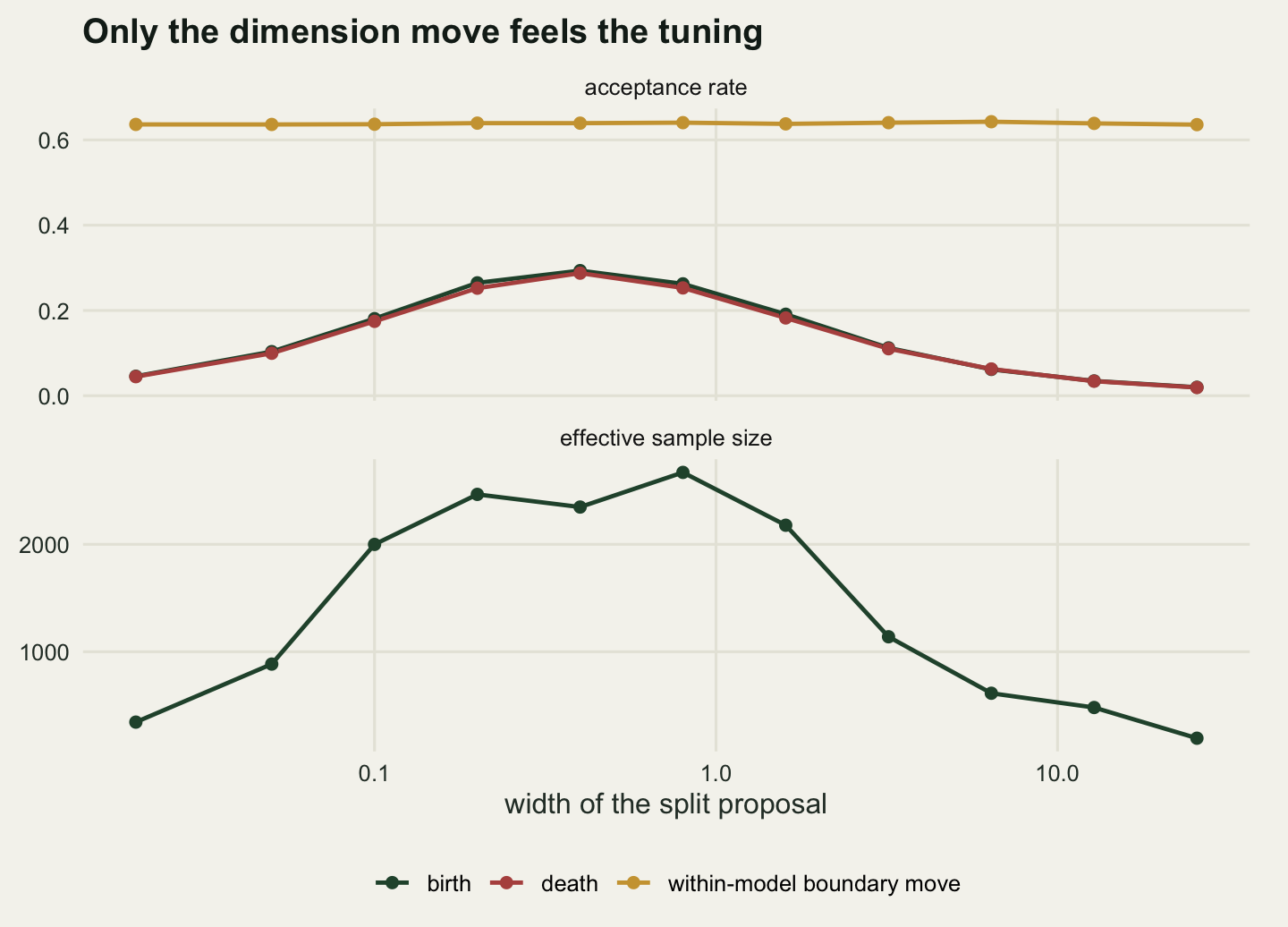
                     3.3715 

Between-model acceptance peaks at 29.34 per cent and falls to 1.99 per cent at the widest split, a factor of 14.77. The within-model boundary move sits at 63.86 per cent throughout and does not care what the split width is, because it is not the move that has to cross between models. That separation is the practical signature of a reversible jump problem: a chain can look well tuned by every within-model measure and still be barely able to change model.

The consequence is in the effective sample size, not in the answer. Across the whole sweep the estimated probability of one boundary stays inside a range of 0.0515, so bad tuning biases nothing; every one of these chains is targeting the right distribution. What it destroys is precision. The best setting reached an effective sample size of 2669 for the model indicator and the worst 195, a factor of 13.68, so the Monte Carlo standard error on a model probability near one half goes from 0.0097 to 0.0358.

That last number governs whether a reported model probability means anything. To pin a probability near one half down to a standard error of 0.001 needs an effective sample size of 250000, which at the best setting measured here would take about 3.37 million iterations. Reporting a posterior model probability to three decimal places from a chain of a few tens of thousands of iterations is reporting Monte Carlo noise.

Figure 3: Between-model acceptance and the effective sample size of the model indicator against the width of the split proposal, on a log axis. The upper panel also shows the within-model boundary move, which is flat: it is unaffected by how the dimension move is tuned. Both between-model curves fall away at either end, and the collapse at the wide end is the more severe.

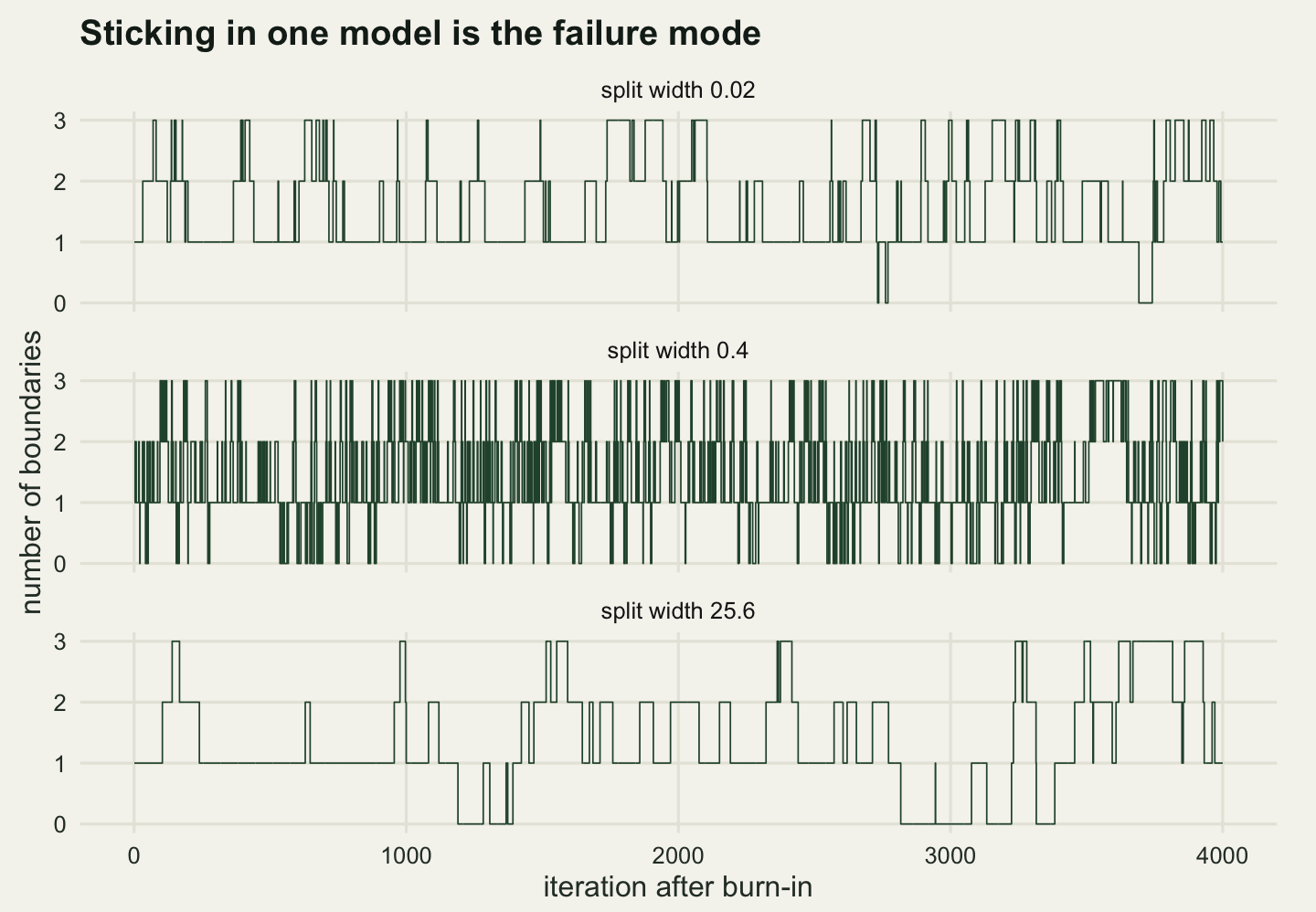
The traces make the same point in a way a summary statistic cannot.

Figure 4: The model indicator over the first four thousand kept iterations at three split widths. The well tuned chain changes model constantly and visits all four sizes. The two badly tuned chains visit the same four sizes and reach the same answer eventually, but they sit in one model for long stretches, so each stretch contributes almost nothing new.

The prior does not wash out

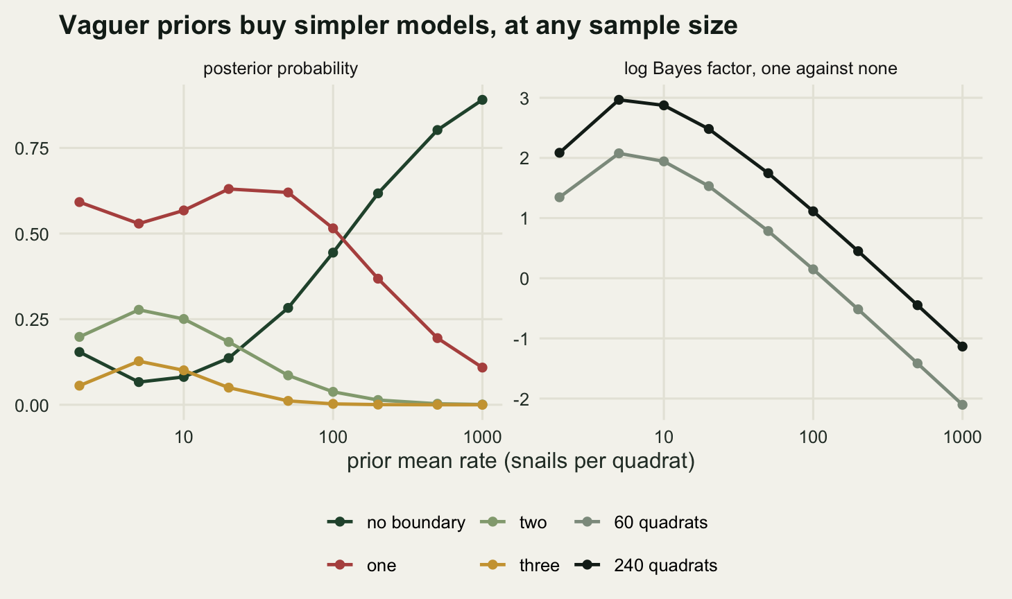
Posterior model probabilities depend on the prior for the parameters in a way that posterior parameter estimates do not. The reason is visible in the closed form above: with shape one, each zone contributes a factor \(b\) to the marginal likelihood, so a model with one more zone carries one more factor of the prior rate. Make the prior vaguer, meaning a smaller \(b\) and a larger prior mean, and the extra zone is charged more. The parameter posterior, meanwhile, barely notices, because the data swamp the prior for a rate that has plenty of quadrats behind it.

Both quantities are computed exactly across a sweep of prior means running from just below the observed mean count to two hundred times it, which spans most of what gets written down as a default.

prior_means <- c(2, 5, 10, 20, 50, 100, 200, 500, 1000)
prior_tab <- do.call(rbind, lapply(prior_means, function(pm) {
  lm_k <- model_lml(rate = 1 / pm)
  pk <- exp(lm_k - log_sum_exp(lm_k))
  data.frame(prior_mean = pm, p0 = pk[1], p1 = pk[2], p2 = pk[3], p3 = pk[4],
             p_two_plus = pk[3] + pk[4], log_bf_10 = lm_k[2] - lm_k[1],
             post_mean_upper = (a_pr + sum(y[seq_len(tau_true)])) /
               (1 / pm + tau_true))
}))
print(round(prior_tab, 5))

  prior_mean      p0      p1      p2      p3 p_two_plus log_bf_10
1          2 0.15406 0.59191 0.19825 0.05578    0.25403   1.34600
2          5 0.06631 0.52903 0.27739 0.12727    0.40466   2.07669
3         10 0.08132 0.56751 0.25053 0.10064    0.35116   1.94286
4         20 0.13628 0.63017 0.18350 0.05005    0.23355   1.53128
5         50 0.28289 0.61993 0.08581 0.01136    0.09717   0.78454
6        100 0.44432 0.51520 0.03781 0.00268    0.04049   0.14801
7        200 0.61737 0.36821 0.01392 0.00051    0.01443  -0.51681
8        500 0.80228 0.19468 0.00300 0.00004    0.00304  -1.41610
9       1000 0.89050 0.10866 0.00084 0.00001    0.00085  -2.10358
  post_mean_upper
1         6.48980
2         6.57025
3         6.59751
4         6.61123
5         6.61948
6         6.62224
7         6.62362
8         6.62445
9         6.62472

par_spread <- diff(range(prior_tab$post_mean_upper)) / mean(prior_tab$post_mean_upper)
print(round(c(p_none_low = min(prior_tab$p0), p_none_high = max(prior_tab$p0),
              p_one_range = diff(range(prior_tab$p1)),
              p_two_plus_low = min(prior_tab$p_two_plus),
              p_two_plus_high = max(prior_tab$p_two_plus),
              parameter_relative_range = par_spread), 5))

              p_none_low              p_none_high              p_one_range 
                 0.06631                  0.89050                  0.52151 
          p_two_plus_low          p_two_plus_high parameter_relative_range 
                 0.00085                  0.40466                  0.02045 

Across that sweep the probability of no boundary at all runs from 0.0663 to 0.8905, the probability of one boundary moves over a range of 0.5215, and the probability of two boundaries or more spans 0.00085 to 0.4047. Over the same sweep the posterior mean rate in the upper part of the transect moves by 2.045 per cent of its own value. The parameter is settled by the data and the model probability is not.

The dependence does not fade with more data. That is the Jeffreys-Lindley paradox, named for Lindley (1957), and in this model it has an exact form: in the diffuse limit each extra zone contributes exactly one factor of the prior rate, so doubling the prior mean halves the Bayes factor for the extra zone whatever the data say. A transect four times as long, generated from the same step function, shows the same slope.

set.seed(20260804)
n_long <- 240L
tau_long <- 96L
y_long <- rpois(n_long, dens_true[ifelse(seq_len(n_long) <= tau_long, 1L, 2L)])
cs_long <- c(0, cumsum(y_long))
cf_long <- c(0, cumsum(lgamma(y_long + 1)))

seg_lml_long <- function(i, j, rate) {
  ss <- cs_long[j + 1] - cs_long[i]; mm <- j - i + 1
  a_pr * log(rate) - lgamma(a_pr) + lgamma(a_pr + ss) -
    (a_pr + ss) * log(rate + mm) - (cf_long[j + 1] - cf_long[i])
}

long_tab <- do.call(rbind, lapply(prior_means, function(pm) {
  lm_k <- model_lml(rate = 1 / pm, nn = n_long, lml_fun = seg_lml_long)
  pk <- exp(lm_k - log_sum_exp(lm_k))
  data.frame(prior_mean = pm, p0 = pk[1], p1 = pk[2], p_two_plus = pk[3] + pk[4],
             log_bf_10 = lm_k[2] - lm_k[1])
}))
print(round(long_tab, 5))

  prior_mean      p0      p1 p_two_plus log_bf_10
1          2 0.07930 0.63852    0.28217   2.08586
2          5 0.02706 0.52553    0.44741   2.96619
3         10 0.03240 0.57361    0.39399   2.87389
4         20 0.05593 0.66892    0.27515   2.48156
5         50 0.12925 0.74072    0.13003   1.74589
6        100 0.23185 0.70561    0.06254   1.11297
7        200 0.37910 0.59451    0.02640   0.44994
8        500 0.60603 0.38709    0.00687  -0.44827
9       1000 0.75520 0.24264    0.00215  -1.13540

tail_sel <- prior_means >= 100
slope_theory <- -1
log_pm <- log(prior_means[tail_sel])
slope_short <- unname(coef(lm(prior_tab$log_bf_10[tail_sel] ~ log_pm))[2])
slope_long <- unname(coef(lm(long_tab$log_bf_10[tail_sel] ~ log_pm))[2])
bf_gain <- mean(long_tab$log_bf_10 - prior_tab$log_bf_10)
prior_factor <- exp(bf_gain / abs(slope_short))
print(round(c(slope_60_quadrats = slope_short, slope_240_quadrats = slope_long,
              theory = slope_theory, mean_log_bf_gain = bf_gain,
              prior_factor_that_cancels_it = prior_factor,
              long_two_plus_low = min(long_tab$p_two_plus),
              long_two_plus_high = max(long_tab$p_two_plus),
              long_two_plus_ratio = max(long_tab$p_two_plus) /
                min(long_tab$p_two_plus)), 5))

           slope_60_quadrats           slope_240_quadrats 
                    -0.97834                     -0.97698 
                      theory             mean_log_bf_gain 
                    -1.00000                      0.92664 
prior_factor_that_cancels_it            long_two_plus_low 
                     2.57836                      0.00215 
          long_two_plus_high          long_two_plus_ratio 
                     0.44741                    207.67644 

Regressing the log Bayes factor for one boundary against none on the log prior mean, over the diffuse part of the sweep, gives a slope of -0.9783 on the sixty quadrat transect and -0.977 on the two hundred and forty quadrat one, against a theoretical -1. Quadrupling the data changed the slope by 0.0014.

What the extra data did buy is evidence. The log Bayes factor for one boundary rose by 0.9266 on average across the prior sweep, uniformly at every prior. Set that against the slope and the exchange rate is blunt: making the prior mean 2.58 times vaguer gives back everything the extra one hundred and eighty quadrats earned. And the finer question is no better settled than before, the probability of two boundaries or more on the long transect still ranging from 0.00215 to 0.4474 across the same priors, a factor of 207.68.

A default vague prior is therefore a strong statement about model choice, and the strength does not decay. Barker and Link (2013) make the point that reversible jump output is only as meaningful as the priors that went into it, and this is the mechanism.

Figure 5: Left: exact posterior probability of each number of boundaries against the prior mean for a zone rate, on a log axis. Right: log Bayes factor for one boundary against none, for the sixty quadrat transect and one four times longer, over the same priors. The two lines are parallel with slope near minus one, so the prior dependence is unchanged by quadrupling the data.

The honest limit

Reversible jump is correct and it is general. It is also the option most likely to be implemented wrongly, and the failure is silent. The broken chain in this post produced a 12.78 per cent birth acceptance rate, an effective sample size of 5722, traces that look identical to the correct ones, and a posterior that agrees with the truth about which model is most probable while being wrong by a factor of 6.65 about everything else. There is no convergence diagnostic for a wrong target. The only check that worked here was comparing against an answer computed a different way, and that check is available precisely when the sampler is least necessary.

Which is the second limit, and it applies to this post’s own example. The rates are conjugate and the positions are discrete, so the exact posterior over models is a finite sum that a dynamic program evaluates in a fraction of a second: nothing here needed a sampler at all. For a small fixed set of models the same is often true in practice. Estimating each marginal likelihood separately, by bridge sampling or by a Laplace approximation, gives numbers that can be checked one at a time and recomputed when a prior changes, and comparing predictive scores with WAIC or PSIS-LOO avoids model probability altogether. Reversible jump earns its place when the model space is too large to enumerate: an unknown number of mixture components in the sense of Richardson and Green (1997), a variable set of covariates, the capture-recapture model spaces of King and Brooks (2002). Lunn, Best and Whittaker (2009) show how far the algorithm can be made generic inside a graphical modelling framework.

The third limit is the tuning. The split proposal was hand-built for this model and it took a sweep over three orders of magnitude to find its useful range. Brooks, Giudici and Roberts (2003) give constructions that avoid guessing and the review by Hastie and Green (2012) is the place to start, but there is no default that works, and the effective sample size of the model indicator is what has to be reported. Here it ranged from 195 to 2669 out of 36000 draws.

The last limit is not computational. A posterior probability over models is a statement about a set that is assumed to contain the truth, and here that assumption holds by construction. A real saltmarsh does not have step-function zonation: densities change over metres rather than at a line, and the number of boundaries in a piecewise-constant fit is then a property of the approximation rather than of the marsh. The probabilities remain well defined and they stop being about the ecology.

Where to go next

The natural companion is the same problem attacked from the other end: estimate each model’s marginal likelihood separately and form the Bayes factors by hand, which is what bridge sampling does, and compare the answers against the enumeration used here. The other direction is the product-space reformulation of Barker and Link (2013), which turns the same computation into a Gibbs sampler over a fixed-dimension state and moves the Jacobian out of the code and into the model specification. Whether that is a genuine simplification or a relocation of the same difficulty has a measurable answer, on this transect.

References

Green PJ 1995 Biometrika 82(4):711-732 (10.1093/biomet/82.4.711)

Richardson S, Green PJ 1997 Journal of the Royal Statistical Society B 59(4):731-792 (10.1111/1467-9868.00095)

Brooks SP, Giudici P, Roberts GO 2003 Journal of the Royal Statistical Society B 65(1):3-39 (10.1111/1467-9868.03711)

Hastie DI, Green PJ 2012 Statistica Neerlandica 66(3):309-338 (10.1111/j.1467-9574.2012.00516.x)

Lindley DV 1957 Biometrika 44(1-2):187-192 (10.1093/biomet/44.1-2.187)

King R, Brooks SP 2002 Biometrics 58(4):841-851 (10.1111/j.0006-341X.2002.00841.x)

Barker RJ, Link WA 2013 The American Statistician 67(3):150-156 (10.1080/00031305.2013.791644)

Lunn DJ, Best N, Whittaker JC 2009 Statistics and Computing 19(4):395-408 (10.1007/s11222-008-9100-0)

Related tutorials

• Metropolis-Hastings from scratch
• Bridge sampling for marginal likelihoods
• Bayesian model comparison: WAIC, LOO, DIC
• How many states in a movement HMM?