library(ggplot2)

te_pal <- list(forest = "#275139", green = "#2f8f63", sage = "#93a87f",
               clay = "#b5534e", gold = "#cda23f", line = "#dad9ca",
               ink = "#16241d", paper = "#f5f4ee")

theme_te <- function() {
  theme_minimal(base_size = 12) +
    theme(panel.grid.minor = element_blank(),
          panel.grid.major = element_line(colour = "#e7e6dc"),
          plot.background = element_rect(fill = "#f5f4ee", colour = NA),
          panel.background = element_rect(fill = "#f5f4ee", colour = NA),
          plot.title = element_text(face = "bold", colour = te_pal$ink),
          axis.title = element_text(colour = "#2c3a31"),
          axis.text = element_text(colour = "#2c3a31"))
}Bridge sampling for marginal likelihoods
R
Bayesian statistics
MCMC
model selection
ecology tutorial
Estimating a marginal likelihood in base R: the harmonic mean measured against an exact answer, the bridge identity derived, and three ecological posteriors.
A chalk stream survey, done over three weeks in May. Fifteen riffles, three kick samples in each, so forty-five samples in all. Every sample was sorted, the nymphs of one mayfly were counted, the whole sample was dried and weighed, and the percentage of the streambed covered by fine sediment was recorded at each kick point. Thirty-six of the nymphs went into a separate tube and had their body length measured, because the recorder suspected two cohorts were present.
Three questions come out of that, and all three are model comparisons. Does the count respond to fine sediment, or is a single mean enough? Does the sample dry mass vary between riffles by more than the within-riffle noise, or can the riffles be pooled? Are those thirty-six body lengths one cohort or two? A Bayes factor answers each of them, and a Bayes factor is a ratio of two marginal likelihoods: the probability of the data under a model, with the parameters integrated out against the prior rather than fixed at any estimate.
That integral is the problem. Posterior draws do not give it, because the posterior is what you get after dividing by it. There is a long tradition of estimating it from posterior draws anyway, and most of that tradition does not work. This post implements the estimators that do not work and measures how badly, then derives bridge sampling and measures that against an exact answer on three targets: one well behaved, two of them the shapes that break everything else.
The positioning matters here because one neighbouring post is close. The Laplace approximation in R already computes marginal likelihoods, checks them against exact values, and documents three ways the approximation fails: a skewed posterior, a posterior with two modes, and a variance component whose mass piles against a boundary. This post is what to do about those three failures. The Laplace approximation is not rebuilt below; it is used as one of the five estimators in the comparison, and the two hard targets are chosen to be the shapes it failed on, so the question is whether bridge sampling survives them. It survives two of the three, and the third it inherits from the sampler.
Bayesian model comparison: WAIC, LOO, DIC answers a different question from the same posterior draws. A predictive score estimates out-of-sample loss for the model as fitted; a marginal likelihood is the prior predictive probability of the data actually seen, a statement about the model together with its prior. The two can rank the same candidates differently, and the last section measures how far apart they can be pulled by nothing but a change of prior scale. If the question is which model predicts better, use the predictive score and skip this post.
The checking discipline comes from Checking a Bayesian computation: compare against an exact benchmark where one exists, report a Monte Carlo error next to every number, and treat a reported standard error as a claim that itself needs testing. Every target below is small enough to integrate exactly, so every estimator gets a verdict rather than a plausibility argument. The same-day sibling Reversible jump MCMC from scratch reaches posterior model probabilities without ever computing a marginal likelihood; prefer that route when there are many models and a jump proposal between them is easy to write, and this one when the models are few, unrelated in shape, or already fitted separately.
An integral over the prior, not the posterior
Write \(p(y \mid \theta)\) for the likelihood and \(p(\theta)\) for the prior, so that
\[p(y) \;=\; \int p(y \mid \theta)\, p(\theta)\, \mathrm{d}\theta\]
and the posterior is \(p(\theta \mid y) = p(y \mid \theta) p(\theta) / p(y)\). Two things follow. The integral is taken against the prior, so it is sensitive to parts of the parameter space the data rule out, which the posterior is not. And the unnormalised posterior \(p^{*}(\theta) = p(y \mid \theta) p(\theta)\) is the only object a sampler evaluates, so a chain that has run perfectly still carries no direct information about the constant it was divided by.
logsumexp <- function(v) { mx <- max(v); mx + log(sum(exp(v - mx))) }
lse2 <- function(a, b) { mx <- pmax(a, b); mx + log(exp(a - mx) + exp(b - mx)) }
fmt <- function(x, d = 4) formatC(x, format = "f", digits = d)
sci <- function(x, d = 2) formatC(x, format = "e", digits = d)

set.seed(20260803)
n_rif <- 15; n_sub <- 3; n_kick <- n_rif * n_sub
fines <- as.vector(scale(runif(n_kick, 5, 60)))
y_kick <- rpois(n_kick, exp(1.75 - 0.55 * fines))
rif_id <- rep(seq_len(n_rif), each = n_sub)

set.seed(20260807)
lmass <- rep(rnorm(n_rif, 0, 0.12), each = n_sub) + rnorm(n_kick, log(1.8), 0.5)

set.seed(20260804)
n_ind <- 36
blen <- ifelse(rbinom(n_ind, 1, 0.5) == 1, 1.5, -1.5) + rnorm(n_ind, 0, 1)

print(c(riffles = n_rif, subsamples = n_sub, kick_samples = n_kick,
        total_nymphs = sum(y_kick), empty_samples = sum(y_kick == 0),
        largest_sample = max(y_kick), nymphs_measured = n_ind))
riffles subsamples kick_samples total_nymphs empty_samples
15 3 45 297 0
largest_sample nymphs_measured
16 36 print(round(c(mean_count = mean(y_kick), mean_log_mass = mean(lmass),
sd_log_mass = sd(lmass)), 4)) mean_count mean_log_mass sd_log_mass
6.6000 0.5410 0.5044 The survey yields 297 nymphs across 45 samples, a mean of 6.60 per sample, 0 empty samples and a largest catch of 16. The first target is a Poisson regression of those counts on standardised fine sediment cover, with an independent normal prior on each of the two coefficients. It has an interior mode, mild curvature and nothing unusual about it, which is what a baseline needs.
Because the likelihood depends on the coefficients only through three sufficient statistics, the two-dimensional integral can be evaluated on a grid at negligible cost, and calling a grid answer exact needs a check: the grid below is computed over eight posterior standard deviations at 401 points a side, twelve at 1201 and eighteen at 1601.
pri_sd <- c(2, 1)
S_y <- sum(y_kick); S_xy <- sum(y_kick * fines); c_lg <- sum(lgamma(y_kick + 1))

llik1 <- function(bm) {
  sx <- colSums(exp(outer(fines, bm[, 2])))
  bm[, 1] * S_y + bm[, 2] * S_xy - exp(bm[, 1]) * sx - c_lg
}
lup1 <- function(bm) llik1(bm) +
  dnorm(bm[, 1], 0, pri_sd[1], log = TRUE) + dnorm(bm[, 2], 0, pri_sd[2], log = TRUE)
rpri1 <- function(n_s) cbind(rnorm(n_s, 0, pri_sd[1]), rnorm(n_s, 0, pri_sd[2]))

laplace_at <- function(lup, start) {
  nf <- function(bv) -lup(matrix(bv, nrow = 1))
  o <- optim(start, nf, method = "BFGS", control = list(reltol = 1e-14))
  Hm <- optimHess(o$par, nf)
  list(mode = o$par, V = solve(Hm),
       logml = -o$value + 0.5 * length(start) * log(2 * pi) -
         0.5 * as.numeric(determinant(Hm)$modulus))
}
lap1 <- laplace_at(lup1, c(0, 0))

pois_grid <- function(yv, xv, psd, ng, hw = 12) {
  Syl <- sum(yv); Sxyl <- sum(yv * xv); clgl <- sum(lgamma(yv + 1))
  nf <- function(bv) -(bv[1] * Syl + bv[2] * Sxyl -
    exp(bv[1]) * sum(exp(bv[2] * xv)) - clgl +
    dnorm(bv[1], 0, psd[1], log = TRUE) + dnorm(bv[2], 0, psd[2], log = TRUE))
  o <- optim(c(0, 0), nf, method = "BFGS", control = list(reltol = 1e-14))
  s0 <- sqrt(diag(solve(optimHess(o$par, nf))))
  g0 <- seq(o$par[1] - hw * s0[1], o$par[1] + hw * s0[1], length.out = ng)
  g1 <- seq(o$par[2] - hw * s0[2], o$par[2] + hw * s0[2], length.out = ng)
  sx <- vapply(g1, function(b) sum(exp(b * xv)), numeric(1))
  lp <- outer(g0 * Syl, g1 * Sxyl, "+") - outer(exp(g0), sx, "*") - clgl +
    outer(dnorm(g0, 0, psd[1], log = TRUE),
          dnorm(g1, 0, psd[2], log = TRUE), "+")
  list(g0 = g0, g1 = g1, lp = lp,
       logml = logsumexp(as.vector(lp)) + log(diff(g0)[1]) + log(diff(g1)[1]))
}
exact1 <- pois_grid(y_kick, fines, pri_sd, 1201)$logml
print(round(c(mode_intercept = lap1$mode[1], mode_slope = lap1$mode[2],
              sd_intercept = sqrt(lap1$V[1, 1]), sd_slope = sqrt(lap1$V[2, 2])), 4))
mode_intercept mode_slope sd_intercept sd_slope
1.7526 -0.5392 0.0661 0.0668 print(c(coarse = pois_grid(y_kick, fines, pri_sd, 401, 8)$logml, fine = exact1,
wide = pois_grid(y_kick, fines, pri_sd, 1601, 18)$logml)) coarse fine wide
-98.1541 -98.1541 -98.1541 print(round(c(exact_log_ml = exact1, laplace_log_ml = lap1$logml,
laplace_error = lap1$logml - exact1), 6)) exact_log_ml laplace_log_ml laplace_error
-98.154100 -98.154874 -0.000774 The three grids agree to twelve decimal places, so -98.154100 is the integral and not the grid. The Laplace approximation, which is one optimisation and one determinant, comes in 7.74e-04 below it. On this target there is nothing to fix.
Two estimators that do not work
Both classical estimators are one line, which is most of why they persist. The arithmetic mean estimator draws from the prior and averages the likelihood, because the marginal likelihood is a prior expectation by definition. The harmonic mean estimator (Newton and Raftery 1994) uses posterior draws and takes the harmonic mean of the likelihood, which is unbiased for the reciprocal of the marginal likelihood and needs no proposal at all.
Neither is asserted to fail below. Both are run twenty times on the same target, and the spread across those runs is the measurement.
rwm <- function(lup, start, n_iter, Cprop, seed, flip = FALSE) {
  set.seed(seed)
  d <- length(start); out <- matrix(NA_real_, n_iter, d)
  cur <- start; lcur <- lup(matrix(cur, nrow = 1)); n_acc <- 0
  Ch <- chol(Cprop)
  for (i in seq_len(n_iter)) {
    prop <- cur + as.vector(crossprod(Ch, rnorm(d)))
    if (flip && runif(1) < 0.5) prop <- -prop
    lpv <- lup(matrix(prop, nrow = 1))
    if (log(runif(1)) < lpv - lcur) { cur <- prop; lcur <- lpv; n_acc <- n_acc + 1 }
    out[i, ] <- cur
  }
  list(draws = out, acc = n_acc / n_iter)
}
thin_of <- function(ch, warm, by)
  ch$draws[seq(warm + 1, nrow(ch$draws), by = by), , drop = FALSE]

n_rep <- 20
ch1 <- rwm(lup1, lap1$mode, 44000, lap1$V * 2.4^2 / 2, 4101)
post1 <- thin_of(ch1, 4000, 4)
rep1 <- lapply(seq_len(n_rep), function(r)
  thin_of(rwm(lup1, lap1$mode, 44000, lap1$V * 2.4^2 / 2, 5200 + r), 4000, 4))
n_draw <- nrow(post1)
print(round(c(iterations = 44000, acceptance = ch1$acc, kept_draws = n_draw,
              lag1_intercept = cor(post1[-1, 1], post1[-n_draw, 1]),
              lag1_slope = cor(post1[-1, 2], post1[-n_draw, 2]),
              replicate_samples = n_rep), 4))
iterations acceptance kept_draws lag1_intercept
4.400e+04 3.523e-01 1.000e+04 3.376e-01
lag1_slope replicate_samples
3.428e-01 2.000e+01 The sampler is a random walk Metropolis loop with its proposal covariance taken from the Laplace approximation and scaled by the usual \(2.4^2/d\). Acceptance is 0.352, and thinning by four leaves 10000 draws with a lag one autocorrelation of 0.343 on the slope. Twenty independent replicates of that run supply the Monte Carlo error for everything below.
am_est <- function(llik, rpri, n_s) {
  bm <- rpri(n_s); lw <- llik(bm)
  list(logml = logsumexp(lw) - log(n_s), top = exp(max(lw) - logsumexp(lw)))
}
hm_est <- function(llik, pd) log(nrow(pd)) - logsumexp(-llik(pd))

set.seed(20260808)
am1 <- t(vapply(seq_len(n_rep), function(r) unlist(am_est(llik1, rpri1, n_draw)),
                numeric(2)))
hm1 <- vapply(rep1, function(pd) hm_est(llik1, pd), numeric(1))
print(round(c(exact = exact1, am_mean = mean(am1[, 1]), am_sd = sd(am1[, 1]),
              am_lowest = min(am1[, 1]), am_highest = max(am1[, 1]),
              am_largest_share = mean(am1[, 2])), 4))
exact am_mean am_sd am_lowest
-98.1541 -98.1373 0.2086 -98.4508
am_highest am_largest_share
-97.8137 0.0817 print(round(c(hm_mean = mean(hm1), hm_sd = sd(hm1), hm_lowest = min(hm1),
hm_highest = max(hm1), hm_bias = mean(hm1) - exact1), 4)) hm_mean hm_sd hm_lowest hm_highest hm_bias
-93.8384 0.3886 -95.1434 -93.4010 4.3157 The arithmetic mean is not biased in any serious way: over twenty runs it averages -98.137 against an exact -98.154. What it has is variance, a standard deviation of 0.209 log units across runs and a spread from -98.451 to -97.814. The reason is in the last number: on average a single prior draw carries 8.2 per cent of the whole sum, out of 10000 of them. The prior standard deviations are 2 and 1 against posterior standard deviations near 0.07, so the posterior occupies about two tenths of a per cent of the prior volume and almost every draw lands where the likelihood is negligible. Add two more parameters, or widen the prior, and the estimator stops working entirely.
The harmonic mean is worse in a different way. It averages -93.838 against -98.154, a bias of 4.316 log units, with a standard deviation of 0.389 and a range from -95.143 to -93.401. Every one of the twenty runs is above the truth. The mechanism is that \(1/p(y \mid \theta)\) has infinite variance under the posterior for most models: the estimate is dominated by whichever draw sat furthest into the low-likelihood tail, rare huge values pull it down, and between those events it drifts upward. That is not a small-sample problem: the figure two sections below grows the sample and separates an estimator that is merely noisy from one that is not converging at all.
Importance sampling, and the warning it comes with
The honest middle step is importance sampling with a proposal fitted to the posterior rather than to the prior. Draw \(\theta_j\) from a density \(g\) that approximates the posterior, and average the ratio:
\[\hat{p}(y) \;=\; \frac{1}{N}\sum_{j=1}^{N} \frac{p^{*}(\theta_j)}{g(\theta_j)}, \qquad \theta_j \sim g\]
The proposal used throughout is a multivariate normal fitted to the posterior draws themselves. Fitting it to the same draws it will be scored against would reuse the sample, so the draws are split in half: the first half fits the proposal, the second half goes into the estimator.
mvn_logd <- function(bm, mu, Sig) {
  L <- chol(Sig)
  z <- backsolve(L, t(bm) - mu, transpose = TRUE)
  -0.5 * colSums(z^2) - sum(log(diag(L))) - 0.5 * length(mu) * log(2 * pi)
}
mvn_draw <- function(n_s, mu, Sig)
  t(mu + t(matrix(rnorm(n_s * length(mu)), n_s) %*% chol(Sig)))

log_ratios <- function(lup, pd, seed, infl = 1, shift = 0) {
  h <- floor(nrow(pd) / 2)
  fitd <- pd[seq_len(h), , drop = FALSE]; used <- pd[-seq_len(h), , drop = FALSE]
  mu <- colMeans(fitd) + shift * sqrt(diag(cov(fitd)))
  Sig <- cov(fitd) * infl
  set.seed(seed)
  qd <- mvn_draw(nrow(used), mu, Sig)
  list(l1 = lup(used) - mvn_logd(used, mu, Sig),
       l2 = lup(qd) - mvn_logd(qd, mu, Sig))
}
is_est <- function(lr) {
  wv <- exp(lr$l2 - max(lr$l2))
  list(logml = logsumexp(lr$l2) - log(length(lr$l2)),
       ess = sum(wv)^2 / sum(wv^2), top = max(wv) / sum(wv))
}
lr1 <- log_ratios(lup1, post1, 6001)
isr <- is_est(lr1)
print(round(c(is_estimate = isr$logml, is_error = isr$logml - exact1,
              proposal_draws = length(lr1$l2), weight_ess = isr$ess,
              largest_weight_share = isr$top), 6))
is_estimate is_error proposal_draws
-98.15436 -0.00026 5000.00000
weight_ess largest_weight_share
4965.43189 0.00047 The estimate is -98.15436 against an exact -98.15410, an error of 2.60e-04. The diagnostic that says whether to believe it is the effective sample size of the weights, \((\sum w)^2 / \sum w^2\), which is 4965 out of 5000 draws, together with the share of the total carried by the single largest weight, 0.047 per cent. Both say the weights are nearly uniform, which is what a proposal matched to a near-Gaussian posterior should give. When the effective sample size collapses to a few dozen, as it does later in this post, the estimate is a lottery and the diagnostic is the only thing that says so.
The bridge identity
Bridge sampling (Meng and Wong 1996) starts from an identity that holds for any function \(h\), provided the integral in it is finite and non-zero. Write \(p^{*}(\theta)\) for the unnormalised posterior, \(c = \int p^{*}\) for the marginal likelihood, and \(g\) for a normalised proposal. Then
\[\mathbb{E}_{g}\!\left[h(\theta)\, p^{*}(\theta)\right] \;=\; \int h\, p^{*} g \,\mathrm{d}\theta \;=\; c \int h\, g\, \frac{p^{*}}{c}\,\mathrm{d}\theta \;=\; c\; \mathbb{E}_{p}\!\left[h(\theta)\, g(\theta)\right]\]
and therefore
\[c \;=\; \frac{\mathbb{E}_{g}\left[h(\theta) p^{*}(\theta)\right]} {\mathbb{E}_{p}\left[h(\theta) g(\theta)\right]}\]
with the numerator estimated from proposal draws and the denominator from posterior draws. That is the whole trick: the second expectation uses the draws you have, and neither needs the constant being sought.
Every estimator above is this identity with a particular \(h\). Take \(h = 1/g\): the numerator becomes \(\mathbb{E}_{g}[p^{*}/g]\) and the denominator becomes one, which is importance sampling. Take \(h = 1/p^{*}\): the numerator is one and the denominator is \(\mathbb{E}_{p}[g/p^{*}]\), the reciprocal importance sampling estimator of Gelfand and Dey (1994). Now set \(g\) to the prior. Importance sampling becomes \(\mathbb{E}_{\text{prior}}[p(y \mid \theta)]\), the arithmetic mean estimator, and reciprocal importance sampling becomes \(1 / \mathbb{E}_{p}[1/p(y \mid \theta)]\), the harmonic mean. Four estimators, one identity, two choices.
The \(h\) that minimises the relative mean squared error is derived in Meng and Wong (1996):
\[h(\theta) \;\propto\; \frac{1}{s_1 p^{*}(\theta) + s_2\, c\, g(\theta)}, \qquad s_1 = \frac{N_1}{N_1 + N_2},\; s_2 = \frac{N_2}{N_1 + N_2}\]
with \(N_1\) posterior draws and \(N_2\) proposal draws. It contains \(c\), the unknown, so the estimator is a fixed point: substitute a current guess, compute a new estimate, repeat. Gelman and Meng (1998) place this in the wider family of path sampling identities, and Gronau et al (2017) give the tutorial treatment and the practical recipe. The scheme is fifteen lines, all of it on the log scale because \(p^{*}\) here is of order \(e^{-98}\).
bridge_est <- function(l1, l2, lc0 = 0, tol = 1e-10, maxit = 200) {
  n1 <- length(l1); n2 <- length(l2)
  w1 <- log(n1 / (n1 + n2)); w2 <- log(n2 / (n1 + n2))
  lc <- lc0; path <- lc
  for (it in seq_len(maxit)) {
    lnew <- (logsumexp(l2 - lse2(w1 + l2, w2 + lc)) - log(n2)) -
      (logsumexp(-lse2(w1 + l1, w2 + lc)) - log(n1))
    path <- c(path, lnew)
    done <- abs(lnew - lc) < tol
    lc <- lnew
    if (done) break
  }
  f1 <- exp(l2 - lse2(w1 + l2, w2 + lc))
  f2 <- exp(-lse2(w1 + l1, w2 + lc))
  list(logml = lc, iter = it, path = path,
       re = sqrt(var(f1) / mean(f1)^2 / n2 + var(f2) / mean(f2)^2 / n1))
}
both_est <- function(lup, pd, seed, infl = 1, shift = 0) {
  lr <- log_ratios(lup, pd, seed, infl, shift)
  iv <- is_est(lr); br <- bridge_est(lr$l1, lr$l2)
  list(is = iv$logml, ess = iv$ess, top = iv$top, bridge = br$logml,
       re = br$re, iter = br$iter)
}
The two inputs are the log ratios \(\log p^{*} - \log g\) at the posterior draws and at the proposal draws. The re element is the relative error of Fruehwirth-Schnatter (2004), built from the two sets of terms the iteration already computes, and it is the standard error the method reports about itself. It assumes the posterior draws are independent; with an autocorrelated chain the first term has to be inflated by the integrated autocorrelation time, which is why the chains here are thinned. The fixed point can be started anywhere, and where it starts is worth seeing.
is_v <- logsumexp(lr1$l2) - log(length(lr1$l2))
ri_v <- log(length(lr1$l1)) - logsumexp(-lr1$l1)
from_hi <- bridge_est(lr1$l1, lr1$l2, lc0 = 0)
from_lo <- bridge_est(lr1$l1, lr1$l2, lc0 = -1e6)
print(round(c(importance_sampling = is_v, reciprocal_is = ri_v,
              first_iterate_from_above = from_hi$path[2],
              first_iterate_from_below = from_lo$path[2],
              gap_above = from_hi$path[2] - is_v,
              gap_below = from_lo$path[2] - ri_v), 8))
importance_sampling reciprocal_is first_iterate_from_above
-98.15436 -98.15507 -98.15436
first_iterate_from_below gap_above gap_below
-98.15507 0.00000 0.00000 print(round(c(converged_from_above = from_hi$logml,
converged_from_below = from_lo$logml, exact = exact1,
bridge_error = from_hi$logml - exact1, reported_re = from_hi$re,
iterations = from_hi$iter), 6))converged_from_above converged_from_below exact
-98.155051 -98.155051 -98.154100
bridge_error reported_re iterations
-0.000951 0.000776 4.000000 print(round(from_hi$path[1:5], 5))[1] 0.00000 -98.15436 -98.15505 -98.15505 -98.15505Start the iteration at \(c = 1\), which is 98 log units too large, and the first iterate is the importance sampling estimate to the last bit: the gap is 0. Start it at effectively \(c = 0\) and the first iterate is the reciprocal importance sampling estimate, again exactly. The two special cases are the two ends of the iteration and the fixed point sits between them. Both runs converge to -98.15505 in 4 iterations, an error of 9.51e-04 against an exact -98.15410, with a reported relative error of 7.76e-04.
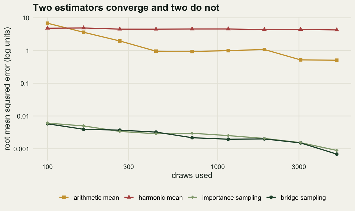
rm_at <- function(nm, s) tr_sum$rmse[tr_sum$estimator == nm & tr_sum$draws == s]
print(round(c(draws_low = min(chk), draws_high = max(chk),
              harmonic_low = rm_at("harmonic mean", min(chk)),
              harmonic_high = rm_at("harmonic mean", max(chk)),
              arithmetic_low = rm_at("arithmetic mean", min(chk)),
              arithmetic_high = rm_at("arithmetic mean", max(chk)),
              bridge_low = rm_at("bridge sampling", min(chk)),
              bridge_high = rm_at("bridge sampling", max(chk))), 5))
draws_low draws_high harmonic_low harmonic_high arithmetic_low
100.00000 5000.00000 4.80673 4.26258 6.84186
arithmetic_high bridge_low bridge_high
0.50713 0.00578 0.00069 Between 100 and 5000 draws the harmonic mean’s error goes from 4.81 to 4.26, a gain of 11.3 per cent for fifty times the computation, where the square root rate would have bought a factor of 7.1. Bridge sampling over the same range goes from 0.00578 to 0.00069. The arithmetic mean does improve, from 6.84 to 0.51, and is still 740 times behind bridge sampling at the right-hand edge.
Three targets, five estimators, one exact answer
The second target is the riffle question. Sample dry mass is modelled on the log scale with a riffle random effect: a grand mean with a normal prior integrated out analytically, a between-riffle standard deviation and a residual standard deviation, each with a half-normal prior. The design is balanced, so the likelihood depends on the data only through the within-riffle and between-riffle sums of squares and the grand mean, and the integral over the two standard deviations goes on a grid.
Both standard deviations are positive, so the sampler works on their logarithms and the target picks up a Jacobian, the term bm[, 1] + bm[, 2] below. That term has a section of its own further down.
rbar <- as.vector(tapply(lmass, rif_id, mean))
ssw <- sum((lmass - rep(rbar, each = n_sub))^2)
gbar <- mean(lmass)
tau_mu <- 5; pri_su <- 0.5; pri_se <- 1

ll_re <- function(su, se) {
  lam <- se^2 + n_sub * su^2
  a_s <- n_kick / lam; b_s <- n_kick * gbar / lam
  ldet <- n_rif * (log(lam) + (n_sub - 1) * log(se^2)) + log1p(tau_mu^2 * a_s)
  qf <- ssw / se^2 + n_sub * sum(rbar^2) / lam -
    tau_mu^2 * b_s^2 / (1 + tau_mu^2 * a_s)
  -0.5 * (n_kick * log(2 * pi) + ldet + qf)
}
lpri_re <- function(su, se) dnorm(su, 0, pri_su, log = TRUE) + log(2) +
  dnorm(se, 0, pri_se, log = TRUE) + log(2)
llik2 <- function(bm) ll_re(exp(bm[, 1]), exp(bm[, 2]))
lup2 <- function(bm) llik2(bm) + lpri_re(exp(bm[, 1]), exp(bm[, 2])) +
  bm[, 1] + bm[, 2]
lup2_nojac <- function(bm) llik2(bm) + lpri_re(exp(bm[, 1]), exp(bm[, 2]))
rpri2 <- function(n_s) cbind(log(abs(rnorm(n_s, 0, pri_su))),
                             log(abs(rnorm(n_s, 0, pri_se))))

quad2 <- function(hi, ng) {
  gu <- seq(0, hi * pri_su, length.out = ng)
  ge <- seq(1e-8, hi * pri_se, length.out = ng)
  wt <- outer(replace(rep(1, ng), c(1, ng), 0.5),
              replace(rep(1, ng), c(1, ng), 0.5))
  M <- outer(gu, ge, function(a, b) ll_re(a, b) + lpri_re(a, b))
  logsumexp(as.vector(M + log(wt))) + log(diff(gu)[1]) + log(diff(ge)[1])
}
exact2 <- quad2(8, 1201)
lap2 <- laplace_at(lup2, c(log(0.2), log(0.5)))

nlp_con <- function(pv) -(ll_re(pv[1], pv[2]) + lpri_re(pv[1], pv[2]))
o_con <- optim(c(0.2, 0.5), nlp_con, method = "L-BFGS-B",
               lower = c(0, 1e-4), upper = c(5, 5))
H_con <- optimHess(o_con$par, nlp_con)
lap2_con <- -o_con$value + log(2 * pi) -
  0.5 * as.numeric(determinant(H_con)$modulus)

print(c(quadrature_a = quad2(6, 601), quadrature_b = exact2,
        quadrature_c = quad2(12, 1601)))
quadrature_a quadrature_b quadrature_c
-40.30059 -40.30059 -40.30059 print(round(c(exact2 = exact2, mode_sigma_u = exp(lap2$mode[1]),
mode_sigma_e = exp(lap2$mode[2]), laplace_log_scale = lap2$logml,
error_log_scale = lap2$logml - exact2), 5)) exact2 mode_sigma_u mode_sigma_e laplace_log_scale
-40.30059 0.14363 0.50076 -40.48551
error_log_scale
-0.18492 print(round(c(constrained_mode_su = o_con$par[1],
constrained_mode_se = o_con$par[2],
laplace_constrained = lap2_con,
error_constrained = lap2_con - exact2,
bayes_factor_error = exp(lap2_con - exact2)), 5))constrained_mode_su constrained_mode_se laplace_constrained error_constrained
0.00000 0.50297 -39.48287 0.81772
bayes_factor_error
2.26533 ch2 <- rwm(lup2, lap2$mode, 64000, lap2$V * 2.4^2 / 2, 4102)
post2 <- thin_of(ch2, 4000, 6)
rep2 <- lapply(seq_len(n_rep), function(r)
thin_of(rwm(lup2, lap2$mode, 64000, lap2$V * 2.4^2 / 2, 5300 + r), 4000, 6))
print(round(c(acceptance = ch2$acc, kept = nrow(post2),
post_mean_su = mean(exp(post2[, 1])),
post_mean_se = mean(exp(post2[, 2])),
prob_su_below_005 = mean(exp(post2[, 1]) < 0.05)), 4)) acceptance kept post_mean_su post_mean_se
3.948e-01 1.000e+04 1.162e-01 5.123e-01
prob_su_below_005
2.557e-01 This is the boundary case of the Laplace post in its usual disguise. On the constrained scale the joint mode of the between-riffle standard deviation is exactly 0.000, the edge of the parameter space, so there is no interior peak to expand a Gaussian around. The optimiser stops there without complaint, the numerical curvature comes back positive, and the Laplace formula returns -39.4829 against an exact -40.3006: an error of 0.8177 log units, a Bayes factor wrong by a factor of 2.27. Working on the log scale, where the posterior does have an interior mode at a between-riffle standard deviation of 0.144, removes most of that and leaves -0.1849. The posterior is what fifteen riffles buys: a mean between-riffle standard deviation of 0.116 with 25.6 per cent of the mass below 0.05.
The third target is the two cohorts. Thirty-six body lengths, centred, modelled as an equal mixture of two normals placed symmetrically about zero, with the separation the only unknown and a normal prior on it. Because the cohorts are unlabelled the posterior is exactly symmetric in the sign of the separation, so it has two modes of identical height and a plain random walk sits in whichever one it started in. A sign flip is added to the proposal, which is symmetric and so needs no correction to the acceptance rule, and both versions are kept.
llik3 <- function(bm) vapply(bm[, 1], function(v)
  sum(log(0.5 * dnorm(blen, -v, 1) + 0.5 * dnorm(blen, v, 1))), numeric(1))
lup3 <- function(bm) llik3(bm) + dnorm(bm[, 1], 0, 3, log = TRUE)
rpri3 <- function(n_s) matrix(rnorm(n_s, 0, 3), ncol = 1)
lap3 <- laplace_at(lup3, 1.2)

quad3 <- function(hi, ng) {
  gv <- seq(-hi, hi, length.out = ng)
  logsumexp(lup3(matrix(gv, ncol = 1))) + log(diff(gv)[1])
}
exact3 <- quad3(15, 60001)
print(c(quadrature_a = quad3(10, 20001), quadrature_b = exact3,
        quadrature_c = quad3(20, 80001)))
quadrature_a quadrature_b quadrature_c
-74.77093 -74.77093 -74.77093 print(round(c(mode = lap3$mode, laplace_sd = sqrt(lap3$V[1, 1]), exact3 = exact3,
laplace3 = lap3$logml, error3 = lap3$logml - exact3,
minus_log_two = -log(2)), 5)) mode laplace_sd exact3 laplace3 error3
1.47829 0.17500 -74.77093 -75.46615 -0.69522
minus_log_two
-0.69315 ch3s <- rwm(lup3, lap3$mode, 44000, lap3$V * 2.4^2, 4103)
post3s <- thin_of(ch3s, 4000, 4)
ch3 <- rwm(lup3, lap3$mode, 44000, lap3$V * 2.4^2, 4104, flip = TRUE)
post3 <- thin_of(ch3, 4000, 4)
rep3 <- lapply(seq_len(n_rep), function(r)
thin_of(rwm(lup3, lap3$mode, 44000, lap3$V * 2.4^2, 5400 + r, flip = TRUE),
4000, 4))
print(round(c(acc_single_mode = ch3s$acc,
negative_share_single = mean(post3s[, 1] < 0),
acc_with_flip = ch3$acc,
negative_share_flip = mean(post3[, 1] < 0)), 4)) acc_single_mode negative_share_single acc_with_flip
0.4443 0.0000 0.4447
negative_share_flip
0.4931 The Laplace approximation puts a Gaussian on the mode it found, at a separation of 1.478, and returns -75.4662 against an exact -74.7709. The error is -0.6952 and minus the logarithm of two is -0.6931: it integrated one hump and missed an identical one. The chain without the flip move spends 0.0 per cent of its draws on the negative side, which is to say none of them; with the flip it spends 49.3 per cent.
Now all five estimators, on all three targets, twenty replicate runs each.
sweep_one <- function(tg, seed0, am_v = NULL, hm_v = NULL) {
  set.seed(seed0)
  out <- t(vapply(seq_along(tg$pd), function(r) {
    pd <- tg$pd[[r]]
    be <- both_est(tg$lup, pd, seed0 + r)
    c(am = if (is.null(am_v)) am_est(tg$llik, tg$rpri, nrow(pd))$logml else am_v[r],
      hm = if (is.null(hm_v)) hm_est(tg$llik, pd) else hm_v[r],
      is = be$is, bridge = be$bridge, ess = be$ess, re = be$re)
  }, numeric(6)))
  data.frame(target = tg$nm,
             estimator = c("Laplace", "arithmetic mean", "harmonic mean",
                           "importance sampling", "bridge sampling"),
             estimate = c(tg$lap, colMeans(out[, 1:4])),
             mc_sd = c(0, apply(out[, 1:4], 2, sd)),
             rmse = c(abs(tg$lap - tg$exact),
                      apply(out[, 1:4], 2,
                            function(v) sqrt(mean((v - tg$exact)^2)))),
             weight_ess = c(NA, NA, NA, rep(mean(out[, "ess"]), 2)),
             reported_re = c(NA, NA, NA, NA, mean(out[, "re"])))
}
targets <- list(
  list(nm = "Poisson regression", lup = lup1, llik = llik1, rpri = rpri1,
       pd = rep1, lap = lap1$logml, exact = exact1),
  list(nm = "riffle variance", lup = lup2, llik = llik2, rpri = rpri2,
       pd = rep2, lap = lap2$logml, exact = exact2),
  list(nm = "two cohorts", lup = lup3, llik = llik3, rpri = rpri3,
       pd = rep3, lap = lap3$logml, exact = exact3))
cmp <- rbind(sweep_one(targets[[1]], 7001, am1[, 1], hm1),
             sweep_one(targets[[2]], 7002), sweep_one(targets[[3]], 7003))
cmp$exact <- rep(c(exact1, exact2, exact3), each = 5)
cmp$error <- cmp$estimate - cmp$exact
err_of <- function(nm, k) cmp$rmse[cmp$estimator == nm][k]
print(cmp[, c("target", "estimator", "estimate", "error", "mc_sd", "rmse")],
      digits = 4, row.names = FALSE)
target estimator estimate error mc_sd rmse
Poisson regression Laplace -98.15 -7.740e-04 0.0000000 0.0007740
Poisson regression arithmetic mean -98.14 1.684e-02 0.2085692 0.2039842
Poisson regression harmonic mean -93.84 4.316e+00 0.3886373 4.3323130
Poisson regression importance sampling -98.15 -9.349e-05 0.0009808 0.0009606
Poisson regression bridge sampling -98.15 2.142e-04 0.0007152 0.0007292
riffle variance Laplace -40.49 -1.849e-01 0.0000000 0.1849183
riffle variance arithmetic mean -40.30 4.568e-04 0.0378252 0.0368703
riffle variance harmonic mean -39.36 9.407e-01 0.6578222 1.1384357
riffle variance importance sampling -40.30 -1.529e-03 0.0131473 0.0129053
riffle variance bridge sampling -40.30 1.974e-04 0.0058760 0.0057306
two cohorts Laplace -75.47 -6.952e-01 0.0000000 0.6952230
two cohorts arithmetic mean -74.77 6.413e-04 0.0242292 0.0236244
two cohorts harmonic mean -73.81 9.566e-01 0.4186362 1.0399488
two cohorts importance sampling -74.78 -5.566e-03 0.0331365 0.0327735
two cohorts bridge sampling -74.77 -3.176e-03 0.0241865 0.0237870print(cmp[cmp$estimator == "bridge sampling",
c("target", "weight_ess", "reported_re", "rmse")], row.names = FALSE) target weight_ess reported_re rmse
Poisson regression 4978.943 0.0006317816 0.000729250
riffle variance 3385.562 0.0055537854 0.005730639
two cohorts 1010.131 0.0238239001 0.023787024one3s <- both_est(lup3, post3s, 7100)
print(round(c(single_mode_bridge = one3s$bridge,
single_mode_error = one3s$bridge - exact3,
single_mode_reported_re = one3s$re, minus_log_two = -log(2),
negative_draws = sum(post3s[, 1] < 0)), 5)) single_mode_bridge single_mode_error single_mode_reported_re
-75.46472 -0.69379 0.00025
minus_log_two negative_draws
-0.69315 0.00000 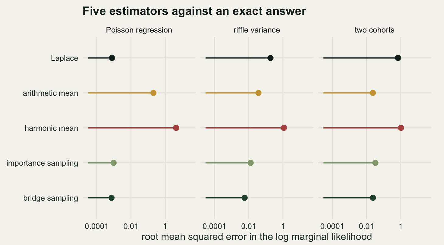
Reading down the bridge sampling row, the error is 7.29e-04 on the Poisson regression, 0.0057 on the riffle variance and 0.0238 on the two cohorts. The Laplace row goes 7.74e-04, 0.1849, 0.6952: excellent, then 32 times worse than bridge sampling, then 29 times worse. The harmonic mean is the worst estimator on every target, by 199 times on the riffle variance alone.
Two results in that table went against what I set out to write. Setting the harmonic mean aside, the arithmetic mean is the poorest of the sampling estimators on the Poisson regression, at 0.204, and respectable on the other two, 0.0369 and 0.0236, better than the Laplace approximation on both. Drawing from the prior is not intrinsically hopeless; it is hopeless in proportion to how much smaller the posterior is than the prior, and on the two narrow targets here the priors were not wide enough to destroy it. And the gain of bridge sampling over plain importance sampling is modest when the proposal fits well: factors of 1.32, 2.25 and 1.38 across the three. The case for bridge sampling is not that it wins here. It is what happens when the proposal does not fit, measured two sections below.
The reported relative errors deserve their own line, because the whole method depends on being able to trust them. Bridge sampling reports 6.32e-04, 5.55e-03 and 2.38e-02 on the three targets, against measured root mean squared errors of 7.29e-04, 5.73e-03 and 2.38e-02. Three for three, to within the noise of twenty replicates. That is a well calibrated standard error, and the next paragraph is why it should not be trusted on its own.
Run the same estimator on the chain that never left one mode. It returns -75.4647 against an exact -74.7709, an error of -0.6938 against minus the logarithm of two at -0.6931: the failure the Laplace approximation made, for the same reason. All 10000 draws are on one side of zero, so the integral being estimated is over half the parameter space. The reported relative error for that run is 2.48e-04. The method says it has four decimal places and it is wrong in the first. Multimodality is the one Laplace failure bridge sampling does not repair, because it repairs nothing about the sample it is handed: it inherits whatever the sampler found, and a standard error computed from those draws cannot see a region they never visited.
What the log scale hides: a Bayes factor
A marginal likelihood is quoted on the log scale, and log units flatten differences that matter. The riffle question makes that concrete. Fit the same dry masses without a riffle effect, integrate exactly, and take the ratio.
quad_pool <- function(hi, ng) {
  ge <- seq(1e-8, hi * pri_se, length.out = ng)
  lv <- vapply(ge, function(se) {
    a_s <- n_kick / se^2; b_s <- n_kick * gbar / se^2
    ldet <- n_kick * log(se^2) + log1p(tau_mu^2 * a_s)
    qf <- sum(lmass^2) / se^2 - tau_mu^2 * b_s^2 / (1 + tau_mu^2 * a_s)
    -0.5 * (n_kick * log(2 * pi) + ldet + qf) +
      dnorm(se, 0, pri_se, log = TRUE) + log(2)
  }, numeric(1))
  logsumexp(lv + log(replace(rep(1, ng), c(1, ng), 0.5))) + log(diff(ge)[1])
}
exact_pool <- quad_pool(8, 40001)
bf_of <- function(lm_site) exp(exact_pool - lm_site)
est_of <- function(nm) cmp$estimate[cmp$target == "riffle variance" &
                                      cmp$estimator == nm]
print(round(c(pooled_log_ml = exact_pool, riffle_log_ml = exact2,
              log_bf_for_pooling = exact_pool - exact2,
              bf_for_pooling = bf_of(exact2)), 4))
pooled_log_ml riffle_log_ml log_bf_for_pooling bf_for_pooling
-39.1039 -40.3006 1.1967 3.3092 print(round(c(bf_from_bridge = bf_of(est_of("bridge sampling")),
bf_from_laplace_log_scale = bf_of(lap2$logml),
bf_from_laplace_constrained = bf_of(lap2_con),
bf_from_harmonic_mean = bf_of(est_of("harmonic mean"))), 4)) bf_from_bridge bf_from_laplace_log_scale
3.3086 3.9814
bf_from_laplace_constrained bf_from_harmonic_mean
1.4608 1.2918 The pooled model has a log marginal likelihood of -39.1039 against -40.3006 for the model with a riffle effect, so the data favour pooling by a factor of 3.31. That is the kind of number a methods section reports and a reader acts on. Bridge sampling returns 3.31 for it. The Laplace approximation on the constrained scale, whose log error was only 0.818, returns 1.46, and the harmonic mean returns 1.29. An error of under one log unit is a different sentence in the paper: 3.3 to one for pooling is a decision, 1.5 to one is a shrug. An error the size the harmonic mean makes on the Poisson regression, 4.3 log units, is a factor of 75.
Both marginal likelihoods in a Bayes factor are usually estimated, so their errors compound. Here the pooled model is integrated exactly, which flatters every estimator by removing half the noise.
The requirements nobody writes down
Three things have to be true before any of this works, and none of them is usually stated next to the identity.
The first is that you need the unnormalised posterior at every draw, both the posterior draws and the proposal draws. That is the log likelihood plus the log prior, including every constant, and if the sampler dropped a constant for speed then every marginal likelihood built on it is out by that constant. Dropping the same constant in two models being compared cancels only if it really is the same constant.
The second is that the parameters have to be on an unbounded scale, with the Jacobian included. The proposal is a normal, and a normal puts mass outside the support of a bounded parameter, so a positive standard deviation goes to its logarithm and a probability goes to its logit. Changing variables changes the density, and the correction is the Jacobian term. Leaving it out does not produce an error message. It produces a different integral.
jac_tab <- t(vapply(c(1250, 2500, 5000), function(nn) {
  pd <- post2[seq_len(2 * nn), , drop = FALSE]
  bad <- both_est(lup2_nojac, pd, 7201)
  c(draws = nn, without_jacobian = bad$bridge,
    with_jacobian = both_est(lup2, pd, 7201)$bridge,
    reported_re = bad$re, error = bad$bridge - exact2)
}, numeric(5)))
print(round(jac_tab, 5))
draws without_jacobian with_jacobian reported_re error
[1,] 1250 -37.10168 -40.30772 0.01439 3.19891
[2,] 2500 -37.10045 -40.30213 0.01017 3.20014
[3,] 5000 -37.09169 -40.30119 0.00732 3.20890lapj <- laplace_at(lup2_nojac, c(log(0.2), log(0.5)))
chj <- rwm(lup2_nojac, lapj$mode, 44000, lapj$V * 2.4^2 / 2, 7300)
postj <- thin_of(chj, 4000, 4)
onej <- both_est(lup2_nojac, postj, 7301)
print(round(c(smallest_log_su_correct = min(post2[, 1]),
smallest_log_su_bugged = min(postj[, 1]),
bugged_bridge = onej$bridge, bugged_error = onej$bridge - exact2,
bugged_reported_re = onej$re), 4))smallest_log_su_correct smallest_log_su_bugged bugged_bridge
-9.7346 -22336.1203 -26.4570
bugged_error bugged_reported_re
13.8436 0.0256 With correct posterior draws and a bridge target missing the two Jacobian terms, the estimate is -37.092 against an exact -40.301, an error of 3.209 log units and a Bayes factor out by a factor of 25. Nothing about the run looks unwell. Across a fourfold range of sample size the wrong answer moves by 0.0100 log units, so it looks converged, and the reported relative error at the largest sample is 0.00732, so it looks precise. It is stable, precise and wrong.
The second block is the version that also reaches the sampler, which is the realistic case: one function is written for the log density on the transformed scale, the Jacobian is forgotten in it, and that function is passed both to the sampler and to the bridge routine. Without the Jacobian the density on the log scale does not vanish as the standard deviation goes to zero, so the target is improper and the chain walks off. Its smallest visited value of the log between-riffle standard deviation is -22336, against -9.73 for the correct chain; the estimate is -26.46 and the reported relative error is 0.0256. The diagnostic that catches this is in the draws, not in the estimator: a parameter that has wandered to minus twenty thousand on the log scale is visible in one call to range.
The third requirement is overlap between the proposal and the posterior. This is where bridge sampling earns the extra fifteen lines, so it is worth measuring rather than asserting. The proposal covariance is multiplied by a range of factors, and separately the proposal centre is moved away from the posterior in units of posterior standard deviation, with five replicate runs at each setting.
n_ov <- 5
ov_row <- function(fv, sv, seed0) {
  rr <- t(vapply(seq_len(n_ov), function(r)
    unlist(both_est(lup1, rep1[[r]], seed0 + r, infl = fv,
                    shift = sv)[c("is", "bridge", "ess", "re", "iter")]),
    numeric(5)))
  c(inflation = fv, shift = sv,
    is_rmse = sqrt(mean((rr[, "is"] - exact1)^2)),
    bridge_rmse = sqrt(mean((rr[, "bridge"] - exact1)^2)),
    weight_ess = mean(rr[, "ess"]), reported_re = mean(rr[, "re"]),
    iterations = max(rr[, "iter"]))
}
infl_grid <- c(0.02, 0.06, 0.2, 0.5, 1, 2, 8, 40, 150)
ovl <- as.data.frame(t(vapply(infl_grid, ov_row, numeric(7), sv = 0,
                              seed0 = 7400)))
shift_grid <- c(0, 1, 2, 3, 4, 6)
shf <- as.data.frame(t(vapply(shift_grid, function(sv) ov_row(1, sv, 7500),
                              numeric(7))))
print(round(ovl, 5))
inflation shift is_rmse bridge_rmse weight_ess reported_re iterations
1 0.02 0 1.43037 0.04078 21.86698 0.04650 9
2 0.06 0 0.57410 0.02683 29.68091 0.02844 8
3 0.20 0 0.07315 0.01171 96.27366 0.01490 7
4 0.50 0 0.02096 0.00382 1570.50479 0.00650 6
5 1.00 0 0.00076 0.00049 4978.15535 0.00065 5
6 2.00 0 0.01013 0.00736 3698.50194 0.00680 6
7 8.00 0 0.02111 0.02105 1155.87787 0.02007 7
8 40.00 0 0.05714 0.04306 246.83149 0.04291 9
9 150.00 0 0.17298 0.06992 68.27994 0.07475 10print(round(shf, 5)) inflation shift is_rmse bridge_rmse weight_ess reported_re iterations
1 1 0 0.00076 0.00071 4979.43923 0.00065 5
2 1 1 0.02113 0.01775 1377.57811 0.01178 7
3 1 2 0.06963 0.04587 126.58311 0.02726 8
4 1 3 0.47563 0.09433 25.47304 0.05531 9
5 1 4 1.75834 0.18136 10.27080 0.11955 11
6 1 6 8.57448 0.74059 4.05797 0.76987 200i_w <- which.max(ovl$is_rmse)
k_ov <- nrow(ovl); k_sh <- nrow(shf)
print(round(c(worst_inflation = ovl$inflation[i_w], worst_is = ovl$is_rmse[i_w],
bridge_there = ovl$bridge_rmse[i_w],
ratio = ovl$is_rmse[i_w] / ovl$bridge_rmse[i_w],
ess_there = ovl$weight_ess[i_w]), 4))worst_inflation worst_is bridge_there ratio ess_there
0.0200 1.4304 0.0408 35.0726 21.8670 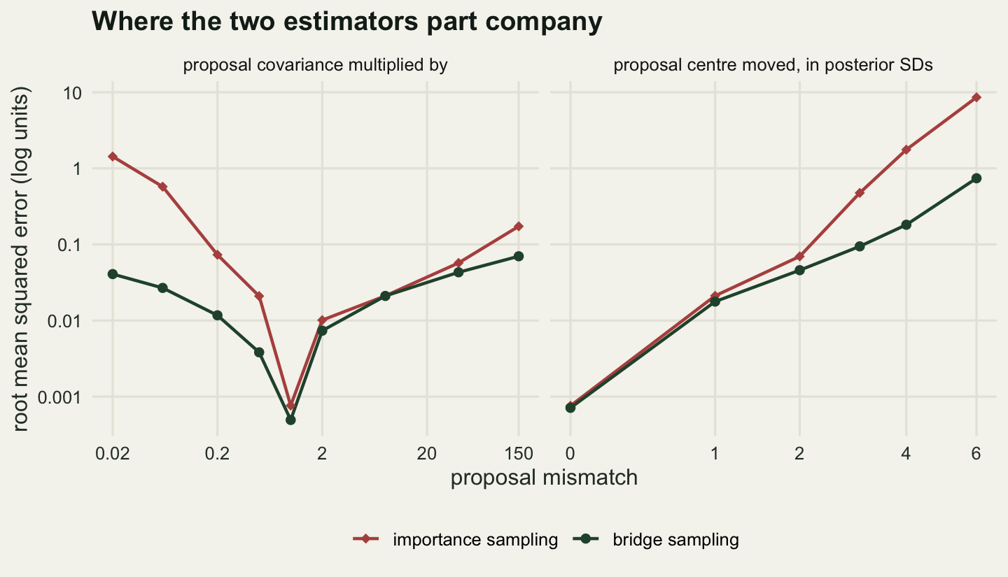
The asymmetry of the left panel is the point. A proposal that is too wide costs both methods errors of the same order: at 150 times the covariance, importance sampling is at 0.173 and bridge sampling at 0.070. A proposal that is too narrow is a different matter, because importance sampling then has no draws in the tails it needs and its weights degenerate. At 0.02 times the covariance, a proposal about 7 times too narrow in each direction, importance sampling is at 1.430 and bridge sampling at 0.041, a ratio of 35. The weight effective sample size there is 22 out of 5000, so the diagnostic did its job.
Moving the proposal off the posterior altogether breaks both. At a shift of 6 posterior standard deviations, importance sampling is out by 8.57 log units and bridge sampling by 0.74, which is better and still useless. Two things flag it: the reported relative error is 0.77, and the iteration failed to reach its tolerance in 200 steps, against 10 or fewer everywhere in the left panel.
How much of the answer is the prior
A posterior stops caring about a diffuse prior as data accumulate. A marginal likelihood never does, because the prior is what the likelihood is integrated against. The Poisson regression makes that measurable: vary the prior standard deviation on the sediment slope, hold everything else fixed, and compute the exact log Bayes factor against an intercept-only model at every setting. The intercept-only model is the same integral with the slope prior collapsed onto a point, so one grid function serves for both. Alongside it goes a WAIC difference between the same two models, computed from the grid weights so that no sampling noise enters.
waic_pois <- function(gr, yv, xv) {
  wt <- exp(gr$lp - max(gr$lp)); wt <- wt / sum(wt)
  lppd <- 0; pw <- 0
  for (i in seq_along(yv)) {
    eta <- outer(gr$g0, gr$g1 * xv[i], "+")
    lli <- yv[i] * eta - exp(eta) - lgamma(yv[i] + 1)
    mxx <- max(lli)
    lppd <- lppd + mxx + log(sum(wt * exp(lli - mxx)))
    mnv <- sum(wt * lli); pw <- pw + sum(wt * (lli - mnv)^2)
  }
  -2 * (lppd - pw)
}
null_of <- function(yv, xv) {
  c(logml = pois_grid(yv, xv, c(pri_sd[1], 1e-7), 1201)$logml,
    waic = waic_pois(pois_grid(yv, xv, c(pri_sd[1], 1e-7), 161), yv, xv))
}
sens_row <- function(tv, yv, xv, nullv, do_waic) {
  gr <- pois_grid(yv, xv, c(pri_sd[1], tv), 401)
  wt <- exp(gr$lp - max(gr$lp)); wt <- wt / sum(wt)
  mm <- sum(colSums(wt) * gr$g1)
  c(tau = tv, log_bf = gr$logml - nullv[["logml"]],
    delta_waic = if (do_waic)
      nullv[["waic"]] - waic_pois(pois_grid(yv, xv, c(pri_sd[1], tv), 161), yv, xv)
      else NA_real_,
    slope_mean = mm,
    slope_sd = sqrt(sum(colSums(wt) * gr$g1^2) - mm^2))
}
set.seed(20260809)
n_big <- 450
fines_b <- as.vector(scale(runif(n_big, 5, 60)))
y_big <- rpois(n_big, exp(1.75 - 0.55 * fines_b))
null1 <- null_of(y_kick, fines)
null_b <- null_of(y_big, fines_b)

tau_grid <- c(0.25, 0.5, 1, 2, 4, 8, 16, 32)
sens_s <- as.data.frame(t(vapply(tau_grid, sens_row, numeric(5), yv = y_kick,
                                 xv = fines, nullv = null1, do_waic = TRUE)))
sens_b <- as.data.frame(t(vapply(tau_grid, sens_row, numeric(5), yv = y_big,
                                 xv = fines_b, nullv = null_b, do_waic = FALSE)))
print(round(sens_s, 4))
tau log_bf delta_waic slope_mean slope_sd
1 0.25 32.8765 72.5423 -0.5070 0.0641
2 0.50 33.8315 72.7019 -0.5335 0.0663
3 1.00 33.5777 72.6862 -0.5407 0.0669
4 2.00 32.9963 72.6783 -0.5425 0.0671
5 4.00 32.3312 72.6760 -0.5430 0.0671
6 8.00 31.6451 72.6754 -0.5431 0.0671
7 16.00 30.9537 72.6753 -0.5431 0.0671
8 32.00 30.2610 72.6753 -0.5432 0.0671print(round(sens_b, 4)) tau log_bf delta_waic slope_mean slope_sd
1 0.25 370.1184 NA -0.5054 0.0191
2 0.50 370.9666 NA -0.5076 0.0191
3 1.00 370.6609 NA -0.5082 0.0192
4 2.00 370.0648 NA -0.5083 0.0192
5 4.00 369.3959 NA -0.5083 0.0192
6 8.00 368.7088 NA -0.5083 0.0192
7 16.00 368.0172 NA -0.5083 0.0192
8 32.00 367.3244 NA -0.5083 0.0192print(round(c(bf_range_45 = diff(range(sens_s$log_bf)),
bf_range_450 = diff(range(sens_b$log_bf)),
waic_range_45 = diff(range(sens_s$delta_waic)),
slope_range_45 = diff(range(sens_s$slope_mean)),
slope_range_450 = diff(range(sens_b$slope_mean)),
drop_per_doubling_45 = sens_s$log_bf[7] - sens_s$log_bf[8],
drop_per_doubling_450 = sens_b$log_bf[7] - sens_b$log_bf[8],
log_two = log(2)), 4)) bf_range_45 bf_range_450 waic_range_45
3.5705 3.6422 0.1596
slope_range_45 slope_range_450 drop_per_doubling_45
0.0362 0.0030 0.6927
drop_per_doubling_450 log_two
0.6928 0.6931 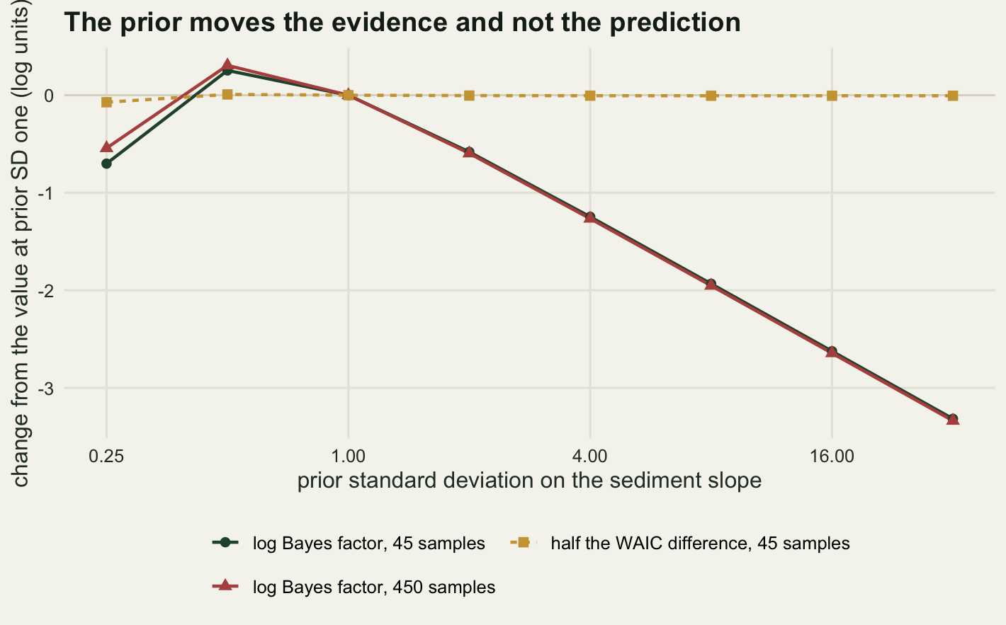
Over prior standard deviations from 0.25 to 32, none of which anyone would call unreasonable for a coefficient on a standardised covariate, the log Bayes factor moves by 3.571, a factor of 36. The posterior mean of the slope over the same range moves by 0.0362, from -0.543 to -0.507, and the WAIC difference moves by 0.160 on the deviance scale, 0.080 in log units. The predictive comparison does not notice the prior. The evidence comparison is made of it.
Ten times the data does not help. At 450 samples the posterior mean of the slope moves by 0.0030 across the same prior range, 12 times less than at 45, exactly as asymptotics promise. The log Bayes factor moves by 3.642, which is not less than the 3.571 at the smaller sample size. In the diffuse limit the arithmetic is clean: each doubling of the prior standard deviation costs the larger model 0.6927 at 45 samples and 0.6928 at 450, against a logarithm of two of 0.6931. That is the Ockham factor charging one halving of prior mass per doubling of prior width, and it does not care how much data there is.
Pushed to the limit this is the Lindley paradox (Lindley 1957): with a prior made diffuse enough, the Bayes factor favours the smaller model however strongly the data contradict it, so a diffuse prior is not a neutral choice but a strong vote for parsimony. Kass and Raftery (1995) give the standard treatment and the standard advice, which is to report the Bayes factor over a range of defensible priors rather than at one. A marginal likelihood with no prior sensitivity analysis beside it is half a result.
The honest limit
Every number here rests on a target small enough to integrate exactly, which is precisely the situation in which nobody needs bridge sampling. A real hierarchical model has no quadrature answer to check against, and then three of the supports used above disappear at once. There is no exact value, so the error cannot be measured, only estimated. The estimate rests entirely on the posterior sample it was built from, and the relative error the scheme reports is conditional on that sample being a good one, a condition it cannot check: on the chain that never left one mode it reported 2.48e-04 while sitting -0.694 from the truth. And a normal proposal fitted to the draws, which worked here in one and two dimensions, is a weaker approximation in twenty or two hundred, so the overlap the left panel of the mismatch figure measures gets worse with dimension in a way this post did not test.
The multimodality result is the one to carry away, because it is a limit of the method rather than of the demonstration. Bridge sampling estimates the integral of the unnormalised posterior over the region the draws explored. If half the posterior was never visited, the answer is the integral over the other half, and no number of extra bridge iterations, proposal draws or relative-error checks will say so. The remedies sit outside the estimator: a sampler that can cross, several chains started far apart, or knowing from the model’s structure that a symmetry exists, as it does whenever mixture components are unlabelled.
There is a wider limit that no computation reaches. A Bayes factor compares two models on the assumption that one of the pair generated the data. The riffle comparison asks whether the between-riffle standard deviation is exactly zero or drawn from a half-normal with scale 0.5, and the true answer is neither. Predictive scores make a weaker assumption and answer a weaker question, which is a reason to decide which one the ecology needs before reaching for either.
Where to go next
The natural next step is a model where no exact answer exists and the check has to come from somewhere else: run bridge sampling twice from independent chains and compare, or run it against a stepping-stone or thermodynamic-integration estimate, which pay much more computation for an estimator with a different failure mode. Vehtari, Gelman and Gabry (2017) is the reference for the predictive alternative, and running both on the same candidates is a cheap way to find out whether a conclusion depends on which question was asked.
References
Meng XL, Wong WH 1996 Statistica Sinica 6(4):831-860
Gelman A, Meng XL 1998 Statistical Science 13(2):163-185 (10.1214/ss/1028905934)
Gronau QF, Sarafoglou A, Matzke D, Ly A, Boehm U, Marsman M, Leslie DS, Forster JJ, Wagenmakers EJ, Steingroever H 2017 Journal of Mathematical Psychology 81:80-97 (10.1016/j.jmp.2017.09.005)
Newton MA, Raftery AE 1994 Journal of the Royal Statistical Society Series B 56(1):3-26 (10.1111/j.2517-6161.1994.tb01956.x)
Gelfand AE, Dey DK 1994 Journal of the Royal Statistical Society Series B 56(3):501-514 (10.1111/j.2517-6161.1994.tb01996.x)
Fruehwirth-Schnatter S 2004 Econometrics Journal 7(1):143-167 (10.1111/j.1368-423X.2004.00125.x)
Kass RE, Raftery AE 1995 Journal of the American Statistical Association 90(430):773-795 (10.1080/01621459.1995.10476572)
Lindley DV 1957 Biometrika 44(1-2):187-192 (10.1093/biomet/44.1-2.187)
Vehtari A, Gelman A, Gabry J 2017 Statistics and Computing 27(5):1413-1432 (10.1007/s11222-016-9696-4)