Checking a Bayesian computation

Four measured checks on an MCMC run in R: an exact benchmark, simulation-based calibration, divergences with the energy diagnostic, and Monte Carlo error.

The newt survey ran for six weeks and produced a spreadsheet with one row per pond visit and a zero or a one in the detection column. Twelve visits to the pond behind the sawmill, three detections. The question the project actually cares about is occupancy, but the number that has to come first is the detection probability, because everything downstream is conditional on it.

The detection probability came out of a sampler somebody in the group had written by hand. Not because a package would not have done it, but because the real model has a covariate on detection and a site-level random effect and a seasonal term, and by the time you have added those you are writing the log posterior yourself anyway. The sampler ran four chains overnight. R-hat came back at three digits of one. The effective sample sizes were in the tens of thousands. The traceplots were the fuzzy caterpillars everyone is taught to look for.

The posterior mean it reported was wrong by more than thirty Monte Carlo standard errors.

That is the situation this post is about. Not whether the model fits the data: a posterior predictive check answers that, and none of what follows does. The question here is narrower and comes first. Given the model you wrote down, did the sampler give you back the posterior distribution that model implies, or did it give you back some other distribution that happens to look stationary? Four checks answer that question, and each one catches something the others miss.

This post deliberately does not repeat MCMC convergence diagnostics from scratch, which builds R-hat and effective sample size by hand on a bimodal target and shows a single chain that looks converged and is not. Those two statistics are reused here without being rebuilt, and their limitation is exactly the point: they measure whether the chains agree with each other and how much information the draws carry, and a sampler that is stationary at the wrong distribution passes both. The four checks below are the ones that post does not cover. The Hamiltonian machinery comes from Hamiltonian Monte Carlo from scratch, the funnel geometry from reparameterisation and Neal’s funnel, and the closed-form comparison target from the Laplace approximation in R.

Everything is base R plus ggplot2. The samplers are a Metropolis loop and a leapfrog integrator, both written out in full, and the whole post knits in well under a minute.

library(ggplot2)

te_pal <- list(forest = "#275139", green = "#2f8f63", sage = "#93a87f",
               clay = "#b5534e", gold = "#cda23f", line = "#dad9ca",
               ink = "#16241d", paper = "#f5f4ee")

int <- function(x) formatC(x, format = "d", big.mark = "")
fmt <- function(x, digits = 4) formatC(x, format = "f", digits = digits)

theme_te <- function() {
  theme_minimal(base_size = 12) +
    theme(panel.grid.minor = element_blank(),
          panel.grid.major = element_line(colour = "#e7e6dc"),
          plot.background = element_rect(fill = "#f5f4ee", colour = NA),
          panel.background = element_rect(fill = "#f5f4ee", colour = NA),
          plot.title = element_text(face = "bold", colour = te_pal$ink),
          axis.title = element_text(colour = "#2c3a31"),
          legend.position = "bottom")
}

The two statistics that are not going to save you

Both checks in this section are borrowed, not built. Split R-hat compares the variance between chain halves with the variance within them, and effective sample size divides the number of draws by the integrated autocorrelation time, estimated here with Geyer’s initial monotone sequence. Twenty lines of base R each.

rhat_split <- function(sims) {
  n <- nrow(sims); h <- floor(n / 2)
  s <- cbind(sims[1:h, , drop = FALSE], sims[(n - h + 1):n, , drop = FALSE])
  nn <- nrow(s); cm <- colMeans(s); cv <- apply(s, 2, var)
  vhat <- ((nn - 1) * mean(cv) + nn * var(cm)) / nn
  sqrt(vhat / mean(cv))
}

ess_geyer <- function(sims) {
  n <- nrow(sims); m <- ncol(sims); lag_max <- min(n - 1, 400)
  ac <- sapply(seq_len(m), function(j)
    acf(sims[, j], lag.max = lag_max, plot = FALSE)$acf[, 1, 1])
  rho <- rowMeans(matrix(ac, ncol = m))
  kmax <- floor((length(rho) - 1) / 2)
  gam <- rho[2 * (1:kmax)] + rho[2 * (1:kmax) + 1]
  neg <- which(gam <= 0); kk <- if (length(neg)) neg[1] - 1 else kmax
  if (kk < 1) return(m * n)
  m * n / max(-1 + 2 * sum(cummin(gam[1:kk])), 1)
}

Neither function looks at the model. rhat_split sees a matrix of numbers and asks whether the columns agree; ess_geyer sees the same matrix and asks how fast the correlation decays. If four chains all wander happily around a distribution that is not your posterior, they agree with each other perfectly and the autocorrelation decays exactly as it should. Both statistics come back clean. That is not a flaw in them, it is what they were designed to measure, and it is the reason the rest of this post exists.

A model whose answer is already known

The benchmark model is the smallest useful one in the detection literature: 3 detections in 12 visits, with a uniform prior on the detection probability. The posterior is a beta distribution and every quantile of it is available from qbeta to machine precision.

n_visit <- 12; y_det <- 3; a_pri <- 1; b_pri <- 1
post_a <- a_pri + y_det; post_b <- b_pri + n_visit - y_det
post_sd <- sqrt(post_a * post_b /
                ((post_a + post_b)^2 * (post_a + post_b + 1)))
print(round(c(visits = n_visit, detections = y_det,
              prior_a = a_pri, prior_b = b_pri,
              post_a = post_a, post_b = post_b,
              post_mean = post_a / (post_a + post_b),
              post_sd = post_sd), 5))

    visits detections    prior_a    prior_b     post_a     post_b  post_mean 
  12.00000    3.00000    1.00000    1.00000    4.00000   10.00000    0.28571 
   post_sd 
   0.11664 

So the target is a Beta(4, 10) with mean 0.28571 and standard deviation 0.11664. Now write a sampler for it the way you would write a sampler for the real model. A probability lives in the unit interval and a random walk proposal does not respect that, so you move to the log odds scale \(z = \log(\theta / (1 - \theta))\) and propose there. That change of variable is where the trouble starts, because a density does not transform like a function. It picks up the absolute derivative of the inverse map, and for the logistic that factor is \(\theta(1 - \theta)\), which on the log scale is the sum of the two log-probabilities.

logpost_z <- function(z, y, n, jac = TRUE) {
  lt <- plogis(z, log.p = TRUE); lu <- plogis(-z, log.p = TRUE)
  out <- (y + a_pri - 1) * lt + (n - y + b_pri - 1) * lu
  if (jac) out + lt + lu else out
}

run_rw <- function(n_iter, step, z0, jac, y = y_det, n = n_visit) {
  keep <- numeric(n_iter); cur <- z0
  lcur <- logpost_z(cur, y, n, jac); n_acc <- 0
  for (i in seq_len(n_iter)) {
    prop <- cur + rnorm(1, 0, step)
    lp <- logpost_z(prop, y, n, jac)
    if (log(runif(1)) < lp - lcur) { cur <- prop; lcur <- lp; n_acc <- n_acc + 1 }
    keep[i] <- cur
  }
  list(z = keep, acc = n_acc / n_iter)
}

The jac argument is the deliberate bug. With jac = TRUE the two extra log terms are the log Jacobian and the sampler targets the true posterior. With jac = FALSE they are missing, which is the single most common error in hand-written ecological samplers: you transform a bounded parameter to make the proposal easier, and you forget that the prior density has to be transformed too. Nothing in the code errors. Nothing in the output looks strange. The sampler simply targets a different distribution, in this case a Beta(3, 9), and it targets it beautifully.

set.seed(20260729)
n_chain <- 4; n_iter <- 12000; n_warm <- 2000; rw_step <- 1.2
inits <- c(-3, -1, 0, 1.5)

draw_theta <- function(jac) {
  M <- matrix(NA_real_, n_iter - n_warm, n_chain); a <- numeric(n_chain)
  for (j in seq_len(n_chain)) {
    r <- run_rw(n_iter, rw_step, inits[j], jac)
    M[, j] <- plogis(r$z[(n_warm + 1):n_iter]); a[j] <- r$acc
  }
  list(theta = M, acc = mean(a))
}

fit_ok <- draw_theta(TRUE)
fit_bad <- draw_theta(FALSE)
print(c(chains = n_chain, iter_per_chain = n_iter, warmup = n_warm,
        kept_draws = length(fit_ok$theta)))

        chains iter_per_chain         warmup     kept_draws 
             4          12000           2000          40000 

print(round(c(proposal_sd = rw_step, accept_correct = fit_ok$acc,
              accept_broken = fit_bad$acc), 4))

   proposal_sd accept_correct  accept_broken 
        1.2000         0.5072         0.5421 

Four chains of 12000 iterations with the first 2000 discarded gives 40000 draws per sampler. Acceptance is 0.5072 for the correct target and 0.5421 for the broken one, both in the range a tuning routine would aim for on a one-dimensional random walk. Nothing to report so far.

Check one: the exact benchmark

Run the standard diagnostics on both samplers first, so that the rest of the section has something to argue against.

diag_row <- function(M, lab) {
  e <- ess_geyer(M)
  data.frame(sampler = lab, rhat = round(rhat_split(M), 4), ess = round(e),
             post_mean = round(mean(M), 5),
             mcse = round(sd(as.vector(M)) / sqrt(e), 5))
}
conv <- rbind(diag_row(fit_ok$theta, "correct"),
              diag_row(fit_bad$theta, "no Jacobian"))
conv$exact <- round(post_a / (post_a + post_b), 5)
conv$z <- round((conv$post_mean - conv$exact) / conv$mcse, 2)
print(conv)

      sampler   rhat   ess post_mean    mcse   exact      z
1     correct 1.0001 16210   0.28623 0.00092 0.28571   0.57
2 no Jacobian 1.0003 13280   0.25203 0.00104 0.28571 -32.38

print(round(c(broken_target_mean = (post_a - 1) / (post_a + post_b - 2)), 5))

broken_target_mean 
              0.25 

The broken sampler has an R-hat of 1.0003 and an effective sample size of 13280. Those are not marginal passes. They are the numbers you would put in a supplement to demonstrate that the computation was sound. The correct sampler has R-hat 1.0001 and effective sample size 16210, and the two are indistinguishable on any convergence criterion anyone uses.

The last column is the benchmark. Take the difference between the sampled posterior mean and the exact posterior mean, and divide it by the Monte Carlo standard error of the sampled mean, which is the posterior standard deviation divided by the square root of the effective sample size. For the correct sampler that ratio is 0.57, comfortably inside the noise. For the broken sampler it is -32.38. The reported mean is 0.25203 against a true 0.28571, and the broken sampler’s own target, Beta(3, 9), has mean exactly 0.25. The sampler did its job perfectly. The job was the wrong one.

The mean is only one summary, and a sampler can get the mean right and the spread wrong, so run the comparison across the quantiles as well. The Monte Carlo standard error of a sampled quantile is not the same formula as for a mean. It is \(\sqrt{p(1-p)/S_p}\) divided by the posterior density at that quantile, where \(S_p\) is the effective sample size of the indicator series that flags draws below the quantile. The density is taken from a kernel estimate on the draws themselves, so the whole thing stays self-contained.

q_lev <- c(0.025, 0.25, 0.5, 0.75, 0.975)
q_exact <- qbeta(q_lev, post_a, post_b)

bench <- function(M, lab) {
  x <- as.vector(M)
  qh <- quantile(x, q_lev, names = FALSE)
  dd <- density(x, n = 2048, from = 0, to = 1)
  fq <- approx(dd$x, dd$y, xout = qh)$y
  se <- numeric(length(q_lev))
  for (k in seq_along(q_lev)) {
    e <- ess_geyer((M <= qh[k]) * 1)
    se[k] <- sqrt(q_lev[k] * (1 - q_lev[k]) / e) / fq[k]
  }
  data.frame(sampler = lab, level = q_lev, exact = round(q_exact, 5),
             sampled = round(qh, 5), mcse = round(se, 5),
             z = round((qh - q_exact) / se, 2))
}

bench_tab <- rbind(bench(fit_ok$theta, "correct"),
                   bench(fit_bad$theta, "no Jacobian"))
print(bench_tab)

       sampler level   exact sampled    mcse      z
1      correct 0.025 0.09092 0.09290 0.00126   1.58
2      correct 0.250 0.19913 0.19958 0.00101   0.45
3      correct 0.500 0.27528 0.27558 0.00102   0.30
4      correct 0.750 0.36148 0.35992 0.00126  -1.24
5      correct 0.975 0.53813 0.54003 0.00221   0.86
6  no Jacobian 0.025 0.09092 0.06313 0.00117 -23.79
7  no Jacobian 0.250 0.19913 0.16343 0.00105 -34.10
8  no Jacobian 0.500 0.27528 0.23748 0.00110 -34.49
9  no Jacobian 0.750 0.36148 0.32650 0.00135 -25.99
10 no Jacobian 0.975 0.53813 0.51826 0.00268  -7.42

print(round(c(max_abs_z_correct = max(abs(bench_tab$z[1:5])),
              max_abs_z_broken = max(abs(bench_tab$z[6:10]))), 2))

max_abs_z_correct  max_abs_z_broken 
             1.58             34.49 

print(round(c(gap_at_lowest_level =
                bench_tab$sampled[1] - bench_tab$exact[1]), 5))

gap_at_lowest_level 
            0.00198 

Every one of the five comparisons for the correct sampler lands inside two standard errors; the largest absolute value is 1.58. That is what a passing benchmark looks like, and the standard error is what makes it a pass rather than a shrug: without it you would be staring at a difference of 0.00198 at the 0.025 quantile and wondering whether that mattered.

For the broken sampler the largest absolute value is 34.49. The pattern across the five levels is worth reading rather than summarising. At the median the deviation is -34.49 standard errors and at the 0.975 quantile it is -7.42. The bug does not shift the posterior rigidly. It bites hardest in the body and least in the upper tail, which is exactly what you would expect from a missing \(\theta(1-\theta)\) factor: that factor is smallest where the probability is nearest zero or one.

bt <- bench_tab
bt$sampler <- factor(bt$sampler, levels = c("correct", "no Jacobian"))
ggplot(bt, aes(level, z, colour = sampler, shape = sampler)) +
  annotate("rect", xmin = 0, xmax = 1, ymin = -2, ymax = 2,
           fill = te_pal$sage, alpha = 0.35) +
  geom_hline(yintercept = 0, colour = te_pal$ink, linewidth = 0.4) +
  geom_line(linewidth = 0.7) +
  geom_point(size = 2.8) +
  annotate("text", x = 0.5, y = 5.5, label = "plus or minus 2 standard errors",
           colour = "#2c3a31", size = 3.2) +
  scale_colour_manual(values = c(correct = te_pal$green,
                                 `no Jacobian` = te_pal$clay)) +
  scale_shape_manual(values = c(correct = 16, `no Jacobian` = 17)) +
  scale_x_continuous(breaks = q_lev) +
  labs(x = "posterior quantile level",
       y = "(sampled - exact) / Monte Carlo SE",
       colour = NULL, shape = NULL,
       title = "Sampled quantiles against the exact beta posterior") +
  theme_te()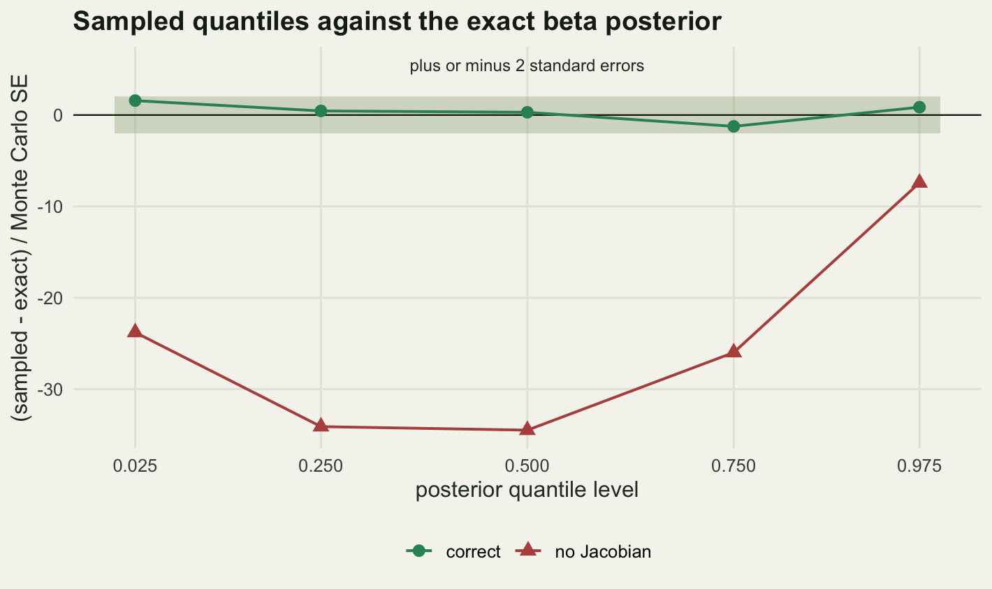

Figure 1: Sampled posterior quantiles minus the exact beta quantiles, expressed in Monte Carlo standard errors. The correct sampler (green circles) stays inside the shaded plus or minus two band at all five levels; the sampler with the missing Jacobian (red triangles) sits between -7.42 and -34.50.

The benchmark is the cheapest of the four checks and the one people skip most often, because it feels like a test of something you already know. It is not. It is a test of the code path, and the code path is shared: the same transformation helper, the same prior function, the same acceptance rule that will carry the real model. Running the real sampler on a conjugate special case, where you can delete the covariates and set the random effect variance to zero and read the answer off qbeta, costs a few minutes and catches the class of bug that no amount of chain-watching will.

Check two: simulation-based calibration

The benchmark works because the posterior is known. On the real model it is not, and the benchmark has nothing to compare against. Simulation-based calibration replaces the known posterior with a known joint distribution, which you always have, because you wrote the prior and the likelihood yourself.

The argument is short. Draw a parameter from the prior. Simulate a dataset from the likelihood at that parameter. Fit the model to that dataset and take posterior draws. Now count how many of those draws fall below the parameter that generated the data. If the sampler returns the correct posterior, that count is uniformly distributed over its possible values, and it is uniform for every prior draw, so it stays uniform when you pool across replicates. The reason is that the prior draw and the posterior draws are exchangeable given the data. With 15 posterior draws the rank can take 16 values, and 16 equally likely values is a clean chi-squared test with no binning choices to argue about.

sbc_narrow <- 0.6; sbc_wide <- 1.6; sbc_shift <- 0.4

rw_thin <- function(y, n_keep, warm, thin, jac) {
  cur <- 0; lcur <- logpost_z(cur, y, n_visit, jac)
  total <- warm + n_keep * thin; out <- numeric(n_keep); k <- 0
  for (i in seq_len(total)) {
    prop <- cur + rnorm(1, 0, rw_step)
    lp <- logpost_z(prop, y, n_visit, jac)
    if (log(runif(1)) < lp - lcur) { cur <- prop; lcur <- lp }
    if (i > warm && ((i - warm) %% thin == 0)) { k <- k + 1; out[k] <- cur }
  }
  plogis(out)
}

Thinning is not a stylistic choice here. The rank statistic assumes the posterior draws are independent, and an autocorrelated chain gives ranks that are too smooth, which shows up as a false hill in the middle of the histogram. Thinning by a factor well above the integrated autocorrelation time is the standard fix and the one used below.

Six samplers go through the same machinery. Two of them are correct: exact conjugate draws from rbeta, and the thinned Metropolis sampler with the Jacobian. One is the Jacobian bug from the previous section. The last three are deliberate distortions of the exact posterior on the log odds scale, so that the characteristic histogram shapes can be seen next to each other: a posterior squeezed to 0.6 of its width, one stretched to 1.6, and one shifted by 0.4 of a posterior standard deviation.

set.seed(20260730)
n_rep <- 400; n_draw <- 15; n_bin <- n_draw + 1
sbc_warm <- 250; sbc_thin <- 25
theta_true <- rbeta(n_rep, a_pri, b_pri)
y_sim <- rbinom(n_rep, n_visit, theta_true)
sbc_lab <- c("exact conjugate", "Metropolis, correct", "Metropolis, no Jacobian",
             "posterior too narrow", "posterior too wide", "posterior shifted")
ranks <- matrix(NA_integer_, n_rep, 6)

for (r in seq_len(n_rep)) {
  y <- y_sim[r]; tt <- theta_true[r]
  aa <- a_pri + y; bb <- b_pri + n_visit - y
  ex <- rbeta(n_draw, aa, bb); zz <- qlogis(ex)
  mz <- digamma(aa) - digamma(bb); sz <- sqrt(trigamma(aa) + trigamma(bb))
  ranks[r, 1] <- sum(ex < tt)
  ranks[r, 2] <- sum(rw_thin(y, n_draw, sbc_warm, sbc_thin, TRUE) < tt)
  ranks[r, 3] <- sum(rw_thin(y, n_draw, sbc_warm, sbc_thin, FALSE) < tt)
  ranks[r, 4] <- sum(plogis(mz + sbc_narrow * (zz - mz)) < tt)
  ranks[r, 5] <- sum(plogis(mz + sbc_wide * (zz - mz)) < tt)
  ranks[r, 6] <- sum(plogis(zz + sbc_shift * sz) < tt)
}
print(c(replicates = n_rep, draws_per_fit = n_draw, bins = n_bin,
        df = n_bin - 1, expected_per_bin = n_rep / n_bin,
        sbc_warmup = sbc_warm, sbc_thin = sbc_thin))

      replicates    draws_per_fit             bins               df 
             400               15               16               15 
expected_per_bin       sbc_warmup         sbc_thin 
              25              250               25 

print(round(c(narrow_factor = sbc_narrow, wide_factor = sbc_wide,
              shift_in_sd = sbc_shift, chisq_crit_level = 0.95,
              chisq_crit_value = qchisq(0.95, n_bin - 1)), 3))

   narrow_factor      wide_factor      shift_in_sd chisq_crit_level 
           0.600            1.600            0.400            0.950 
chisq_crit_value 
          24.996 

400 replicates, 15 posterior draws each, 16 rank values, 15 degrees of freedom, 25 runs expected in each bin. The 0.95 critical value of the chi-squared statistic is 24.996.

exp_bin <- n_rep / n_bin
sbc_tab <- data.frame(sampler = sbc_lab,
  chisq = round(apply(ranks, 2, function(x)
    sum((tabulate(x + 1, n_bin) - exp_bin)^2 / exp_bin)), 2))
sbc_tab$lowest_bin <- apply(ranks, 2, function(x) sum(x == 0))
sbc_tab$highest_bin <- apply(ranks, 2, function(x) sum(x == n_draw))
sbc_tab$middle_four <- apply(ranks, 2, function(x) sum(x >= 6 & x <= 9))
print(sbc_tab)

                  sampler  chisq lowest_bin highest_bin middle_four
1         exact conjugate  13.92         16          29         113
2     Metropolis, correct  15.36         23          18         109
3 Metropolis, no Jacobian  56.24         41          54          94
4    posterior too narrow 121.04         54          65          68
5      posterior too wide 113.04          4           7         167
6       posterior shifted  64.96         40          11         100

print(c(expected_per_bin = exp_bin, expected_middle_four = 4 * exp_bin))

    expected_per_bin expected_middle_four 
                  25                  100 

The two correct samplers give 13.92 and 15.36, both far below the critical value, and the fact that the thinned Metropolis sampler scores as flat as exact conjugate draws is the positive control this check needs. Everything else fails, and the failures are distinguishable by shape rather than by magnitude.

rk_df <- do.call(rbind, lapply(seq_len(6), function(j)
  data.frame(rank = 0:n_draw, count = tabulate(ranks[, j] + 1, n_bin),
             sampler = sbc_lab[j],
             verdict = if (j <= 2) "calibrated" else "not calibrated")))
rk_df$sampler <- factor(rk_df$sampler, levels = sbc_lab)

ggplot(rk_df, aes(rank, count, fill = verdict)) +
  geom_col(width = 0.85) +
  geom_hline(yintercept = exp_bin, colour = te_pal$ink,
             linetype = 2, linewidth = 0.4) +
  facet_wrap(~ sampler, ncol = 3) +
  scale_fill_manual(values = c(calibrated = te_pal$green,
                               `not calibrated` = te_pal$clay)) +
  labs(x = "rank of the true value among 15 posterior draws",
       y = "number of simulations", fill = NULL,
       title = "Rank histograms from 400 calibration runs") +
  theme_te()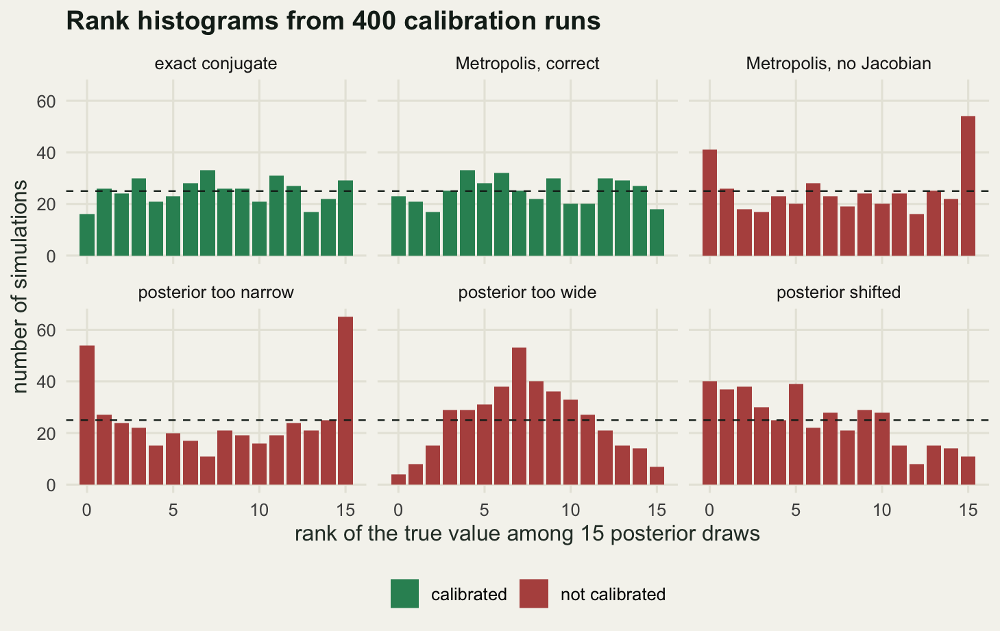

Figure 2: Rank of the true parameter among 15 posterior draws, pooled over 400 simulated datasets, for six samplers. The two calibrated samplers (green) scatter around the dashed line at 25. Among the four broken ones (red), the too-narrow posterior gives a deep U, the too-wide one gives a hill, the shifted one gives a downward slope, and the missing Jacobian gives a shallower U of its own, its right-hand spike the taller of the two.

The squeezed posterior scores 121.04, with 54 runs in the lowest bin and 65 in the highest against an expectation of 25 in each, and only 68 in the middle four bins where 100 are expected. That is the U. A posterior that is too narrow leaves the true value outside the draws too often, and outside means either above all of them or below all of them, so both ends fill up.

The stretched posterior scores 113.04 and does the opposite: 4 and 7 at the ends, 167 in the middle four. The true value keeps landing comfortably inside a posterior that is wider than it should be, so the ranks crowd the centre. The shifted posterior scores 64.96, with 40 runs at rank zero and only 11 at rank 15: a slope, because the draws sit above the truth more often than below it.

Now the result that does not follow the script. The Jacobian bug scores 56.24, well past the critical value, so simulation-based calibration catches it. But the shape it produces is a U: 41 runs at the lowest rank and 54 at the highest, while the middle four bins hold 94 against the 100 expected. The excess is concentrated at the two ends and the centre is untouched. Read off the usual crib sheet, that says the posterior is too narrow. It is not. The broken sampler’s target, Beta(3, 9), is very slightly wider than the true posterior. What the missing Jacobian actually does is push the posterior away from one half, upward when the detection rate is above one half and downward when it is below, and the direction flips with the data. Averaged over 400 prior draws that becomes a symmetric miscentring, and a symmetric miscentring puts the truth in the tails just as reliably as a narrow posterior does.

So the shape vocabulary names a symptom, not a cause. A U means the true value lands in the tails too often, which a squeezed posterior and a data-dependent shift both produce. That matters in practice, because a U-shaped rank histogram usually gets diagnosed as underdispersion and treated by widening priors or lengthening chains, and neither of those would have touched this bug. The exact benchmark, which said the mean was off by -32.38 standard errors and pointed at a specific target distribution, told you far more about where to look.

There is also a cost worth stating plainly. This whole check is 400 independent fits. Here that is 400 short Metropolis runs on a one-parameter model and it takes seconds. For a hierarchical occupancy model that needs ten minutes a fit, 400 fits is nearly three days of compute. That is the real reason almost nobody in ecology runs simulation-based calibration, and it is also why the honest version is to run it once, on a reduced version of the model, before the analysis rather than after.

Check three: divergences and the energy diagnostic

The first two checks apply to any sampler. This one is specific to gradient based samplers, and it exists because those samplers fail in a way that leaves a fingerprint. A leapfrog integrator that hits a region where the log posterior curves too sharply for the step size loses energy conservation catastrophically, and the numerical Hamiltonian shoots off. Flagging those transitions costs one comparison per step.

hmc <- function(logp, glogp, q0, n_it, eps, n_leap, delta_max = 1000) {
  d <- length(q0)
  out <- matrix(NA_real_, n_it, d); dv <- logical(n_it); en <- numeric(n_it)
  q <- q0; lp <- logp(q); n_acc <- 0
  for (i in seq_len(n_it)) {
    mom <- rnorm(d); h0 <- -lp + 0.5 * sum(mom^2); en[i] <- h0
    qq <- q; pp <- mom; lpp <- lp; gg <- glogp(qq); bad <- FALSE; hh <- h0
    for (l in seq_len(n_leap)) {
      pp <- pp + 0.5 * eps * gg
      qq <- qq + eps * pp
      gg <- glogp(qq)
      pp <- pp + 0.5 * eps * gg
      lpp <- logp(qq); hh <- -lpp + 0.5 * sum(pp^2)
      if (!is.finite(hh) || (hh - h0) > delta_max) { bad <- TRUE; break }
    }
    if (!bad && log(runif(1)) < h0 - hh) { q <- qq; lp <- lpp; n_acc <- n_acc + 1 }
    out[i, ] <- q; dv[i] <- bad
  }
  list(draws = out, div = dv, energy = en, acc = n_acc / n_it)
}

The en vector is the second diagnostic. It stores the Hamiltonian right after the momentum is redrawn, once per iteration. The energy fraction of missing information compares the variance of the change in that quantity between consecutive iterations with its marginal variance. If a single momentum refresh typically moves the energy about as far as the energy varies overall, the sampler can traverse the whole distribution and the ratio sits near one. If the energy has heavy tails that the momentum refresh cannot reach in one step, the ratio collapses, and it collapses for geometric reasons that leave the autocorrelation within each chain looking perfectly ordinary.

The target is the funnel: a log scale parameter and 9 latent values whose spread is governed by it, which is the shape every hierarchical model with a weakly identified variance component takes on.

n_x <- 9
lp_cen <- function(q) {
  v <- q[1]; x <- q[-1]
  -v^2 / 18 - n_x * v / 2 - 0.5 * exp(-v) * sum(x^2)
}
gl_cen <- function(q) {
  v <- q[1]; x <- q[-1]
  c(-v / 9 - n_x / 2 + 0.5 * exp(-v) * sum(x^2), -exp(-v) * x)
}
lp_nc <- function(q) -0.5 * sum(q^2)
gl_nc <- function(q) -q

The centred version samples the latent values directly, so their scale depends on where the log scale parameter currently is. The non-centred version samples standardised values and multiplies afterwards, which leaves a spherical Gaussian target and recovers the same distribution. Both are run at the same settings, and the centred one is also run at a smaller and a larger step size, because the step size turns out to matter more than expected.

hmc_iter <- 2500; hmc_warm <- 500; n_leap <- 20

run_hmc <- function(lp, gl, centred, eps) {
  kp <- (hmc_warm + 1):hmc_iter; nk <- length(kp)
  V <- matrix(NA_real_, nk, n_chain); X <- V; E <- V
  D <- matrix(NA, nk, n_chain); a <- numeric(n_chain)
  for (j in seq_len(n_chain)) {
    r <- hmc(lp, gl, rnorm(n_x + 1) * 0.5, hmc_iter, eps, n_leap)
    d <- r$draws[kp, ]
    if (centred) { V[, j] <- d[, 1]; X[, j] <- d[, 2] }
    else { V[, j] <- 3 * d[, 1]; X[, j] <- exp(3 * d[, 1] / 2) * d[, 2] }
    D[, j] <- r$div[kp]; E[, j] <- r$energy[kp]; a[j] <- r$acc
  }
  list(V = V, X = X, D = D, acc = mean(a), div_rate = mean(D), n_div = sum(D),
       ebfmi = mean(apply(E, 2, function(e)
         sum(diff(e)^2) / (length(e) * var(e)))),
       rhat = rhat_split(V), ess = ess_geyer(V),
       mean_v = mean(V), sd_v = sd(as.vector(V)),
       q05 = quantile(as.vector(V), 0.05, names = FALSE))
}

set.seed(20260731)
hmc_runs <- list(run_hmc(lp_cen, gl_cen, TRUE, 0.2),
                 run_hmc(lp_cen, gl_cen, TRUE, 0.4),
                 run_hmc(lp_cen, gl_cen, TRUE, 0.6),
                 run_hmc(lp_nc, gl_nc, FALSE, 0.4))
hmc_tab <- data.frame(
  run = c("centred, step 0.2", "centred, step 0.4", "centred, step 0.6",
          "non-centred, step 0.4"),
  accept = round(sapply(hmc_runs, function(o) o$acc), 4),
  div_rate = round(sapply(hmc_runs, function(o) o$div_rate), 4),
  n_div = sapply(hmc_runs, function(o) o$n_div),
  ebfmi = round(sapply(hmc_runs, function(o) o$ebfmi), 4),
  rhat = round(sapply(hmc_runs, function(o) o$rhat), 4),
  ess = round(sapply(hmc_runs, function(o) o$ess)),
  sd_v = round(sapply(hmc_runs, function(o) o$sd_v), 4),
  q05_v = round(sapply(hmc_runs, function(o) o$q05), 4))
print(hmc_tab)

                    run accept div_rate n_div  ebfmi   rhat  ess   sd_v   q05_v
1     centred, step 0.2 0.9264   0.0000     0 0.0840 1.0326   91 2.3908 -3.5778
2     centred, step 0.4 0.6971   0.0144   115 0.0964 1.0631   90 2.3040 -2.7762
3     centred, step 0.6 0.3588   0.1895  1516 0.1052 1.1195   51 2.1677 -2.1899
4 non-centred, step 0.4 0.9514   0.0000     0 1.0401 0.9999 8000 2.9430 -4.8929

print(c(hmc_chains = n_chain, hmc_iter = hmc_iter, hmc_warmup = hmc_warm,
        leapfrog = n_leap, latent_x = n_x, kept = length(hmc_runs[[1]]$V)))

hmc_chains   hmc_iter hmc_warmup   leapfrog   latent_x       kept 
         4       2500        500         20          9       8000 

print(round(c(true_sd_v = 3, true_q05_v = qnorm(0.05, 0, 3),
              rhat_rule_old = 1.1, rhat_rule_modern = 1.01,
              ebfmi_warning_line = 0.3), 4))

         true_sd_v         true_q05_v      rhat_rule_old   rhat_rule_modern 
            3.0000            -4.9346             1.1000             1.0100 
ebfmi_warning_line 
            0.3000 

Start with the two runs at step 0.4. The non-centred one is a clean sheet: divergence rate 0.0000, energy fraction 1.0401, R-hat 0.9999, an effective sample size of 8000 from 8000 draws (the estimator floors the autocorrelation time at one, so the whole sample counts), and a recovered standard deviation of 2.9430 against a true 3. The centred one at the same step size has 115 divergent transitions, an energy fraction of 0.0964, and a recovered standard deviation of 2.3040. The fifth percentile of the log scale parameter comes back as -2.7762 when the truth is -4.9346. The sampler simply never visits the narrow part of the funnel, and in a real hierarchical model that region is where the random effect variance is near zero, which is often the hypothesis the paper is testing.

R-hat for that run is 1.0631. Under the threshold of 1.1 that most ecological papers still cite, that is a pass. It fails the modern threshold of 1.01, which is a good part of the argument for the modern threshold, but the value is still small enough that most people would answer it by running longer chains rather than by suspecting the geometry.

Now the part that goes against the obvious reading. Compare the three centred runs. At step 0.6 the divergence rate is 0.1895, which nobody could miss. At step 0.4 it is 0.0144. At step 0.2 it is 0.0000, that is 0 divergent transitions in 8000 draws, which any automatic check would report as effectively zero. And the answer is still wrong: the recovered standard deviation at the small step is 2.3908 against a true 3, and the fifth percentile is -3.5778 against -4.9346.

Shrinking the step size does not fix the geometry. It makes the integrator accurate enough to stop failing loudly, while leaving it far too slow to actually cross the neck of the funnel within the trajectory length it is given. The bias survives and the alarm goes quiet. Meanwhile the energy fraction is 0.0840 at the small step, 0.0964 in the middle and 0.1052 at the large step: all three sit far below the conventional warning line of 0.3, and all three are an order of magnitude below the 1.0401 the non-centred run achieves. The energy diagnostic is the one that stays honest across the whole step size range, and it is the one almost nobody looks at.

cc <- hmc_runs[[2]]; nc <- hmc_runs[[4]]
print(round(c(mean_v_all = mean(cc$V), mean_v_divergent = mean(cc$V[cc$D]),
              frac_div_below_zero = mean(cc$V[cc$D] < 0),
              frac_all_below_zero = mean(cc$V < 0),
              lowest_v_centred = min(cc$V),
              lowest_v_noncentred = min(nc$V)), 4))

         mean_v_all    mean_v_divergent frac_div_below_zero frac_all_below_zero 
             0.3912             -2.4257              1.0000              0.4829 
   lowest_v_centred lowest_v_noncentred 
            -3.0088            -10.6807 

x_win <- 10
print(c(window = x_win,
        outside_centred = sum(abs(cc$X) > x_win),
        outside_noncentred = sum(abs(nc$X) > x_win)))

            window    outside_centred outside_noncentred 
                10                344                362 

Divergences are not scattered. In the centred run at step 0.4 the mean log scale parameter over all draws is 0.3912, and over the divergent draws it is -2.4257. A fraction 1.0000 of divergent draws sit below zero against 0.4829 of all draws: every single one of them is in the lower half. The lowest value the centred chain reaches is -3.0088; the non-centred chain gets to -10.6807. The divergences mark the exact boundary the sampler cannot get past, which makes them a map rather than just an alarm.

mk_df <- function(o, lab) data.frame(
  x1 = as.vector(o$X), v = as.vector(o$V),
  state = ifelse(as.vector(o$D), "divergent", "kept"), run = lab)
d3 <- rbind(mk_df(cc, "centred, step 0.4"), mk_df(nc, "non-centred, step 0.4"))
d3$state <- factor(d3$state, levels = c("kept", "divergent"))

ggplot(mapping = aes(x1, v, colour = state, shape = state)) +
  geom_point(data = d3[d3$state == "kept", ], size = 0.7, alpha = 0.25) +
  geom_point(data = d3[d3$state == "divergent", ], size = 1.7, alpha = 0.9) +
  facet_wrap(~ run) +
  coord_cartesian(xlim = c(-x_win, x_win), ylim = c(-12, 10)) +
  scale_colour_manual(values = c(kept = te_pal$sage, divergent = te_pal$clay)) +
  scale_shape_manual(values = c(kept = 16, divergent = 17)) +
  labs(x = "first latent value x1", y = "log scale parameter v",
       colour = NULL, shape = NULL,
       title = "Where the divergent transitions sit") +
  guides(colour = guide_legend(override.aes = list(size = 2.5, alpha = 1))) +
  theme_te()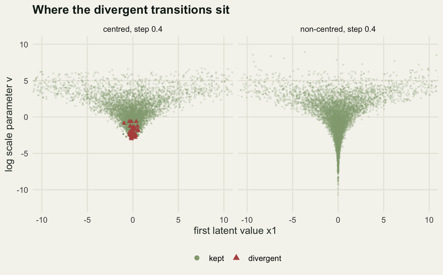

Figure 3: The log scale parameter against the first latent value, for the centred and non-centred parameterisations at the same step size. Divergent transitions (red triangles) occur only in the centred run and all of them sit in the lower half of the funnel, at the narrowest point the chain reached.

The horizontal axis is cut at plus and minus 10, which hides 344 of the centred draws and 362 of the non-centred ones, all of them at large values of the latent coordinate where the two panels agree anyway. What the picture shows is the part they disagree about: the left panel has a floor and the right one does not, and the red triangles sit on that floor.

Check four: Monte Carlo error against the decimals you report

The first three checks ask whether the sampler targeted the right distribution. The last one assumes it did and asks a different question: how many of the digits in the results table are real. A posterior mean reported to three decimal places makes a claim about the third one, and that claim is only supported if the Monte Carlo standard error is smaller than half a unit there.

target_mcse <- 0.0005; report_ess <- 200
ess_mean_need <- (post_sd / target_mcse)^2
need_q <- function(p) {
  q <- qbeta(p, post_a, post_b)
  p * (1 - p) / (target_mcse * dbeta(q, post_a, post_b))^2
}
mcse_q_at <- function(p, ess) {
  sqrt(p * (1 - p) / ess) / dbeta(qbeta(p, post_a, post_b), post_a, post_b)
}
prec_tab <- data.frame(
  quantity = c("posterior mean", "quantile 0.025", "quantile 0.5",
               "quantile 0.975"),
  ess_needed = round(c(ess_mean_need, need_q(0.025), need_q(0.5),
                       need_q(0.975))),
  mcse_at_report_ess = round(c(post_sd / sqrt(report_ess),
                               mcse_q_at(0.025, report_ess),
                               mcse_q_at(0.5, report_ess),
                               mcse_q_at(0.975, report_ess)), 5))
prec_tab$factor_vs_mean <- round(prec_tab$ess_needed / ess_mean_need, 2)
print(prec_tab)

        quantity ess_needed mcse_at_report_ess factor_vs_mean
1 posterior mean      54422            0.00825           1.00
2 quantile 0.025     117347            0.01211           2.16
3   quantile 0.5      92374            0.01075           1.70
4 quantile 0.975     536553            0.02590           9.86

need_norm <- function(p) p * (1 - p) * post_sd^2 / (target_mcse * dnorm(qnorm(p)))^2
print(round(c(target_mcse = target_mcse, report_ess = report_ess,
              post_sd = post_sd, ess_achieved = conv$ess[1],
              shortfall_mean = ess_mean_need / conv$ess[1],
              normal_tail_factor = need_norm(0.025) / ess_mean_need), 4))

       target_mcse         report_ess            post_sd       ess_achieved 
            0.0005           200.0000             0.1166         16210.0000 
    shortfall_mean normal_tail_factor 
            3.3573             7.1359 

The posterior standard deviation is 0.1166, so a Monte Carlo standard error of 0.0005 for the mean needs an effective sample size of 54422. The correct sampler from the first section, four chains of 12000 iterations on a one-parameter model, achieved 16210. That is short by a factor of 3.3573, on the easiest posterior anyone will ever sample, with 40000 draws in hand.

At the effective sample size of 200 that gets quoted as adequate, the Monte Carlo standard error of the mean is 0.00825. That is not a third decimal problem. The second decimal is already uncertain, so the reported 0.28623 supports two significant figures and no more, and any sentence in the abstract that turns on the third decimal has no support in the computation at all.

Now the tails, and this is where the obvious expectation breaks. The conventional advice is that quantiles far from the centre need far more draws than the mean, because there is less data out there. The measured factors say something more specific. The 0.025 quantile needs 117347, a factor of 2.16 over the mean. The 0.975 quantile needs 536553, a factor of 9.86. The two tails of the same posterior differ from each other by more than fourfold, and the cheaper one is only about twice the cost of the mean.

The reason is in the formula. The standard error of a quantile is inversely proportional to the posterior density at that quantile, and this posterior is skewed: it piles up against zero, so the density at the 0.025 quantile is high and the quantile is well determined, while the long right tail leaves the density at the 0.975 quantile low and the quantile loose. For a symmetric posterior with the same standard deviation, both tails cost a factor of 7.1359, identical by construction.

p_grid <- seq(0.01, 0.99, by = 0.005)
d4 <- rbind(
  data.frame(p = p_grid, need = need_q(p_grid), shape = "beta posterior (actual)"),
  data.frame(p = p_grid, need = need_norm(p_grid),
             shape = "normal with the same SD"))

ggplot(d4, aes(p, need, colour = shape, linetype = shape)) +
  geom_line(linewidth = 0.8) +
  geom_hline(yintercept = ess_mean_need, colour = te_pal$ink,
             linetype = 3, linewidth = 0.5) +
  annotate("text", x = 0.5, y = ess_mean_need * 0.72,
           label = "what the posterior mean needs",
           colour = "#2c3a31", size = 3.2) +
  annotate("point", x = c(0.025, 0.975),
           y = c(need_q(0.025), need_q(0.975)),
           size = 3, colour = te_pal$gold) +
  scale_y_log10(breaks = c(1e4, 3e4, 1e5, 3e5, 1e6),
                labels = c("10k", "30k", "100k", "300k", "1M")) +
  scale_colour_manual(values = c(`beta posterior (actual)` = te_pal$forest,
                                 `normal with the same SD` = te_pal$clay)) +
  labs(x = "quantile level", y = "effective sample size needed",
       colour = NULL, linetype = NULL,
       title = "Cost of a third decimal place, by quantile") +
  theme_te()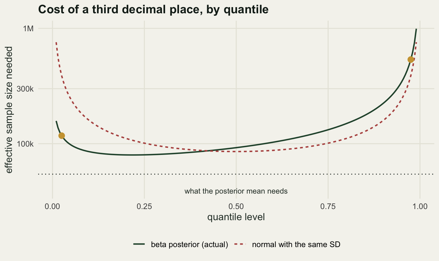

Figure 4: Effective sample size needed for a Monte Carlo standard error of 0.0005, as a function of quantile level, for the actual beta posterior and for a normal with the same standard deviation. Gold points mark the 0.025 and 0.975 quantiles of the beta; the dotted line is what the posterior mean needs.

The practical version of this is a habit rather than a rule. Before reporting a number, compute its Monte Carlo standard error and round the number to that error. If the standard error of the upper credible limit is 0.02590, then the limit gets two decimal places and no more, and anyone reading the table knows what the computation supports. The alternative, which is what most tables do, is to print whatever summary handed back and let the reader assume it is all signal.

What to take away

The four checks are not alternatives. Each one sees a failure the others do not. The exact benchmark caught the Jacobian bug at -32.38 standard errors and named the wrong target it was hitting, but it needs a model with a closed-form posterior, which the real analysis does not have. Simulation-based calibration works without one, scoring 15.36 on the correct sampler and 56.24 on the broken one, but it costs 400 fits and it told us the shape was a U when the cause was a data-dependent shift rather than underdispersion. The divergence and energy diagnostics caught a geometry failure that R-hat scored at 1.0631, which passes the threshold half the literature still quotes, and among those two the energy fraction was the one that kept failing after the divergence rate had been quieted to 0.0000 by a smaller step size while the answer stayed wrong at 2.3908 against a true 3. Monte Carlo standard error then told us how many digits of the survivor are real, and the answer for a chain with an effective sample size of 200 was fewer than two decimals.

If only one of the four fits into the time available, run the exact benchmark. It is the cheapest, it runs on the same code path as the real model, and the class of bug it catches, silently sampling a distribution that is not your posterior, is the class that no amount of chain-watching finds.

The honest limit is that all four checks here were run on toys: a one-parameter conjugate model with an answer in closed form and a ten-parameter funnel whose true marginals are known, and on a real hierarchical model there is no exact posterior to benchmark against, simulation-based calibration costs one full fit per replicate rather than the seconds it costs here, the quantile standard errors need a density estimated from the same chain being tested, and the thinning that makes the ranks independent is approximate rather than exact.

References

Gelman A, Rubin DB 1992 Statistical Science 7(4):457-472 (10.1214/ss/1177011136)

Geyer CJ 1992 Statistical Science 7(4):473-483 (10.1214/ss/1177011137)

Cook SR, Gelman A, Rubin DB 2006 Journal of Computational and Graphical Statistics 15(3):675-692 (10.1198/106186006X136976)

Talts S, Betancourt M, Simpson D, Vehtari A, Gelman A 2018 arXiv preprint (10.48550/arXiv.1804.06788)

Betancourt M 2016 arXiv preprint (10.48550/arXiv.1604.00695)

Flegal JM, Haran M, Jones GL 2008 Statistical Science 23(2):250-260 (10.1214/08-STS257)

Vehtari A, Gelman A, Simpson D, Carpenter B, Buerkner PC 2021 Bayesian Analysis 16(2):667-718 (10.1214/20-BA1221)

Related tutorials

• Hamiltonian Monte Carlo from scratch
• The Laplace approximation in R
• Reparameterisation and Neal’s funnel
• MCMC convergence diagnostics from scratch