library(ggplot2)

te_pal <- list(forest = "#275139", green = "#2f8f63", sage = "#93a87f",
               clay = "#b5534e", gold = "#cda23f", line = "#dad9ca",
               ink = "#16241d", paper = "#f5f4ee")

theme_te <- function() {
  theme_minimal(base_size = 12) +
    theme(panel.grid.minor = element_blank(),
          panel.grid.major = element_line(colour = "#e7e6dc"),
          plot.background = element_rect(fill = "#f5f4ee", colour = NA),
          panel.background = element_rect(fill = "#f5f4ee", colour = NA),
          plot.title = element_text(face = "bold", colour = te_pal$ink),
          axis.title = element_text(colour = "#2c3a31"),
          legend.position = "bottom")
}Hamiltonian Monte Carlo from scratch
R
MCMC
Bayesian statistics
ecology tutorial
Build Hamiltonian Monte Carlo in base R: leapfrog integration, energy error, and a measured comparison with random-walk Metropolis on a collinear posterior.
The two numbers came off the same hemispherical photograph. Canopy openness is the fraction of sky visible through a gap fraction analysis; transmitted light is the modelled radiation reaching the forest floor, computed from the same pixels with a solar track laid over them. Across sixty plots in a beech stand they correlate at better than 0.99, because one is essentially a smooth function of the other. Both went into a model of understorey herb biomass, because the field protocol said to record both and nobody revisited that until somebody tried to fit the thing.
That model is an unpleasant target to sample. The posterior is not diffuse, it is a narrow diagonal blade: the sum of the two coefficients is pinned down tightly by the data while their difference is barely constrained at all. A random-walk sampler dropped into that blade has to take short steps, because any step long enough to be useful along the blade is long enough to walk off the edge of it. It shuffles. You come back later to a trace plot that looks like a mountain range and an effective sample size in the dozens.
Stan does not shuffle here, and the reason is that Stan is not proposing at random. It builds a physical trajectory: it treats minus the log posterior as a potential energy landscape, gives the parameter vector a random shove, and rolls it across that landscape for a while under Hamilton’s equations. A ball rolling along the floor of a narrow valley follows the valley. That is the whole idea, and it fits in about forty lines of base R.
This post writes those lines and then measures what they buy: the potential energy, the Gaussian momentum, the leapfrog integrator, and the Metropolis correction that repairs the integrator’s error. Every claim is checked against something. The integrator is checked against exact reversibility and exact volume preservation, the sampler against a posterior whose mean, variance and correlation are known in closed form, and the efficiency against a random-walk sampler with both tuned and both counted in evaluations rather than in iterations. Some of what comes out is not what the folklore says.
If you have not built the random-walk sampler by hand, Metropolis-Hastings from scratch does that, and this post reuses its accept step almost verbatim. MCMC convergence diagnostics from scratch builds the effective sample size estimator that every efficiency number here depends on, and Gibbs sampling for conjugate models covers the case where you can sample the conditionals exactly and need none of this.
The survey, and a posterior we can check against
The model is deliberately one whose answer we already know. Log herb biomass, centred, regressed on two standardised canopy variables with a known residual standard deviation and an independent normal prior on each coefficient. With sigma fixed, that posterior is exactly bivariate normal, and its mean and covariance come out of two lines of matrix algebra. Everything the sampler produces later can be held against those two lines.
The predictors are built to be collinear on purpose, because collinearity is the condition under which gradient information starts to matter.
set.seed(20260728)
n_plot    <- 60
sigma_obs <- 0.35
tau_prior <- 5

open_c <- rnorm(n_plot)
light  <- 0.99 * open_c + sqrt(1 - 0.99^2) * rnorm(n_plot)
open_c <- (open_c - mean(open_c)) / sd(open_c)
light  <- (light  - mean(light))  / sd(light)
Xmat   <- cbind(open_c, light)
b_true <- c(0.45, 0.25)
yobs   <- drop(Xmat %*% b_true) + rnorm(n_plot, 0, sigma_obs)
yobs   <- yobs - mean(yobs)

Prec  <- crossprod(Xmat) / sigma_obs^2 + diag(2) / tau_prior^2
Covp  <- solve(Prec)
mpost <- unname(drop(Covp %*% (crossprod(Xmat, yobs) / sigma_obs^2)))
sd_post  <- unname(sqrt(diag(Covp)))
cor_post <- unname(Covp[1, 2] / prod(sd_post))
axis_sd  <- sqrt(eigen(Covp, symmetric = TRUE)$values)
axis_vec <- eigen(Covp, symmetric = TRUE)$vectors
eps_lim  <- 2 * min(axis_sd)

print(round(c(plots = n_plot, sigma = sigma_obs, prior_sd = tau_prior,
              predictor_r = cor(open_c, light)), 4))
plots sigma prior_sd predictor_r
60.0000 0.3500 5.0000 0.9943 print(round(c(true_open = b_true[1], true_light = b_true[2],
post_mean_open = mpost[1], post_mean_light = mpost[2],
post_mean_sum = sum(mpost), true_sum = sum(b_true)), 4)) true_open true_light post_mean_open post_mean_light post_mean_sum
0.4500 0.2500 0.0060 0.7123 0.7183
true_sum
0.7000 print(round(c(post_sd_open = sd_post[1], post_sd_light = sd_post[2],
post_corr = cor_post), 4)) post_sd_open post_sd_light post_corr
0.4231 0.4231 -0.9942 print(round(c(along_ridge_sd = max(axis_sd), across_ridge_sd = min(axis_sd),
axis_ratio = max(axis_sd) / min(axis_sd), eps_limit = eps_lim), 4)) along_ridge_sd across_ridge_sd axis_ratio eps_limit
0.5975 0.0323 18.5184 0.0645 The two predictors correlate at 0.9943 in this sample, and the posterior inherits the mirror image of that: the coefficients correlate at -0.9942. Look at what this does to the individual estimates. The true coefficients were 0.4500 and 0.2500, and the posterior means are 0.0060 and 0.7123, which the data pin down only in combination. The sum is fine: the truth is 0.7000 and the posterior mean of the sum is 0.7183. This is what collinearity does. The data speak clearly about the combined effect of the two canopy variables and say almost nothing about how to split it between them, and the posterior is honest about that by being long in one direction and thin in the other.
The last line puts numbers on the shape. Rotating the posterior onto its own principal axes, the standard deviation along the ridge is 0.5975 and the standard deviation across it is 0.0323, a ratio of 18.5184. Any sampler that takes isotropic steps is caught between those two numbers: the across-ridge width sets how far it can safely step, the along-ridge length sets how far it needs to travel. The quantity called eps_limit, twice the across-ridge standard deviation, will turn out to be exactly where the leapfrog integrator falls apart. Hold onto 0.0645 for two sections.
Potential energy, momentum, and a gradient written by hand
Hamiltonian Monte Carlo starts by renaming things. The negative log posterior becomes a potential energy \(U(q)\), where \(q\) is the parameter vector. Then it invents a momentum vector \(p\) of the same length, gives it an independent standard normal distribution, and calls \(K(p) = \frac{1}{2}p^{\top}p\) the kinetic energy. The joint density of \((q, p)\) is proportional to \(\exp(-U(q) - K(p))\), and because the two blocks are independent, the marginal of \(q\) under that joint density is exactly the posterior we wanted. The momentum is scaffolding. It is thrown away after every iteration and drawn fresh.
For this model the potential is a sum of squares over the residuals plus a ridge term from the prior, and the gradient is one line of matrix algebra: \(\nabla U(b) = -X^{\top}(y - Xb)/\sigma^2 + b/\tau^2\). Writing it out and pre-computing the cross-products means a gradient costs one small matrix product, the same order of work as evaluating the potential itself. That matters later, when we start counting.
XtX <- crossprod(Xmat)
Xty <- unname(drop(crossprod(Xmat, yobs)))
yty <- sum(yobs * yobs)

pot <- function(b) {
  (yty - 2 * sum(b * Xty) + sum(b * (XtX %*% b))) / (2 * sigma_obs^2) +
    sum(b * b) / (2 * tau_prior^2)
}
grad_pot <- function(b) {
  (drop(XtX %*% b) - Xty) / sigma_obs^2 + b / tau_prior^2
}

b_chk  <- c(0.20, 0.70)
step_h <- 1e-6
g_hand <- unname(grad_pot(b_chk))
g_num  <- c((pot(b_chk + c(step_h, 0)) - pot(b_chk - c(step_h, 0))) / (2 * step_h),
            (pot(b_chk + c(0, step_h)) - pot(b_chk - c(0, step_h))) / (2 * step_h))
g_quad <- unname(drop(Prec %*% (b_chk - mpost)))

print(round(c(gradient_1 = g_hand[1], gradient_2 = g_hand[2]), 2))
gradient_1 gradient_2
87.57 86.99 print(signif(c(fd_step = step_h,
vs_finite_difference = max(abs(g_hand - g_num)),
vs_quadratic_form = max(abs(g_hand - g_quad))), 4)) fd_step vs_finite_difference vs_quadratic_form
1.000e-06 1.446e-08 3.894e-12 Two checks on the same gradient, because a wrong gradient is the commonest way to get an HMC implementation that runs happily and samples the wrong distribution. At the test point the analytic gradient is 87.57 and 86.99. A central finite difference of the potential with a step of 1.000e-06 agrees to 1.446e-08, which is about what you expect once floating point cancellation is accounted for. The quadratic form \(\Lambda(b - m)\), which is what the gradient of a Gaussian potential must reduce to, agrees to 3.894e-12, which is machine precision.
Do this check on your own models: it costs four lines, and if the two numbers disagree, nothing downstream is worth reading.
The leapfrog, and why it has to be reversible
Hamilton’s equations say that \(\dot{q} = p\) and \(\dot{p} = -\nabla U(q)\). Solving them exactly is not on offer for a real posterior, so we integrate numerically, and the choice of integrator is not free. The Metropolis correction that makes HMC exact requires the proposal map to be reversible and to preserve volume in phase space. Ordinary Runge-Kutta does neither. The leapfrog scheme does both, and it does them exactly rather than approximately.
Its structure is a half step on the momentum, a full step on the position, and a half step on the momentum again. Consecutive half steps in the middle of a trajectory merge, so a trajectory of \(L\) position updates costs \(L + 1\) gradient evaluations, and that is the number this post counts.
leapfrog <- function(q, p, eps, n_step, grad_fun) {
  p <- p - 0.5 * eps * grad_fun(q)
  for (i in seq_len(n_step)) {
    q <- q + eps * p
    if (i < n_step) p <- p - eps * grad_fun(q)
  }
  list(q = q, p = p - 0.5 * eps * grad_fun(q))
}

q_start <- c(0.10, 0.80)
p_start <- c(-0.40, 1.10)
fwd <- leapfrog(q_start, p_start, 0.045, 30, grad_pot)
bck <- leapfrog(fwd$q, -fwd$p, 0.045, 30, grad_pot)
print(signif(c(position_returned = max(abs(bck$q - q_start)),
               momentum_returned = max(abs(-bck$p - p_start))), 3))
position_returned momentum_returned
1.11e-15 3.33e-16 flow <- function(z) {
r <- leapfrog(z[1:2], z[3:4], 0.045, 30, grad_pot)
c(r$q, r$p)
}
jac <- matrix(0, 4, 4)
for (j in 1:4) {
bump <- rep(0, 4); bump[j] <- 1e-5
jac[, j] <- (flow(c(q_start, p_start) + bump) -
flow(c(q_start, p_start) - bump)) / 2e-5
}
print(round(c(jacobian_determinant = det(jac)), 6))jacobian_determinant
1 print(signif(c(distance_from_one = abs(det(jac) - 1)), 4))distance_from_one
8.148e-11 The reversibility test is the honest one: run thirty leapfrog steps forwards, flip the sign of the momentum, run thirty more, and see where you are. If the integrator is reversible you are back at the start. The position returns to within 1.11e-15 and the momentum to within 3.33e-16. Those are rounding errors accumulated over sixty steps, not integration errors. The map really is its own inverse once you negate the momentum.
Volume preservation is checked by building the Jacobian of the whole four-dimensional map with central differences and taking its determinant. It comes out at 1, away from one by 8.148e-11, which is the accuracy of the finite difference rather than a property of the integrator. A phase-space volume carried along by the leapfrog is squeezed and sheared but never compressed. That is why the accept ratio in a later section is a plain ratio of joint densities with no Jacobian factor hanging off it.
Energy is not conserved, and that is the point
The exact Hamiltonian flow conserves \(H(q, p) = U(q) + K(p)\). The leapfrog does not. What it conserves instead is a nearby modified Hamiltonian, which is why its energy error stays bounded and oscillates rather than drifting away. The cleanest place to see this is a standard normal target, where \(U(q) = q^2/2\) and the exact flow is a circle in the \((q, p)\) plane. The leapfrog traces an ellipse instead, and the ellipse can be written down: starting from \(q = 1.5\) with zero momentum, the orbit reaches a maximum momentum of \(1.5\sqrt{1 - \varepsilon^2/4}\).
grad_std <- function(q) q

orbit <- function(eps, n_step, q0, p0) {
  qs <- numeric(n_step + 1); ps <- numeric(n_step + 1)
  qs[1] <- q0; ps[1] <- p0
  q <- q0; ph <- p0 - 0.5 * eps * grad_std(q0)
  for (i in seq_len(n_step)) {
    q <- q + eps * ph
    gq <- grad_std(q)
    qs[i + 1] <- q; ps[i + 1] <- ph - 0.5 * eps * gq
    ph <- ph - eps * gq
  }
  data.frame(q = qs, p = ps)
}

eps_orb <- c(0.3, 0.9, 1.8)
n_orb   <- 140
q_orb   <- 1.5
orb <- do.call(rbind, lapply(eps_orb, function(e) {
  o <- orbit(e, n_orb, q_orb, 0)
  o$eps <- factor(sprintf("%.1f", e))
  o
}))
shape <- do.call(rbind, lapply(eps_orb, function(e) {
  o <- orbit(e, n_orb, q_orb, 0)
  data.frame(eps = e, q_reach = max(abs(o$q)), p_reach = max(abs(o$p)),
             p_predicted = q_orb * sqrt(1 - e^2 / 4))
}))
print(round(shape, 4))
eps q_reach p_reach p_predicted
1 0.3 1.5 1.4830 1.4830
2 0.9 1.5 1.3395 1.3395
3 1.8 1.5 0.6538 0.6538print(round(c(orbit_steps = n_orb, start_position = q_orb,
step_small = eps_orb[1], step_mid = eps_orb[2],
step_large = eps_orb[3]), 2)) orbit_steps start_position step_small step_mid step_large
140.0 1.5 0.3 0.9 1.8 All three orbits reach the same maximum position, 1.5, because that is where they started with no momentum. What differs is how far up the momentum axis they get. At a step size of 0.3 the orbit reaches 1.4830 and the prediction is 1.4830. At 1.8 it reaches only 0.6538 against a prediction of 0.6538. The orbits stay closed, which is the bounded error, but the large-step orbit is a flattened ellipse rather than the circle the exact flow would trace.
ang  <- seq(0, 2 * pi, length.out = 400)
ring <- data.frame(q = q_orb * cos(ang), p = q_orb * sin(ang))

ggplot(orb, aes(q, p, colour = eps)) +
  geom_point(size = 0.9) +
  geom_path(data = ring, aes(q, p), inherit.aes = FALSE,
            colour = te_pal$ink, linetype = "dashed", linewidth = 0.45) +
  scale_colour_manual(values = c("0.3" = te_pal$green, "0.9" = te_pal$gold,
                                 "1.8" = te_pal$clay),
                      name = "leapfrog step size") +
  coord_fixed(xlim = c(-1.75, 1.75), ylim = c(-1.75, 1.75)) +
  labs(x = "position q", y = "momentum p",
       title = "Leapfrog orbits in phase space") +
  theme_te()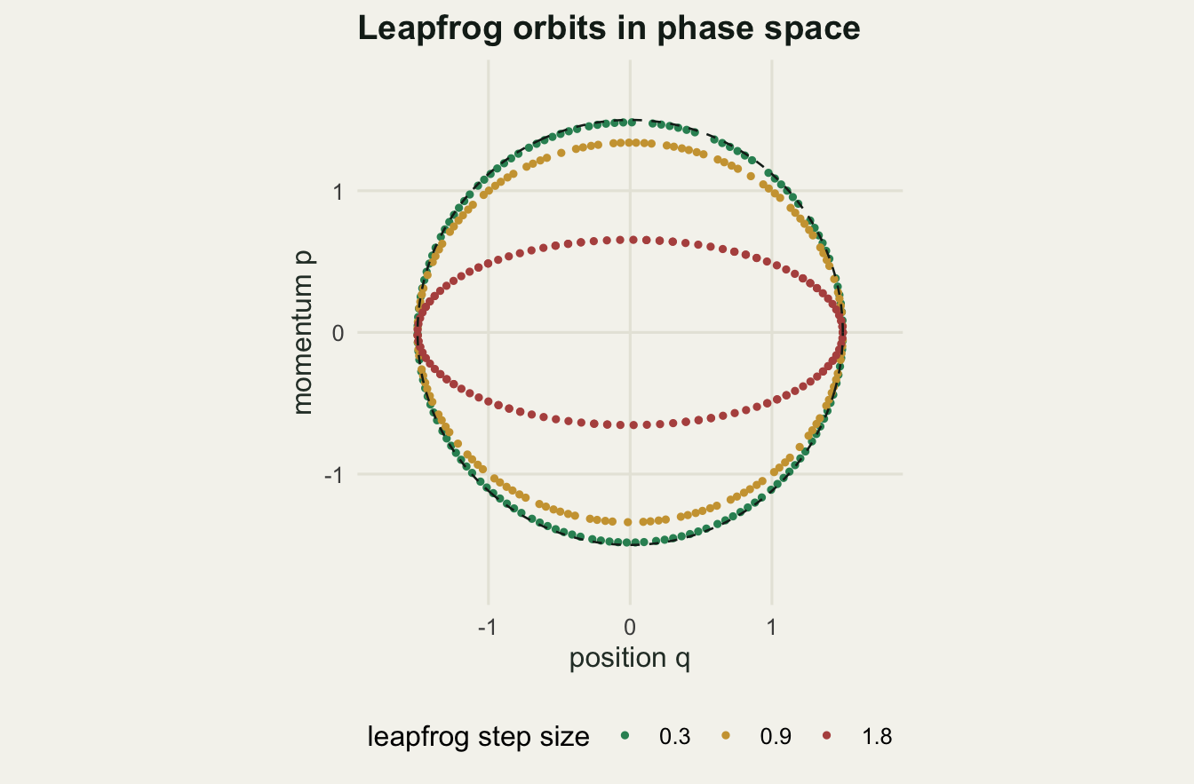
The flattening has a limit. When the step size reaches 2 on this target the predicted momentum reach hits zero and the quantity under the square root turns negative, which is the algebra telling you the orbit has stopped being an ellipse and become a hyperbola. Past that point the trajectory never comes back: it runs off to infinity, geometrically.
Sweeping the step size until the integrator breaks
On the collinear posterior the same threshold applies, scaled by the tightest direction of the target. The across-ridge standard deviation is 0.0323, so the prediction is that the leapfrog holds together up to a step size of about 0.0645 and disintegrates after it. The sweep below fixes the trajectory at 12 steps, runs 400 proposals at each of 14 step sizes, and records the acceptance rate and the mean absolute change in the Hamiltonian.
eps_grid <- c(0.010, 0.020, 0.030, 0.040, 0.050, 0.056, 0.060, 0.062,
              0.064, 0.066, 0.068, 0.070, 0.080, 0.100)
n_probe <- 400
sweep_eps <- data.frame(eps = eps_grid, accept = NA_real_, energy_error = NA_real_)

for (i in seq_along(eps_grid)) {
  set.seed(51000000 + i)
  ee <- eps_grid[i]; q <- mpost; taken <- 0L; err <- numeric(n_probe)
  for (r in seq_len(n_probe)) {
    p <- rnorm(2)
    st <- leapfrog(q, p, ee, 12, grad_pot)
    dh <- pot(st$q) + 0.5 * sum(st$p * st$p) - pot(q) - 0.5 * sum(p * p)
    err[r] <- dh
    if (is.finite(dh) && log(runif(1)) < -dh) { q <- st$q; taken <- taken + 1L }
  }
  sweep_eps$accept[i] <- taken / n_probe
  sweep_eps$energy_error[i] <- mean(abs(err))
}
sweep_eps$log10_error <- log10(sweep_eps$energy_error)

print(data.frame(eps = sweep_eps$eps, accept = round(sweep_eps$accept, 3),
                 log10_error = round(sweep_eps$log10_error, 2)))
eps accept log10_error
1 0.010 0.988 -2.08
2 0.020 0.975 -1.21
3 0.030 0.935 -0.85
4 0.040 0.955 -1.00
5 0.050 0.838 -0.35
6 0.056 0.953 -1.21
7 0.060 0.755 -0.19
8 0.062 0.600 0.18
9 0.064 0.850 -0.52
10 0.066 0.002 4.87
11 0.068 0.000 6.88
12 0.070 0.000 8.44
13 0.080 0.000 13.73
14 0.100 0.000 20.27print(round(c(probes_per_step_size = n_probe, steps_per_trajectory = 12,
last_stable_eps = max(sweep_eps$eps[sweep_eps$accept > 0.05]),
first_broken_eps = min(sweep_eps$eps[sweep_eps$accept <= 0.05]), predicted_limit = eps_lim), 4))probes_per_step_size steps_per_trajectory last_stable_eps
400.0000 12.0000 0.0640
first_broken_eps predicted_limit
0.0660 0.0645 The collapse is not gradual. At a step size of 0.064 the acceptance rate is 0.850 and the mean energy error is ten to the -0.52. One grid point later, at 0.066, acceptance is 0.002 and the energy error is ten to the 4.87. That is not a sampler mixing badly. That is a sampler whose every proposal has been thrown to infinity and rejected. The predicted threshold was 0.0645, and the measured break falls between 0.064 and 0.066, which brackets it.
Below the threshold the acceptance rate does not fall smoothly with the step size, and that is worth pausing on. It goes 0.838 at 0.050, up to 0.953 at 0.056, down to 0.600 at 0.062, and back up to 0.850 at 0.064. The number of steps is held at 12 here, so changing the step size also changes where in its orbit the trajectory stops, and the modified Hamiltonian the leapfrog conserves differs from the true one by an amount that depends on that phase. Tuning a step size by watching acceptance alone, on a short trajectory, can hand you a local optimum that means nothing.
sb <- rbind(
  data.frame(eps = sweep_eps$eps, value = sweep_eps$accept,
             panel = "acceptance rate"),
  data.frame(eps = sweep_eps$eps, value = sweep_eps$log10_error,
             panel = "log10 mean energy error"))

ggplot(sb, aes(eps, value)) +
  geom_vline(xintercept = eps_lim, colour = te_pal$clay, linetype = "dashed",
             linewidth = 0.6) +
  geom_line(colour = te_pal$forest, linewidth = 0.7) +
  geom_point(colour = te_pal$forest, size = 1.8) +
  facet_wrap(~panel, ncol = 1, scales = "free_y") +
  labs(x = "leapfrog step size", y = NULL,
       title = "The integrator breaks at a sharp step size") +
  theme_te()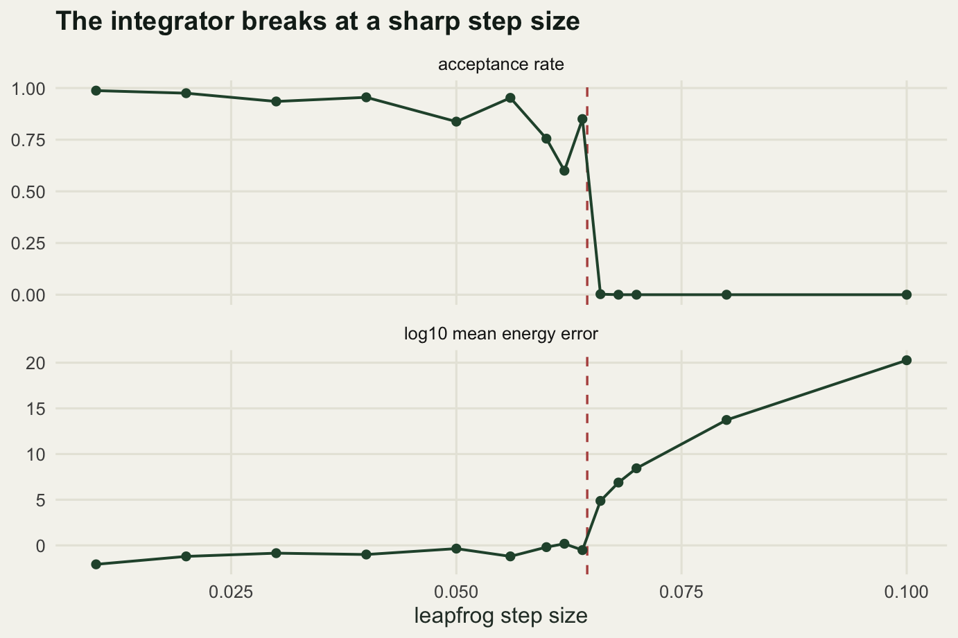
The lower panel is the more useful diagnostic in practice. Stan reports these overshoots as divergent transitions, and a divergence is exactly this: a trajectory whose energy error was large enough that the integrator is no longer tracking the dynamics. On a Gaussian target you can work the threshold out in advance. On a real hierarchical model you cannot, which is why the warning exists.
The accept step, and a check against the closed form
The integrator’s error is a bias, and the Metropolis correction removes it. After a trajectory from \((q, p)\) to \((q^{*}, p^{*})\), accept the new position with probability \(\min(1, \exp(H(q, p) - H(q^{*}, p^{*})))\). If the integration were exact the exponent would be zero and every proposal would be accepted; because it is not, the accept step converts energy error into rejections and the chain stays exactly on the target. There is no Jacobian term because the earlier section measured that the Jacobian is one.
The sampler and the effective sample size estimator both go in here. The autocovariances come out of an FFT, and the effective sample size uses Geyer’s initial positive sequence: sum the autocorrelations in adjacent pairs and stop at the first pair that is not positive. One property of that estimator matters below. It can never return more than the chain length, so when a sampler produces draws that are better than independent, which HMC on a Gaussian target routinely does, the number reported is a floor rather than the truth.
autocov <- function(x) {
  n <- length(x); x <- x - mean(x)
  n2 <- 2^ceiling(log2(2 * n))
  fx <- fft(c(x, rep(0, n2 - n)))
  Re(fft(fx * Conj(fx), inverse = TRUE))[seq_len(n)] / (n2 * n)
}

ess_series <- function(x) {
  n <- length(x); gam <- autocov(x)
  if (gam[1] <= 0) return(NA_real_)
  rho <- gam / gam[1]; k <- floor((n - 2) / 2)
  paired <- rho[2 * seq_len(k)] + rho[2 * seq_len(k) + 1]
  stop_at <- which(paired <= 0)
  m <- if (length(stop_at)) stop_at[1] - 1L else k
  n / (1 + 2 * (if (m >= 1) sum(paired[seq_len(m)]) else 0))
}

ess_worst <- function(draws) min(apply(draws, 2, ess_series))

hmc_chain <- function(q0, eps, n_step, n_iter, grad_fun, pot_fun, seed) {
  set.seed(seed)
  d <- length(q0)
  kicks <- matrix(rnorm(n_iter * d), n_iter, d)
  logu <- log(runif(n_iter)); keep <- matrix(0, n_iter, d)
  q <- q0; uq <- pot_fun(q); taken <- 0L
  for (it in seq_len(n_iter)) {
    p <- kicks[it, ]
    st <- leapfrog(q, p, eps, n_step, grad_fun)
    unew <- pot_fun(st$q)
    dh <- unew + 0.5 * sum(st$p * st$p) - uq - 0.5 * sum(p * p)
    if (is.finite(dh) && logu[it] < -dh) { q <- st$q; uq <- unew; taken <- taken + 1L }
    keep[it, ] <- q
  }
  list(draws = keep, accept = taken / n_iter, evals = n_iter * (n_step + 1))
}

rw_chain <- function(q0, scale_p, n_iter, pot_fun, seed) {
  set.seed(seed)
  d <- length(q0)
  jumps <- matrix(rnorm(n_iter * d, 0, scale_p), n_iter, d)
  logu <- log(runif(n_iter)); keep <- matrix(0, n_iter, d)
  q <- q0; uq <- pot_fun(q); taken <- 0L
  for (it in seq_len(n_iter)) {
    prop <- q + jumps[it, ]; unew <- pot_fun(prop)
    if (logu[it] < uq - unew) { q <- prop; uq <- unew; taken <- taken + 1L }
    keep[it, ] <- q
  }
  list(draws = keep, accept = taken / n_iter, evals = n_iter)
}
That is the whole sampler. The leapfrog and the accept loop together, and the only thing inside either that is not arithmetic is the call to the gradient. Now hold it against the closed form.
n_val  <- 4000
step_v <- 0.052
L_val  <- 29
val <- hmc_chain(mpost, step_v, L_val, n_val, grad_pot, pot, 60606060)

print(c(iterations = n_val, leapfrog_steps = L_val,
        gradient_evaluations = val$evals))
iterations leapfrog_steps gradient_evaluations
4000 29 120000 print(round(c(step_size = step_v, accept = val$accept), 4))step_size accept
0.0520 0.7415 print(round(c(mean_open_hmc = mean(val$draws[, 1]), mean_open_exact = mpost[1],
mean_light_hmc = mean(val$draws[, 2]), mean_light_exact = mpost[2]), 4)) mean_open_hmc mean_open_exact mean_light_hmc mean_light_exact
0.0122 0.0060 0.7049 0.7123 print(round(c(sd_open_hmc = sd(val$draws[, 1]), sd_open_exact = sd_post[1],
sd_light_hmc = sd(val$draws[, 2]), sd_light_exact = sd_post[2],
corr_hmc = cor(val$draws[, 1], val$draws[, 2]),
corr_exact = cor_post), 4)) sd_open_hmc sd_open_exact sd_light_hmc sd_light_exact corr_hmc
0.4243 0.4231 0.4232 0.4231 -0.9943
corr_exact
-0.9942 val_ess <- apply(val$draws, 2, ess_series)
mcse <- apply(val$draws, 2, sd) / sqrt(val_ess)
print(round(c(ess_open = val_ess[1], ess_light = val_ess[2]), 1)) ess_open ess_light
4000 4000 print(round(c(mcse_open = mcse[1], mcse_light = mcse[2],
error_open = mean(val$draws[, 1]) - mpost[1],
error_light = mean(val$draws[, 2]) - mpost[2]), 4)) mcse_open mcse_light error_open error_light
0.0067 0.0067 0.0062 -0.0074 4000 iterations at a step size of 0.052 with 29 leapfrog steps, which is 120000 gradient evaluations, accepting 0.7415 of proposals. The posterior mean of the first coefficient is 0.0060 exactly and 0.0122 from the chain. The second is 0.7123 exactly and 0.7049 from the chain. The standard deviations are 0.4231 and 0.4231 exactly against 0.4243 and 0.4232. The correlation is -0.9942 exactly against -0.9943.
The errors on the two means are 0.0062 and -0.0074, and the Monte Carlo standard error on the first of the two is 0.0067. The effective sample size for the first coefficient came back as 4000, because at this trajectory length successive draws carry little autocorrelation. The truth is at least that good.
What the gradients buy, counted in evaluations
Here is the comparison that justifies the whole apparatus, and it has to be done carefully or it means nothing. Comparing HMC and random-walk Metropolis per iteration is meaningless, because one HMC iteration costs n_step + 1 gradient evaluations and one random-walk iteration costs one potential evaluation. The currency has to be work. For this model a gradient and a potential evaluation are both one small matrix product, so counting them one for one is close to fair; that assumption is revisited below, and it does not survive intact.
Both samplers are tuned on a fixed budget of 30000 evaluations. The HMC grid crosses four step sizes with three trajectory lengths; the random-walk grid runs seven proposal scales spanning a factor of more than twenty.
budget <- 30000
hmc_tune <- data.frame(eps = rep(c(0.032, 0.045, 0.052, 0.058), each = 3),
                       traj = rep(c(0.95, 1.5, 2.2), times = 4))
hmc_tune$n_step <- pmax(1, round(hmc_tune$traj / hmc_tune$eps))
hmc_tune$iters  <- floor(budget / (hmc_tune$n_step + 1))
hmc_tune$accept <- NA_real_; hmc_tune$ess_per_eval <- NA_real_
for (i in seq_len(nrow(hmc_tune))) {
  r <- hmc_chain(mpost, hmc_tune$eps[i], hmc_tune$n_step[i], hmc_tune$iters[i],
                 grad_pot, pot, 31415926)
  hmc_tune$accept[i] <- r$accept
  hmc_tune$ess_per_eval[i] <- ess_worst(r$draws) / r$evals
}
print(data.frame(eps = hmc_tune$eps, n_step = hmc_tune$n_step,
                 iters = hmc_tune$iters, accept = round(hmc_tune$accept, 3),
                 ess_per_eval = round(hmc_tune$ess_per_eval, 5)))
eps n_step iters accept ess_per_eval
1 0.032 30 967 0.978 0.02779
2 0.032 47 625 0.923 0.02083
3 0.032 69 428 0.944 0.01429
4 0.045 21 1363 0.814 0.03159
5 0.045 33 882 0.861 0.02941
6 0.045 49 600 0.953 0.02000
7 0.052 18 1578 0.766 0.03024
8 0.052 29 1000 0.740 0.03333
9 0.052 42 697 0.943 0.02326
10 0.058 16 1764 0.552 0.02350
11 0.058 26 1111 0.516 0.03585
12 0.058 38 769 0.978 0.02564rw_tune <- data.frame(scale_mult = c(1.7, 3.6, 7, 14, 20, 28, 40))
rw_tune$scale_p <- rw_tune$scale_mult * min(axis_sd)
rw_tune$accept <- NA_real_; rw_tune$ess_per_eval <- NA_real_
for (i in seq_len(nrow(rw_tune))) {
r <- rw_chain(mpost, rw_tune$scale_p[i], budget, pot, 27182818)
rw_tune$accept[i] <- r$accept
rw_tune$ess_per_eval[i] <- ess_worst(r$draws) / r$evals
}
print(data.frame(mult = rw_tune$scale_mult, scale = round(rw_tune$scale_p, 4),
accept = round(rw_tune$accept, 3),
ess_per_eval = round(rw_tune$ess_per_eval, 5))) mult scale accept ess_per_eval
1 1.7 0.0549 0.554 0.00150
2 3.6 0.1162 0.320 0.00425
3 7.0 0.2259 0.169 0.00358
4 14.0 0.4517 0.081 0.01021
5 20.0 0.6453 0.051 0.01045
6 28.0 0.9034 0.033 0.01167
7 40.0 1.2906 0.019 0.01008ih <- which.max(hmc_tune$ess_per_eval)
ir <- which.max(rw_tune$ess_per_eval)
print(round(c(budget_evaluations = budget,
hmc_best = hmc_tune$ess_per_eval[ih],
hmc_accept = hmc_tune$accept[ih],
rw_best = rw_tune$ess_per_eval[ir],
rw_accept = rw_tune$accept[ir],
hmc_over_rw = hmc_tune$ess_per_eval[ih] / rw_tune$ess_per_eval[ir],
classic_rw_target = 0.234), 4))budget_evaluations hmc_best hmc_accept rw_best
30000.0000 0.0358 0.5158 0.0117
rw_accept hmc_over_rw classic_rw_target
0.0331 3.0711 0.2340 The best HMC setting delivers 0.0358 effective draws per gradient evaluation, at 26 leapfrog steps and a step size of 0.058. The best random walk delivers 0.0117 per potential evaluation. The ratio is 3.0711.
Three per unit of work, on a posterior with a correlation of -0.9942 and an axis ratio of 18.5184. That is a real gain and it is not the order of magnitude the folklore promises. The reason is visible in the random-walk table. The scale that wins is 0.9034, which is 28 times the across-ridge standard deviation and larger than the along-ridge standard deviation, and it accepts 0.0331 of its proposals. The textbook target acceptance for random-walk Metropolis is 0.234. The best tuning here is nowhere near it: the sampler does better by throwing enormous proposals, having almost all of them rejected, and occasionally landing a jump that crosses the entire ridge in one move. In two dimensions a huge proposal still has a workable chance of landing on the blade. That trick is what keeps the random walk competitive here, and it is also the trick that dies as soon as the problem gets bigger, which the dimension sweep in the next section shows.
cloud_hmc <- hmc_chain(mpost, hmc_tune$eps[ih], hmc_tune$n_step[ih],
                       floor(budget / (hmc_tune$n_step[ih] + 1)),
                       grad_pot, pot, 12211221)
cloud_rw  <- rw_chain(mpost, rw_tune$scale_p[ir], budget, pot, 13311331)
thin_by  <- hmc_tune$n_step[ih] + 1
thin_idx <- seq(1, budget, by = thin_by)

lab_h <- sprintf("HMC: %d draws, worst ESS %.0f", nrow(cloud_hmc$draws), ess_worst(cloud_hmc$draws))
lab_r <- sprintf("Random walk: %d draws, worst ESS %.0f", length(thin_idx), ess_worst(cloud_rw$draws))
cl <- rbind(
  data.frame(b1 = cloud_hmc$draws[, 1], b2 = cloud_hmc$draws[, 2], who = lab_h),
  data.frame(b1 = cloud_rw$draws[thin_idx, 1], b2 = cloud_rw$draws[thin_idx, 2], who = lab_r))
cl$who <- factor(cl$who, levels = c(lab_h, lab_r))

ell <- axis_vec %*% diag(axis_sd * sqrt(qchisq(0.95, 2))) %*% rbind(cos(ang), sin(ang))
ell <- data.frame(b1 = mpost[1] + ell[1, ], b2 = mpost[2] + ell[2, ])

print(round(c(ellipse_percent = 95, cloud_hmc_points = nrow(cloud_hmc$draws),
              cloud_rw_points = length(thin_idx),
              cloud_hmc_ess = ess_worst(cloud_hmc$draws),
              cloud_rw_ess = ess_worst(cloud_rw$draws)), 1))
ellipse_percent cloud_hmc_points cloud_rw_points cloud_hmc_ess
95.0 1111.0 1112.0 721.0
cloud_rw_ess
271.1 ggplot(cl, aes(b1, b2)) +
geom_point(colour = te_pal$green, alpha = 0.4, size = 0.85) +
geom_path(data = ell, aes(b1, b2), inherit.aes = FALSE,
colour = te_pal$clay, linewidth = 0.7) +
facet_wrap(~who) +
labs(x = "coefficient on canopy openness", y = "coefficient on light",
title = "Same evaluation budget, two samplers") +
theme_te()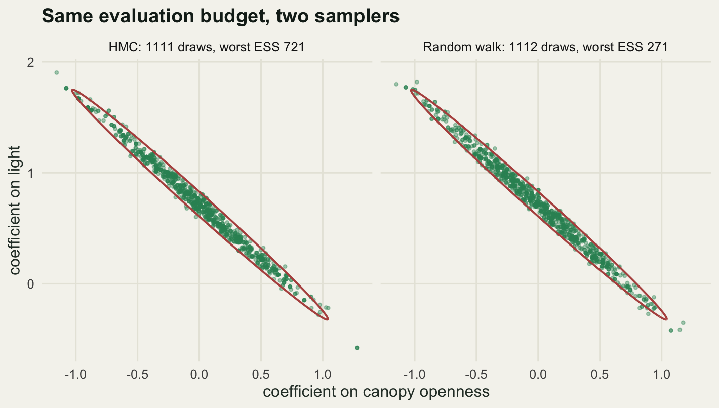
The picture is worth looking at precisely because the two clouds are so similar. Both cover the ridge, both fill the exact 95 per cent ellipse and spill a little past it, and neither shape tells you which sampler was better. The difference is in the counting: 721.0 effective draws for HMC against 271.1 for the random walk, from the same 30000 evaluations. Judging a sampler by looking at its scatter plot is not a method.
Where the gain actually comes from
Two dimensions is a small problem. To find out where the gain lives, run the same tuned comparison on plain Gaussian targets: first sweeping the correlation at two dimensions, then sweeping the dimension with no correlation at all. Both samplers get a small tuning grid each time and the best of each is reported.
gauss_target <- function(Sig) {
  Pm <- solve(Sig)
  list(pot = function(q) 0.5 * sum(q * (Pm %*% q)),
       grad = function(q) drop(Pm %*% q),
       dim = nrow(Sig), ax = sqrt(eigen(Sig, symmetric = TRUE)$values))
}
tune_rw <- function(tg, n_iter, seed) {
  best <- c(eff = -1, acc = NA)
  for (f in c(2.4, 6, 14, 30)) {
    r <- rw_chain(rep(0, tg$dim), f * min(tg$ax) / sqrt(tg$dim), n_iter, tg$pot, seed)
    e <- ess_worst(r$draws) / r$evals
    if (!is.na(e) && e > best["eff"]) best <- c(eff = e, acc = r$accept)
  }
  best
}
tune_hmc <- function(tg, n_iter, seed) {
  best <- c(eff = -1, acc = NA, nstep = NA)
  for (ef in c(0.3, 0.55, 0.85)) for (tf in c(0.7, 1.3)) {
    e <- ef * 2 * min(tg$ax)
    L <- max(1, round(tf * (pi / 2) * max(tg$ax) / e))
    r <- hmc_chain(rep(0, tg$dim), e, L, n_iter, tg$grad, tg$pot, seed)
    ee <- ess_worst(r$draws) / r$evals
    if (!is.na(ee) && ee > best["eff"]) best <- c(eff = ee, acc = r$accept, nstep = L)
  }
  best
}

corr_grid <- c(0, 0.9, 0.99)
corr_out <- data.frame(correlation = corr_grid, rw = NA_real_, hmc = NA_real_,
                       steps = NA_real_, gain = NA_real_)
for (i in seq_along(corr_grid)) {
  tg <- gauss_target(matrix(c(1, corr_grid[i], corr_grid[i], 1), 2, 2))
  a <- tune_rw(tg, 15000, 4040404)
  b <- tune_hmc(tg, 2500, 5050505)
  corr_out$rw[i]    <- unname(a["eff"])
  corr_out$hmc[i]   <- unname(b["eff"])
  corr_out$steps[i] <- unname(b["nstep"])
  corr_out$gain[i]  <- unname(b["eff"] / a["eff"])
}
print(data.frame(correlation = corr_out$correlation, rw = round(corr_out$rw, 5),
                 hmc = round(corr_out$hmc, 5), steps = corr_out$steps,
                 gain = round(corr_out$gain, 2)))
correlation rw hmc steps gain
1 0.00 0.12319 0.33333 2 2.71
2 0.90 0.04939 0.13225 5 2.68
3 0.99 0.01631 0.05556 17 3.41print(round(c(rw_penalty = corr_out$rw[1] / corr_out$rw[3],
hmc_penalty = corr_out$hmc[1] / corr_out$hmc[3]), 3)) rw_penalty hmc_penalty
7.555 6.000 dim_grid <- c(1, 2, 5, 10, 25)
dim_out <- data.frame(dimension = dim_grid, rw = NA_real_, hmc = NA_real_,
gain = NA_real_)
for (i in seq_along(dim_grid)) {
tg <- gauss_target(diag(dim_grid[i]))
a <- tune_rw(tg, 15000, 4040404)
b <- tune_hmc(tg, 2500, 5050505)
dim_out$rw[i] <- unname(a["eff"])
dim_out$hmc[i] <- unname(b["eff"])
dim_out$gain[i] <- unname(b["eff"] / a["eff"])
}
dim_out$fd_cost <- 2 * dim_grid
print(data.frame(dimension = dim_out$dimension, rw = round(dim_out$rw, 5),
hmc = round(dim_out$hmc, 5), gain = round(dim_out$gain, 2),
fd_cost = dim_out$fd_cost)) dimension rw hmc gain fd_cost
1 1 0.23901 0.38551 1.61 2
2 2 0.12319 0.33333 2.71 4
3 5 0.05583 0.33333 5.97 10
4 10 0.02310 0.33333 14.43 20
5 25 0.00757 0.21205 28.01 50Correlation first. Going from an uncorrelated pair to a correlation of 0.99, the random walk loses a factor of 7.555 in effective draws per evaluation and HMC loses a factor of 6.000. HMC’s advantage is a little larger at the high correlation, 3.41 against 2.71 at zero, but only a little, and the important thing is that HMC is penalised too. It handles the ridge by taking more leapfrog steps, 17 of them at correlation 0.99 against 2 when there is no correlation, and those extra steps are extra gradients that come straight off the efficiency. HMC does not make a badly conditioned posterior cheap. It makes it cheaper.
Dimension is the real story. At one dimension the gain is 1.61, barely worth the code. At 25 dimensions on a perfectly spherical target, where there is no geometry to exploit at all, the gain is 28.01. HMC’s efficiency per gradient falls only from 0.38551 to 0.21205 across that range, while the random walk’s falls from 0.23901 to 0.00757. The random walk degrades roughly in proportion to the dimension because its proposal has to shrink; HMC barely degrades, because a trajectory that follows the gradient does not care how many directions there are to get lost in.
Now the assumption that a gradient costs the same as a potential evaluation. If you compute gradients by finite differences you need two potential evaluations per dimension, which is the fd_cost column: 2, 4, 10, 20 and 50. Compare that with the gain column and the answer is uncomfortable. At every dimension tested, including 25, the finite-difference cost exceeds the efficiency gain, so HMC with numerical gradients loses to a well-tuned random walk. The case for HMC rests on getting the gradient for roughly the price of the potential, by hand as here or by automatic differentiation as in Stan. Without that, the method is not worth the trouble.
Trajectory length, and the U-turn
One tuning parameter is left and it is the dangerous one. On a spherical Gaussian target the exact Hamiltonian flow rotates the phase point at unit angular speed, so after a trajectory of length \(\pi/2\) the position has been completely replaced by the initial momentum and the draw is independent. After a trajectory of length \(2\pi\) the phase point is back where it started and the draw is the starting point. The leapfrog rotates at a slightly different speed, \(\omega = \frac{2}{\varepsilon}\arcsin(\varepsilon/2)\), so its return time is \(2\pi/\omega\) and not quite \(2\pi\).
The sweep below fixes the step size on a five-dimensional standard normal, runs 700 iterations at each of 30 trajectory lengths, and measures the effective draws per gradient evaluation.
tg5   <- gauss_target(diag(5))
eps_u <- 0.25
n_u   <- 700
steps_u <- c(2, 4, 6, 8, 10, 12, 14, 16, 18, 20, 22, 23, 24, 25, 26, 27, 28,
             30, 32, 36, 40, 44, 46, 47, 48, 49, 50, 51, 52, 54)
uturn <- data.frame(n_step = steps_u, traj = steps_u * eps_u,
                    ess_per_eval = NA_real_, accept = NA_real_)
for (i in seq_along(steps_u)) {
  r <- hmc_chain(rep(0, 5), eps_u, steps_u[i], n_u, tg5$grad, tg5$pot, 70707070)
  uturn$ess_per_eval[i] <- ess_worst(r$draws) / r$evals
  uturn$accept[i] <- r$accept
}
dip_first  <- uturn$traj[which.min(ifelse(uturn$traj < 9, uturn$ess_per_eval, Inf))]
dip_second <- uturn$traj[which.min(ifelse(uturn$traj > 9, uturn$ess_per_eval, Inf))]
omega <- (2 / eps_u) * asin(eps_u / 2)
rw5 <- tune_rw(tg5, 15000, 4040404)

print(round(c(dimension = 5, iterations = n_u, lengths_tried = length(steps_u),
              step_size = eps_u), 2))
dimension iterations lengths_tried step_size
5.00 700.00 30.00 0.25 print(round(c(first_dip = dip_first, second_dip = dip_second,
dip_spacing = dip_second - dip_first), 2)) first_dip second_dip dip_spacing
6.25 12.50 6.25 print(round(c(leapfrog_period = 2 * pi / omega, exact_period = 2 * pi), 4))leapfrog_period exact_period
6.2667 6.2832 print(round(c(best_ess_per_eval = max(uturn$ess_per_eval)), 4))best_ess_per_eval
0.1111 print(signif(c(worst_ess_per_eval = min(uturn$ess_per_eval)), 4))worst_ess_per_eval
8.383e-05 print(round(c(best_over_worst = max(uturn$ess_per_eval) / min(uturn$ess_per_eval),
random_walk_over_worst_hmc =
unname(rw5["eff"]) / min(uturn$ess_per_eval)), 1)) best_over_worst random_walk_over_worst_hmc
1325.4 665.9 print(round(c(random_walk_here = unname(rw5["eff"]),
lowest_accept = min(uturn$accept)), 4))random_walk_here lowest_accept
0.0558 0.9871 The efficiency collapses at trajectory lengths of 6.25 and 12.50, spaced 6.25 apart. The predicted leapfrog return time at this step size is 6.2667, against 6.2832 for the exact flow. The measurement lands on the leapfrog value to the resolution of the grid, which is 0.25.
ggplot(uturn, aes(traj, ess_per_eval)) +
  geom_vline(xintercept = c(2 * pi / omega, 4 * pi / omega), colour = te_pal$clay,
             linetype = "dashed", linewidth = 0.6) +
  geom_line(colour = te_pal$forest, linewidth = 0.7) +
  geom_point(colour = te_pal$forest, size = 1.8) +
  scale_y_log10(breaks = 10^(-4:-1), labels = c("0.0001", "0.001", "0.01", "0.1")) +
  labs(x = "trajectory length (step size times number of steps)",
       y = "ESS per gradient evaluation",
       title = "Trajectory length decides everything") +
  theme_te()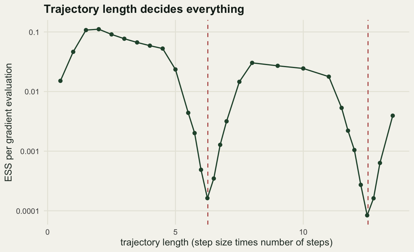
The vertical axis is logarithmic because a linear one would show a flat line with two invisible holes in it. The best trajectory length gives 0.1111 effective draws per gradient and the worst gives 8.383e-05, a factor of 1325.4 between two settings of one number.
Two things about that collapse deserve emphasis. First, the acceptance rate never warns you: the lowest acceptance anywhere in the sweep is 0.9871, so at the bottom of the dip the sampler is accepting almost every proposal and dutifully returning it to where it started. Any diagnostic built on acceptance is blind to this. Second, a well-tuned random-walk sampler on the same five-dimensional target gets 0.0558 effective draws per evaluation, which beats the badly tuned HMC by a factor of 665.9. A gradient-based sampler with the wrong trajectory length is far worse than no gradients at all.
This is the problem the No-U-Turn sampler solves, by extending each trajectory until it starts to double back on itself and stopping there, so the number of steps is chosen afresh at every iteration and never has to be guessed. That is why Stan does not ask you for a trajectory length.
What to take away
Hamiltonian Monte Carlo is four ideas stacked: minus the log posterior as a potential, a Gaussian momentum to push against it, the leapfrog to integrate the resulting dynamics, and a Metropolis accept step to absorb the integration error. The leapfrog earns its place by being exactly reversible and exactly volume preserving, measured here at 1.11e-15 and 8.148e-11. The accept step earns its place by producing a mean, a standard deviation and a correlation that sit about one Monte Carlo standard error from the closed form. Nothing in the method is mysterious once the pieces are separated.
What the measurements say about when to use it is more qualified than the usual story. On the two-parameter collinear posterior the gain over a well-tuned random walk was 3.0711 per evaluation, not an order of magnitude, and the random walk got there by accepting 0.0331 of proposals rather than the textbook 0.234. The gain grew with dimension, reaching 28.01 at 25 dimensions on a target with no correlation at all, which says the advantage is mostly about dimension rather than about geometry. And the whole case depends on cheap gradients: a finite-difference gradient costs 2 potential evaluations per dimension, and at every dimension tested that cost exceeds the measured gain, so the random walk wins.
The honest limit is that HMC needs a gradient of the log posterior everywhere, so discrete parameters have to be marginalised out by hand before the sampler ever sees the model, and the geometry it exploits belongs to the parameterisation you happened to write down rather than to the model, so the same posterior written two ways can be easy or impossible to sample. Two smaller caveats sit underneath that. Every target here is Gaussian, chosen so that each claim could be checked against a closed form, whereas a real hierarchical posterior has curvature that no single step size fits. And the effective sample size estimator caps at the chain length, so every HMC number reported is a floor. What to do about the parameterisation is the subject of the next post in this cluster.
References
Duane S, Kennedy AD, Pendleton BJ, Roweth D 1987 Physics Letters B 195(2):216-222 (10.1016/0370-2693(87)91197-X)
Hoffman MD, Gelman A 2014 Journal of Machine Learning Research 15:1593-1623
Betancourt M 2017 arXiv preprint (10.48550/arXiv.1701.02434)
Carpenter B, Gelman A, Hoffman MD, Lee D, Goodrich B, Betancourt M, Brubaker M, Guo J, Li P, Riddell A 2017 Journal of Statistical Software 76(1):1-32 (10.18637/jss.v076.i01)
Monnahan CC, Thorson JT, Branch TA 2017 Methods in Ecology and Evolution 8(3):339-348 (10.1111/2041-210X.12681)
Roberts GO, Gelman A, Gilks WR 1997 Annals of Applied Probability 7(1):110-120 (10.1214/aoap/1034625254)
Geyer CJ 1992 Statistical Science 7(4):473-483 (10.1214/ss/1177011137)