library(ggplot2)

te_pal <- list(forest = "#275139", green = "#2f8f63", sage = "#93a87f",
               clay = "#b5534e", gold = "#cda23f", line = "#dad9ca",
               ink = "#16241d", paper = "#f5f4ee")

theme_te <- function() {
  theme_minimal(base_size = 12) +
    theme(panel.grid.minor = element_blank(),
          panel.grid.major = element_line(colour = "#e7e6dc"),
          plot.background = element_rect(fill = "#f5f4ee", colour = NA),
          panel.background = element_rect(fill = "#f5f4ee", colour = NA),
          plot.title = element_text(face = "bold", colour = te_pal$ink),
          axis.title = element_text(colour = "#2c3a31"),
          legend.position = "bottom")
}Reparameterisation and Neal’s funnel
R
MCMC
Bayesian statistics
hierarchical models
ecology tutorial
Why hierarchical ecological models warn in Stan: measure the centred parameterisation failing on Neal’s funnel, fix it, and find where centred wins again.
The bat survey has twenty transects and several years of counts. Someone fits the obvious model: each transect gets its own activity offset, the offsets are drawn from a normal distribution whose standard deviation is estimated, and the counts follow from there. The model compiles. The chains run. Then the sampler prints a line that stops the analysis dead: there were divergent transitions after warmup, and the results may be biased.
The advice that follows is always the same. Increase adapt_delta. Reparameterise. Use a tighter prior. The first often does nothing except make the run slower, the second is offered without saying what it does, and the third changes the model when the analyst only wanted to change the arithmetic. Meanwhile the summary table looks reasonable: sensible point estimates, sensible interval widths, and nothing that says which of those numbers you should not believe.
The thing being warned about is geometry, not statistics. A hierarchical model contains a group-level standard deviation, and it contains group effects whose scale is that standard deviation. Written the natural way, those two sets of parameters are wound tightly around each other: the smaller the standard deviation gets, the narrower the region the group effects are allowed to occupy. The posterior is a funnel. Samplers that take steps of a fixed size cannot fit into the sharp end of it, so they stop short, and stopping short is invisible unless you know where the sharp end was supposed to be.
This post takes the smallest object with that geometry, a construction due to Radford Neal, and treats sampler failure as something to measure rather than something to warn about. The density is available in closed form, so the right answers are known before any chain is run. Everything is written in base R: a random walk Metropolis sampler, a Hamiltonian sampler with leapfrog integration, the divergence check that Stan reports, an effective sample size estimator and a split R-hat. The last section is the one the standard advice leaves out: the recommended fix is not always a fix, and the crossover point is measurable.
Four earlier posts set this one up. Hamiltonian Monte Carlo from scratch builds the gradient sampler that is used here without further comment, Bayesian hierarchical models with MCMC builds the ecological model whose geometry this is, MCMC convergence diagnostics builds R-hat and the effective sample size by hand, and Choosing priors: flat is not uninformative covers the prior on the group-level standard deviation, which is what controls how deep the neck goes.
A funnel whose answer is known in advance
Neal’s funnel strips a hierarchical model down to the part that causes the trouble. One parameter, called \(v\) here, is a log variance and has a normal prior. Nine further parameters, standing in for group effects, are normal with standard deviation \(\exp(v/2)\). There is no data and no likelihood. The density is a prior, and it is a prior that anybody who has written a hierarchical model has already written down without noticing.
Two facts make it the right test object. The joint density is available in closed form, so it can be drawn exactly rather than estimated. And the marginal distribution of \(v\) is exactly the normal prior it started with, because integrating out the nine coefficients returns their normalising constants and nothing else. The posterior mean of \(v\) is zero, its standard deviation is the prior standard deviation, and every quantile is a call to qnorm. Any disagreement between a chain and those numbers is a computational failure, not a modelling one.
n_coef <- 9
prior_sd <- 3

lp_centred <- function(pos) {
  v <- pos[1]; xs <- pos[-1]
  -v^2 / (2 * prior_sd^2) - n_coef * v / 2 - sum(xs^2) / (2 * exp(v))
}
gr_centred <- function(pos) {
  v <- pos[1]; xs <- pos[-1]
  c(-v / prior_sd^2 - n_coef / 2 + sum(xs^2) / (2 * exp(v)), -xs / exp(v))
}

lp_noncentred <- function(pos) {
  v <- pos[1]; zs <- pos[-1]
  -v^2 / (2 * prior_sd^2) - sum(zs^2) / 2
}
gr_noncentred <- function(pos) {
  v <- pos[1]; zs <- pos[-1]
  c(-v / prior_sd^2, -zs)
}

exact_q01 <- qnorm(0.01, 0, prior_sd); exact_q99 <- qnorm(0.99, 0, prior_sd)
print(round(c(coefficients = n_coef, prior_sd_of_v = prior_sd,
              exact_mean_v = 0, exact_sd_v = prior_sd,
              exact_q01 = exact_q01, exact_q99 = exact_q99,
              coef_sd_at_q01 = exp(exact_q01 / 2)), 4))
coefficients prior_sd_of_v exact_mean_v exact_sd_v exact_q01
9.0000 3.0000 0.0000 3.0000 -6.9790
exact_q99 coef_sd_at_q01
6.9790 0.0305 The two log densities above are the same model. lp_centred is the version an ecologist writes: the coefficients live on their natural scale and their spread is controlled by \(v\). lp_noncentred is the version after a change of variables, in which each coefficient is written as a standard normal deviate multiplied by \(\exp(v/2)\) and the sampler is handed the deviate instead. Sampling the second and multiplying afterwards gives draws from the first. That is the whole trick, and it is worth being precise about why it is not cheating.
A change of variables carries a Jacobian. Substituting \(x_j = z_j \exp(v/2)\) into the centred log density and adding the log Jacobian, which is \(n\,v/2\) for \(n\) coefficients, must give the non-centred log density back exactly, at every point, not approximately. That identity is checkable in two lines, so it should be checked rather than asserted.
set.seed(20260812)
probe <- matrix(rnorm(5 * (n_coef + 1)), 5)
gaps <- apply(probe, 1, function(row) {
  v <- 2 * row[1]
  zs <- row[-1]
  lp_noncentred(c(v, zs)) -
    (lp_centred(c(v, zs * exp(v / 2))) + n_coef * v / 2)
})
identity_gap <- max(abs(gaps))
gap_text <- format(signif(identity_gap, 3), scientific = TRUE)
print(c(probe_points = nrow(probe), max_abs_gap = gap_text))
probe_points max_abs_gap
"5" "3.55e-15" Across 5 random probe points the largest discrepancy is 3.55e-15, which is floating point noise. The two log densities describe one posterior. Anything that differs between them from here on is a property of the sampler and its coordinates, not of the model, the prior or the data.
The shape is worth stating plainly before any sampling happens. When \(v\) is large the coefficients have standard deviation \(\exp(v/2)\), which is large, so the density is wide. When \(v\) is small the coefficients are squeezed into a region of width \(\exp(v/2)\), which shrinks towards zero without ever reaching it. The result is a mouth and a neck. The neck has no bottom: the exact one per cent quantile of \(v\) is -6.979, and one draw in a hundred should be below it. At that depth the coefficients occupy a band of width 0.0305. A sampler that moves in steps of a fixed size in the coefficient directions cannot make a proposal that lands in a band that narrow.
Two samplers on the centred parameterisation
Both samplers are written out in full because the failure is in their mechanics. Random walk Metropolis proposes a normal jump around the current point and accepts on the density ratio. Hamiltonian Monte Carlo draws a momentum, integrates Hamilton’s equations with the leapfrog scheme for a fixed number of steps of a fixed size, and accepts on the change in total energy. The leapfrog integrator is where the divergence check lives, so it gets a gradient counter and a flag for trajectories whose energy error blows up.
rw_metropolis <- function(lp, start, n_iter, jump_sd) {
  n_par <- length(start)
  out <- matrix(0, n_iter, n_par)
  pos <- start; lp_now <- lp(pos); n_acc <- 0L
  for (i in seq_len(n_iter)) {
    prop <- pos + rnorm(n_par, 0, jump_sd)
    lp_prop <- lp(prop)
    if (log(runif(1)) < lp_prop - lp_now) {
      pos <- prop
      lp_now <- lp_prop
      n_acc <- n_acc + 1L
    }
    out[i, ] <- pos
  }
  list(draws = out, accept = n_acc / n_iter)
}

hmc <- function(lp, gr, start, n_iter, step, n_leap, d_max) {
  n_par <- length(start)
  out <- matrix(0, n_iter, n_par); divergent <- logical(n_iter)
  pos <- start; n_acc <- 0L; n_grad <- 0L
  for (i in seq_len(n_iter)) {
    mom <- rnorm(n_par)
    h_start <- -lp(pos) + sum(mom^2) / 2
    prop <- pos; mom_now <- mom
    gvec <- gr(prop); n_grad <- n_grad + 1L
    broke <- FALSE
    for (l in seq_len(n_leap)) {
      mom_now <- mom_now + 0.5 * step * gvec
      prop <- prop + step * mom_now
      gvec <- gr(prop)
      n_grad <- n_grad + 1L
      mom_now <- mom_now + 0.5 * step * gvec
      if (!all(is.finite(prop)) || !all(is.finite(gvec))) {
        broke <- TRUE
        break
      }
    }
    h_end <- if (broke) Inf else -lp(prop) + sum(mom_now^2) / 2
    if (!is.finite(h_end)) h_end <- Inf
    d_energy <- h_end - h_start
    divergent[i] <- (d_energy > d_max) || broke
    if (!divergent[i] && log(runif(1)) < -d_energy) {
      pos <- prop
      n_acc <- n_acc + 1L
    }
    out[i, ] <- pos
  }
  list(draws = out, accept = n_acc / n_iter,
       divergent = divergent, n_grad = n_grad)
}
Two diagnostics are needed as well. The effective sample size uses Geyer’s initial positive sequence: sum the autocorrelations in adjacent pairs, stop at the first pair that is not positive, and divide the chain length by the resulting integrated autocorrelation time. Split R-hat cuts each chain in half, treats the halves as separate chains, and compares the variance between chain means with the variance within chains.
ess_geyer <- function(x) {
  n <- length(x)
  if (var(x) < 1e-12) return(0)
  rho <- as.numeric(acf(x, lag.max = min(n - 1L, 400L), plot = FALSE)$acf)[-1]
  n_pair <- floor(length(rho) / 2)
  pairs <- rho[2 * (1:n_pair) - 1] + rho[2 * (1:n_pair)]
  first_bad <- which(pairs <= 0)[1]
  if (is.na(first_bad)) first_bad <- n_pair + 1L
  keep <- if (first_bad > 1L) pairs[1:(first_bad - 1L)] else 0
  tau_int <- 1 + 2 * sum(keep)
  min(n, n / max(tau_int, 1))
}

split_rhat <- function(chains) {
  n <- nrow(chains)
  half <- floor(n / 2)
  halves <- cbind(chains[1:half, , drop = FALSE],
                  chains[(n - half + 1):n, , drop = FALSE])
  within <- mean(apply(halves, 2, var))
  between <- half * var(colMeans(halves))
  sqrt((((half - 1) / half) * within + between / half) / within)
}
Now the runs. Four chains of two thousand iterations each for the Hamiltonian sampler, with twenty leapfrog steps per iteration and a step size of 0.4, which is close to what a step size adapter targeting an acceptance rate of 0.8 would choose here. The divergence threshold is the energy error that Stan uses. The random walk gets four chains of eight thousand iterations, because it needs them and because the density evaluations are cheap. Both samplers are run on both parameterisations from the same starting points.
n_chain <- 4; n_iter <- 2000
hmc_step <- 0.4; n_leap <- 20; d_max <- 1000

set.seed(20260729)
v_cen <- matrix(0, n_iter, n_chain); v_non <- matrix(0, n_iter, n_chain)
all_cen <- array(0, c(n_iter, n_chain, n_coef + 1))
x_cen <- NULL; x_non <- NULL; div_pts <- NULL
n_div_cen <- 0L; n_div_non <- 0L
acc_cen <- 0; acc_non <- 0
for (ch in seq_len(n_chain)) {
  start <- c(rnorm(1), rnorm(n_coef))
  fit_c <- hmc(lp_centred, gr_centred, start, n_iter, hmc_step, n_leap, d_max)
  fit_n <- hmc(lp_noncentred, gr_noncentred, start, n_iter, hmc_step, n_leap, d_max)
  all_cen[, ch, ] <- fit_c$draws
  v_cen[, ch] <- fit_c$draws[, 1]
  v_non[, ch] <- fit_n$draws[, 1]
  x_cen <- c(x_cen, fit_c$draws[, 2])
  x_non <- c(x_non, fit_n$draws[, 2] * exp(fit_n$draws[, 1] / 2))
  n_div_cen <- n_div_cen + sum(fit_c$divergent)
  n_div_non <- n_div_non + sum(fit_n$divergent)
  acc_cen <- acc_cen + fit_c$accept / n_chain
  acc_non <- acc_non + fit_n$accept / n_chain
  div_pts <- rbind(div_pts, fit_c$draws[fit_c$divergent, 1:2, drop = FALSE])
}
n_draw <- n_iter * n_chain
exact_min <- qnorm(1 / (n_draw + 1), 0, prior_sd)
print(round(c(chains = n_chain, iterations_each = n_iter, draws_total = n_draw,
              leapfrog_steps = n_leap, step_size = hmc_step,
              accept_centred = acc_cen, accept_noncentred = acc_non), 4))
chains iterations_each draws_total leapfrog_steps
4.0000 2000.0000 8000.0000 20.0000
step_size accept_centred accept_noncentred
0.4000 0.7970 0.9518 n_rw <- 8000; rw_step <- 0.6
set.seed(20260730)
rw_cen <- matrix(0, n_rw, n_chain); rw_non <- matrix(0, n_rw, n_chain)
acc_rw_cen <- 0; acc_rw_non <- 0
for (ch in seq_len(n_chain)) {
start <- c(rnorm(1), rnorm(n_coef))
fit_c <- rw_metropolis(lp_centred, start, n_rw, rw_step)
fit_n <- rw_metropolis(lp_noncentred, start, n_rw, rw_step)
rw_cen[, ch] <- fit_c$draws[, 1]
rw_non[, ch] <- fit_n$draws[, 1]
acc_rw_cen <- acc_rw_cen + fit_c$accept / n_chain
acc_rw_non <- acc_rw_non + fit_n$accept / n_chain
}
print(round(c(rw_iterations_each = n_rw, rw_draws_total = n_rw * n_chain,
rw_jump_sd = rw_step,
accept_centred = acc_rw_cen, accept_noncentred = acc_rw_non), 4))rw_iterations_each rw_draws_total rw_jump_sd accept_centred
8.000e+03 3.200e+04 6.000e-01 2.848e-01
accept_noncentred
3.963e-01 The Hamiltonian chains accepted 0.797 of proposals on the centred parameterisation and 0.9518 on the non-centred one, and the random walk accepted 0.2848 and 0.3963. Those are the numbers an analyst usually looks at first, and all four of them are fine. Now the same four chains get compared against the exact answer.
summarise_v <- function(chains, label) {
  data.frame(sampler = label,
             mean_v = mean(chains),
             sd_v = sd(chains),
             min_v = min(chains),
             frac_below_q01 = mean(chains < exact_q01),
             ess_v = sum(apply(chains, 2, ess_geyer)),
             rhat_v = split_rhat(chains))
}
failure <- rbind(summarise_v(rw_cen, "rw centred"),
                 summarise_v(rw_non, "rw non-centred"),
                 summarise_v(v_cen, "hmc centred"),
                 summarise_v(v_non, "hmc non-centred"))
failure[, -1] <- round(failure[, -1], 4)
print(failure)
sampler mean_v sd_v min_v frac_below_q01 ess_v rhat_v
1 rw centred -0.0258 1.8209 -3.3191 0.0000 74.5629 1.1111
2 rw non-centred -0.1165 3.0295 -11.1353 0.0129 147.0989 1.0228
3 hmc centred 1.1992 2.2458 -3.0352 0.0000 109.9008 1.0338
4 hmc non-centred -0.0120 3.0101 -12.1507 0.0099 8000.0000 0.9995print(round(c(exact_mean = 0, exact_sd = prior_sd, exact_frac_below_q01 = 0.01,
expected_min_of_n_draws = exact_min), 4)) exact_mean exact_sd exact_frac_below_q01
0.0000 3.0000 0.0100
expected_min_of_n_draws
-10.9869 Read the table one column at a time. The exact posterior mean of \(v\) is zero; the centred Hamiltonian chains return 1.1992 and the centred random walk returns -0.0258. The exact standard deviation is 3; the centred Hamiltonian chains return 2.2458 and the centred random walk 1.8209. Both centred runs understate the spread of the group-level variance, and neither of them is close. On the non-centred parameterisation the same two samplers return 3.0101 and 3.0295, both of which sit within one per cent of the truth.
The neck columns are worse than the moment columns. One per cent of the posterior mass sits below -6.979. Both centred runs put 0 of their draws there, visiting the tail not once in 8000 Hamiltonian draws or 32000 random walk draws. The deepest point the centred Hamiltonian sampler reached in 8000 draws is -3.0352; with independent draws from the exact marginal, the expected minimum of that many is -10.9869. The chain stopped a long way short of that, while accepting 0.797 of its proposals.
The effective sample sizes are the last column worth stopping on. The non-centred Hamiltonian chains return 8000 effective draws from 8000, which is the cap: the draws of \(v\) are effectively independent. The centred chains return 109.9, a factor of 72.7929 worse from a change of variables that leaves the posterior identical to fifteen decimal places.
trace_df <- rbind(
  data.frame(iteration = seq_len(n_iter), v = v_cen[, 1], which = "centred"),
  data.frame(iteration = seq_len(n_iter), v = v_non[, 1], which = "non-centred"))
ggplot(trace_df, aes(iteration, v)) +
  geom_hline(yintercept = c(exact_q01, exact_q99), colour = te_pal$clay,
             linetype = "dashed", linewidth = 0.4) +
  geom_line(aes(colour = which), linewidth = 0.3) +
  facet_wrap(~which, ncol = 1) +
  scale_colour_manual(values = c(centred = te_pal$forest,
                                 `non-centred` = te_pal$green), guide = "none") +
  labs(x = "iteration", y = "log variance v",
       title = "Trace of v, exact 1 and 99 per cent quantiles dashed") +
  theme_te()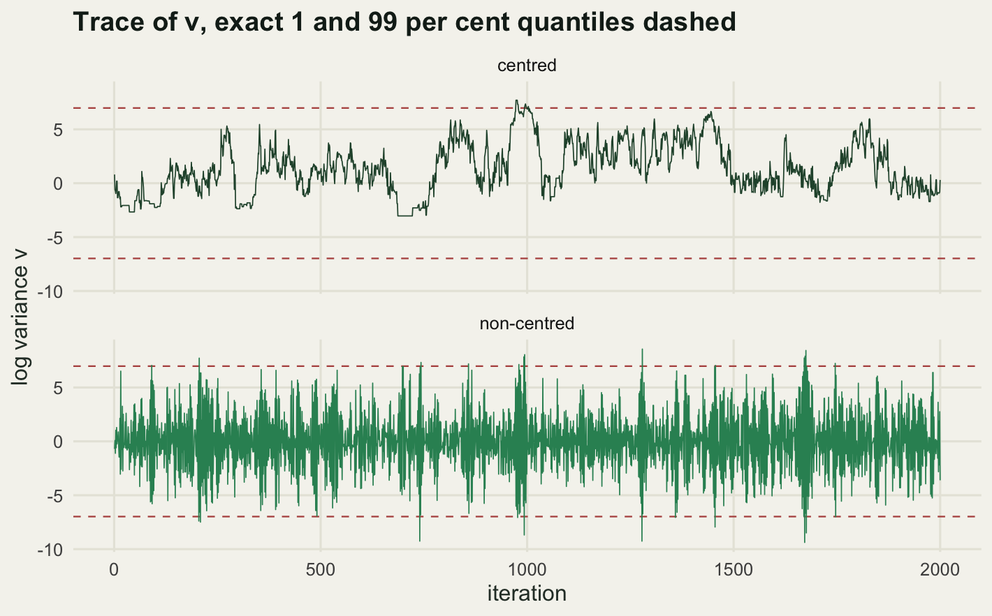
The trace makes the asymmetry of the failure visible in a way the table cannot. Both chains reach the upper dashed line, because the mouth of the funnel is wide and easy to move around in. Only one of them reaches the lower dashed line. The centred chain is not stuck in the usual sense: it moves and it explores. It simply has a floor under it that is not part of the model, and that floor sits at -3.0352 rather than at minus infinity.
An ecologist reading this off a real fit would conclude that the between-transect standard deviation is bounded away from zero. That conclusion would be an artefact of the step size.
What the diagnostics do and do not say
The centred run is wrong. The question is what a routine check would have said about it. A hierarchical fit puts two numbers on the screen for every parameter, an R-hat and an effective sample size. Here that is one scale parameter and 9 coefficients.
rhat_all <- apply(all_cen, 3, split_rhat)
ess_all <- apply(all_cen, 3, function(m) sum(apply(m, 2, ess_geyer)))
per_par <- data.frame(parameter = c("v", paste0("x", seq_len(n_coef))),
                      rhat = round(rhat_all, 4),
                      ess = round(ess_all, 1))
print(per_par)
parameter rhat ess
1 v 1.0338 109.9
2 x1 1.0071 898.2
3 x2 1.0054 586.8
4 x3 1.0071 756.1
5 x4 1.0151 380.2
6 x5 1.0071 836.5
7 x6 1.0306 347.0
8 x7 1.0019 570.0
9 x8 1.0053 787.2
10 x9 1.0110 352.6print(round(c(conventional_rhat_threshold = 1.01,
best_coefficient_rhat = min(rhat_all[-1]),
worst_coefficient_rhat = max(rhat_all[-1]),
worst_coefficient_ess = min(ess_all[-1]),
rhat_of_v = rhat_all[1], ess_of_v = ess_all[1],
ess_ratio_worst_coef_to_v = min(ess_all[-1]) / ess_all[1],
sd_error_centred = prior_sd - failure$sd_v[3],
divergence_rate_centred = n_div_cen / n_draw,
divergence_rate_noncentred = n_div_non / n_draw), 5))conventional_rhat_threshold best_coefficient_rhat
1.01000 1.00189
worst_coefficient_rhat worst_coefficient_ess
1.03058 346.96214
rhat_of_v ess_of_v
1.03379 109.90079
ess_ratio_worst_coef_to_v sd_error_centred
3.15705 0.75420
divergence_rate_centred divergence_rate_noncentred
0.00325 0.00000 R-hat is not silent here, and it would be convenient for the story if it were. The R-hat for \(v\) is 1.0338, well above the conventional threshold of 1.01. The 9 coefficients run from 1.0019 to 1.0306, so on a strict reading several of them are over the line as well. That is the diagnostic doing its job rather than a false alarm: the coefficients take their scale from \(v\), so chains that disagree about \(v\) disagree a little about the coefficients too.
Two things are still wrong with signing the fit off on those numbers. The first is the size of the complaint against the size of the error. An R-hat of 1.0338 is the sort of number that gets a model rerun with more iterations and no further thought, and what it is reporting is a posterior standard deviation that is out by 0.7542 on a true value of 3. The effective sample sizes separate the parameters more usefully: 109.9 for \(v\) against 347 for the worst coefficient, a ratio of 3.15705.
The second is that more iterations will not help. R-hat measures disagreement between chains, and this failure is shared: all four chains have the same floor at -3.0352, put there by the step size and the geometry rather than by the chain length. What R-hat picks up is the leftover variation in how far each chain wandered above that floor, and running longer shrinks that leftover variation without moving the floor. Neither R-hat nor the effective sample size says where the trouble is or which way the bias runs.
The divergence rate is a different kind of instrument, because it points at a location rather than at a number. The centred run flagged 0.00325 of its transitions as divergent; the non-centred run flagged none at all, a rate of 0.
Divergences, and how easily they go quiet
A divergent transition is not a failed proposal. The leapfrog integrator conserves total energy approximately, and the approximation is good as long as the step size is small relative to the curvature of the log density. In the neck of the funnel the curvature in the coefficient directions grows without bound, the integrator is no longer approximately symplectic, and the trajectory picks up an energy error of a size that could not happen by chance. Flagging that error is the only warning available, because the sampler cannot tell from inside the mouth that a neck exists.
div_summary <- c(n_divergent = nrow(div_pts),
                 median_v_at_divergence = median(div_pts[, 1]),
                 max_v_at_divergence = max(div_pts[, 1]),
                 median_v_all_draws = median(v_cen),
                 frac_divergences_below_median = mean(div_pts[, 1] < median(v_cen)))
print(round(div_summary, 4))
n_divergent median_v_at_divergence
26.0000 -2.1208
max_v_at_divergence median_v_all_draws
-0.0151 0.8747
frac_divergences_below_median
1.0000 All 26 divergent transitions in the centred run started below the median of the chain. Not most of them: all of them, a fraction of 1. The median \(v\) at a divergence is -2.1208 against a median of 0.8747 over all draws, and the highest \(v\) at which any divergence occurred is -0.0151. The divergences are not scattered noise. They mark the exact region the sampler was trying to enter and could not.
div_plot <- rbind(
  data.frame(v = as.vector(v_cen), x = x_cen, kind = "all draws"),
  data.frame(v = div_pts[, 1], x = div_pts[, 2], kind = "divergent"))
ggplot(div_plot, aes(v, x, colour = kind, size = kind, alpha = kind)) +
  geom_point() +
  scale_colour_manual(values = c(`all draws` = te_pal$sage,
                                 divergent = te_pal$clay), name = NULL) +
  scale_size_manual(values = c(`all draws` = 0.6, divergent = 1.5), name = NULL) +
  scale_alpha_manual(values = c(`all draws` = 0.4, divergent = 1), name = NULL) +
  labs(x = "log variance v", y = "first coefficient x1",
       title = "Divergences sit at the deepest point the chain reached") +
  theme_te()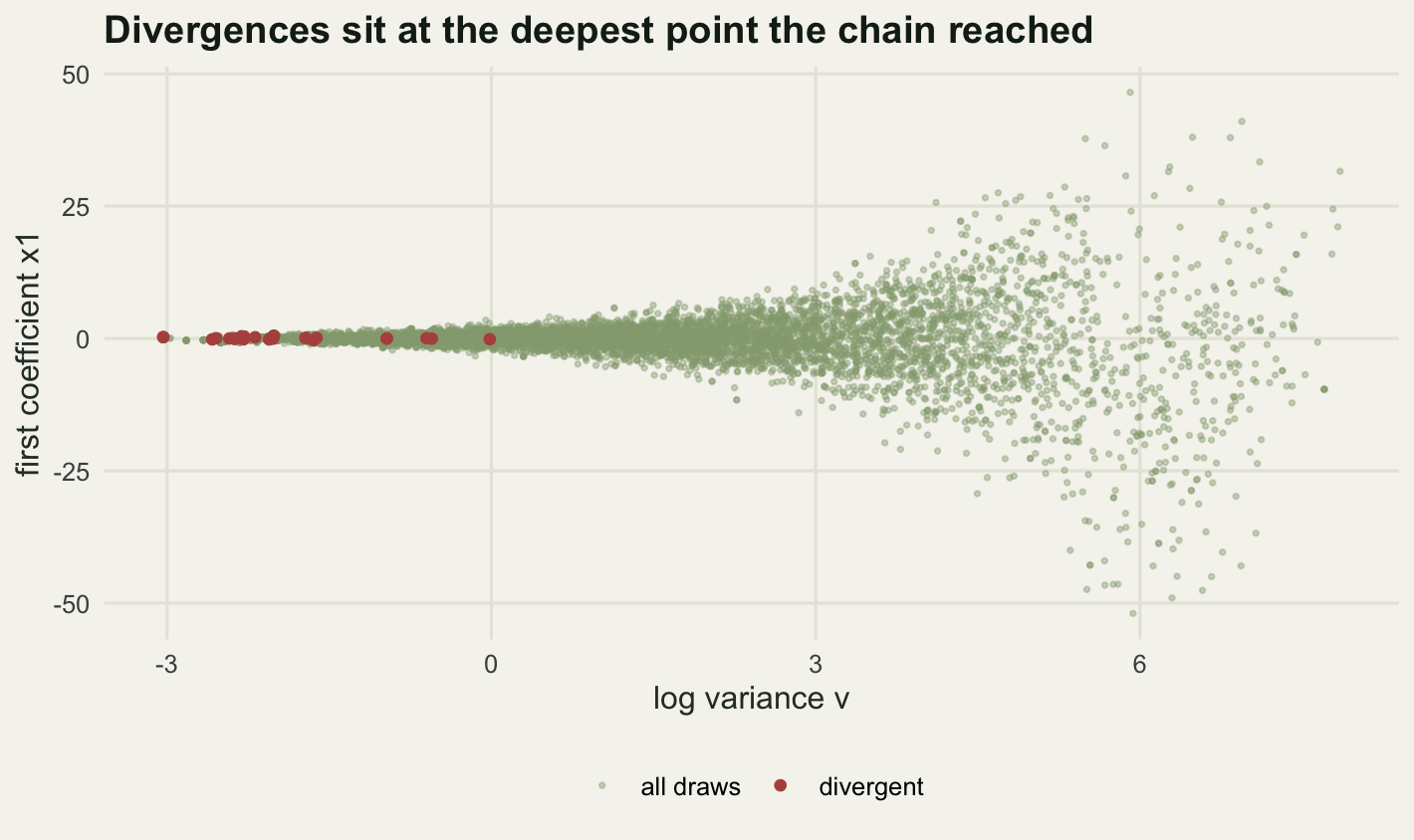
That picture is the argument for taking divergences seriously, and also for not trusting their absence. The usual response to a divergence warning is to reduce the step size, which is what raising adapt_delta does, so the whole experiment is repeated at five step sizes with a fresh set of four chains at each.
step_grid <- c(0.15, 0.2, 0.3, 0.4, 0.6)
sweep_rows <- NULL
for (this_step in step_grid) {
  set.seed(20260731)
  vs <- matrix(0, n_iter, n_chain); n_div <- 0L; acc <- 0
  for (ch in seq_len(n_chain)) {
    start <- c(rnorm(1), rnorm(n_coef))
    fit_c <- hmc(lp_centred, gr_centred, start, n_iter, this_step, n_leap, d_max)
    vs[, ch] <- fit_c$draws[, 1]
    n_div <- n_div + sum(fit_c$divergent)
    acc <- acc + fit_c$accept / n_chain
  }
  sweep_rows <- rbind(sweep_rows,
                      data.frame(step = this_step, accept = acc,
                                 div_n = n_div, div_rate = n_div / n_draw,
                                 sd_v = sd(vs), min_v = min(vs),
                                 ess_v = sum(apply(vs, 2, ess_geyer)),
                                 rhat_v = split_rhat(vs)))
}
print(round(sweep_rows, 4))
step accept div_n div_rate sd_v min_v ess_v rhat_v
1 0.15 0.9220 1 0.0001 2.7111 -5.0720 106.2475 1.0654
2 0.20 0.8521 12 0.0015 2.7636 -4.4940 54.3331 1.1670
3 0.30 0.8419 13 0.0016 2.3060 -3.4253 120.8977 1.0253
4 0.40 0.7306 128 0.0160 2.3944 -3.0520 83.5905 1.1007
5 0.60 0.3136 1794 0.2242 2.0622 -1.8841 43.7647 1.1915sweep_gain <- c(pct_of_sd_error_removed =
100 * (sweep_rows$sd_v[1] - sweep_rows$sd_v[5]) / (prior_sd - sweep_rows$sd_v[5]))
print(round(sweep_gain, 4))pct_of_sd_error_removed
69.1916 This is the result that should change how the warning is read. At a step size of 0.6 the divergence rate is 0.2242, and any sampler would shout about it. At a step size of 0.15 the divergence rate is 0.0001, with 1 of the 8000 transitions flagged, at an acceptance rate of 0.922. That is the kind of number an analyst waves through. The warning has all but gone. The bias has not. The estimated standard deviation of \(v\) moves from 2.0622 at the largest step to 2.7111 at the smallest, against an exact value of 3. Going from a step of 0.6 to a step of 0.15 took the divergence count from 1794 to 1, and removed 69.1916 per cent of the error.
The deepest point reached tells the same story from the other side. It improves from -1.8841 to -5.072 as the step shrinks, which is real progress, and it is still nowhere near the -10.9869 that 8000 independent draws would have produced. A smaller step lets the chain slide further into the neck before the integrator breaks, and the break stops producing an energy error large enough to trip the threshold. A quiet divergence counter is evidence that the step size is small, not that the answer is right.
The last two columns of the sweep are worth reading together. The effective sample size bounces from 54.3331 to 106.2475 with no clean trend, because four chains of 2000 iterations is not enough to pin down a number of that order. The R-hat for \(v\) runs from 1.0253 to 1.1915 and is likewise unrelated to the step size. Both complain at every setting, and neither points at the setting as the thing to change. The divergence rate and the depth reached are the columns carrying information here.
The fix, and what it is worth
The non-centred parameterisation replaces each coefficient \(x_j\) with \(z_j \exp(v/2)\) and hands the sampler \(z_j\). The posterior in the new coordinates is the product of a normal for \(v\) and nine independent standard normals, which is why lp_noncentred has no interaction term at all. There is no neck, because the width of the \(z\) directions no longer depends on \(v\), and a fixed step size is exactly the right tool for a target like that.
improve <- c(ess_factor = failure$ess_v[4] / failure$ess_v[3],
             sd_error_centred = abs(failure$sd_v[3] - prior_sd),
             sd_error_noncentred = abs(failure$sd_v[4] - prior_sd),
             mean_error_centred = abs(failure$mean_v[3]),
             mean_error_noncentred = abs(failure$mean_v[4]),
             depth_centred = failure$min_v[3], depth_noncentred = failure$min_v[4],
             depth_expected = exact_min, tail_centred = failure$frac_below_q01[3],
             tail_noncentred = failure$frac_below_q01[4], tail_exact = 0.01)
print(round(improve, 4))
ess_factor sd_error_centred sd_error_noncentred
72.7929 0.7542 0.0101
mean_error_centred mean_error_noncentred depth_centred
1.1992 0.0120 -3.0352
depth_noncentred depth_expected tail_centred
-12.1507 -10.9869 0.0000
tail_noncentred tail_exact
0.0099 0.0100 Every column moves in the same direction and most of them move by a lot. The error in the posterior standard deviation of \(v\) falls from 0.7542 to 0.0101. The error in the posterior mean falls from 1.1992 to 0.012. The fraction of draws in the lower one per cent tail goes from 0 to 0.0099, against the exact 0.01. The deepest point reached goes from -3.0352 to -12.1507, against -10.9869 for independent draws. And the effective sample size for \(v\) improves by a factor of 72.7929 at identical cost per iteration, since both parameterisations use the same number of leapfrog steps and the gradients cost the same.
grid_v <- seq(-13, 11, length.out = 240); grid_u <- seq(-6, 6, length.out = 300)
dens <- expand.grid(v = grid_v, u = grid_u)
dens$ld <- -dens$v^2 / (2 * prior_sd^2) - dens$v / 2 -
  sinh(dens$u)^2 / (2 * exp(dens$v))
dens$ld <- dens$ld - max(dens$ld)
dens2 <- rbind(cbind(dens, which = "centred"), cbind(dens, which = "non-centred"))
clouds <- rbind(
  data.frame(v = as.vector(v_cen), u = asinh(x_cen), which = "centred"),
  data.frame(v = as.vector(v_non), u = asinh(x_non), which = "non-centred"))
clouds$kind <- ifelse(clouds$v < exact_q01, "below the 1 per cent quantile", "draw")
n_deep <- table(clouds$which, clouds$kind)[, 1]
ggplot() +
  geom_vline(xintercept = exact_q01, colour = te_pal$gold,
             linetype = "dashed", linewidth = 0.5) +
  geom_point(data = clouds, aes(v, u, colour = kind, size = kind, alpha = kind)) +
  geom_contour(data = dens2, aes(v, u, z = ld), breaks = c(-2, -5, -10, -18),
               colour = te_pal$ink, linewidth = 0.3) +
  facet_wrap(~which) +
  scale_colour_manual(values = c(draw = te_pal$sage,
                                 `below the 1 per cent quantile` = te_pal$clay),
                      name = NULL) +
  scale_size_manual(values = c(draw = 0.55,
                               `below the 1 per cent quantile` = 1.3), name = NULL) +
  scale_alpha_manual(values = c(draw = 0.3,
                                `below the 1 per cent quantile` = 1), name = NULL) +
  scale_y_continuous(breaks = asinh(c(-30, -3, 0, 3, 30)),
                     labels = c(-30, -3, 0, 3, 30)) +
  coord_cartesian(xlim = c(-11.5, 7.5), ylim = c(-4.2, 4.2)) +
  labs(x = "log variance v", y = "first coefficient x1 (axis stretched near zero)",
       title = "Exact funnel contours with each sampler's draws") +
  theme_te()
print(n_deep)
centred non-centred
0 79 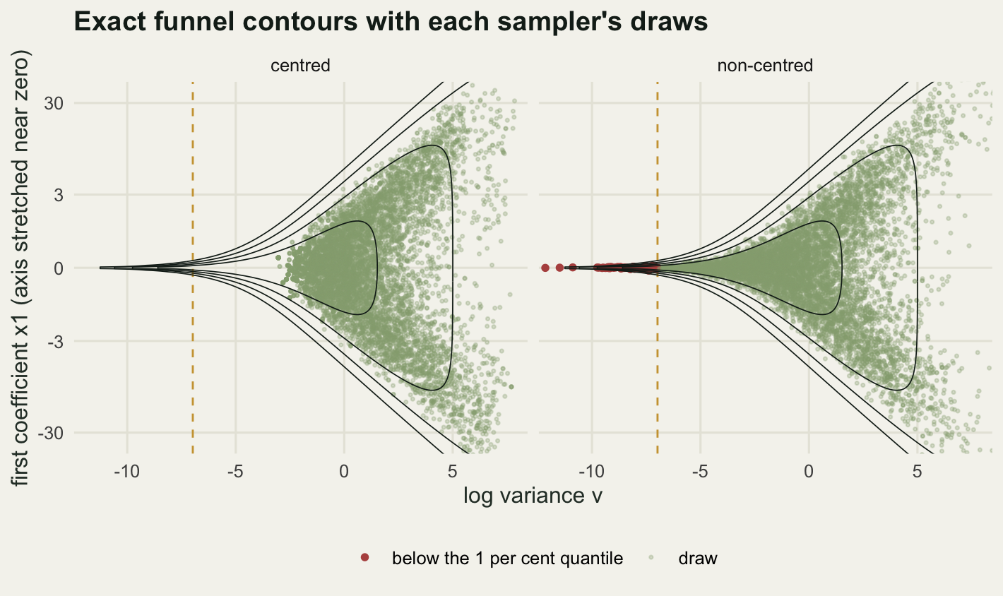
The vertical axis is stretched near zero, using an inverse hyperbolic sine scale, because otherwise the neck collapses onto a single row of pixels and the difference between the panels disappears. The contour lines are the exact log density, computed on a grid rather than estimated from the draws. Both clouds fill the mouth identically, which is the point: the failure is not visible anywhere a routine posterior predictive check would look. It is visible only left of the gold line, where the non-centred run placed 79 draws and the centred run placed 0.
At this stage the standard advice looks vindicated, and most treatments stop here. The next section is the reason they should not.
When the centred version is the better one
The funnel has no data in it. A real hierarchical model does, and the likelihood pulls the group effects towards their own group means, which changes the geometry. With many observations per group, each group effect is pinned down by its own data almost independently of the group-level standard deviation, and the funnel flattens out. In the non-centred coordinates the opposite happens: the sampler is working with \(z_j\), and the data constrain \(z_j \exp(v)\) rather than \(z_j\), so the likelihood introduces exactly the kind of dependence between \(v\) and the coefficients that the reparameterisation was meant to remove.
The model for this section is a normal hierarchy: twenty groups, a group-level standard deviation with a lognormal prior, and a group mean estimated from a number of observations per group that will be swept from one to sixty-four. The residual standard deviation is fixed at one, and the likelihood goes through the group means because the within-group scatter is a constant. Both parameterisations are written out, with the Jacobian folded in as before.
n_grp <- 20; tau_true <- 0.25

hlp_centred <- function(pos, ybar, n_obs) {
  v <- pos[1]; eff <- pos[-1]
  -v^2 / 2 - n_grp * v - sum(eff^2) / (2 * exp(2 * v)) -
    n_obs * sum((ybar - eff)^2) / 2
}
hgr_centred <- function(pos, ybar, n_obs) {
  v <- pos[1]; eff <- pos[-1]
  c(-v - n_grp + sum(eff^2) / exp(2 * v),
    -eff / exp(2 * v) + n_obs * (ybar - eff))
}

hlp_noncentred <- function(pos, ybar, n_obs) {
  v <- pos[1]; zs <- pos[-1]
  -v^2 / 2 - sum(zs^2) / 2 - n_obs * sum((ybar - zs * exp(v))^2) / 2
}
hgr_noncentred <- function(pos, ybar, n_obs) {
  v <- pos[1]; zs <- pos[-1]
  resid <- n_obs * (ybar - zs * exp(v))
  c(-v + sum(resid * zs) * exp(v), -zs + resid * exp(v))
}
print(round(c(groups = n_grp, true_group_sd = tau_true,
              residual_sd = 1), 4))
groups true_group_sd residual_sd
20.00 0.25 1.00 Comparing two samplers fairly needs a step size for each chosen the same way, and a cost measure that is not a clock. The step size comes from dual averaging during a warmup phase, targeting an acceptance probability of 0.8, which is what Stan does. The cost is the number of gradient evaluations during the sampling phase, counted exactly by the sampler. The reported quantity is effective draws of \(v\) per thousand gradients: a sampler that mixes twice as well while doing three times the work is not a better sampler.
hmc_adapt <- function(lp, gr, start, n_warm, n_samp, n_leap, target = 0.8) {
  n_par <- length(start)
  pos <- start; step <- 0.2; anchor <- log(10 * step)
  h_bar <- 0; log_step_bar <- 0; n_grad <- 0L
  out <- matrix(0, n_samp, n_par)
  one_step <- function(pos, step) {
    mom <- rnorm(n_par)
    h_start <- -lp(pos) + sum(mom^2) / 2
    prop <- pos; mom_now <- mom
    gvec <- gr(prop); used <- 1L
    broke <- FALSE
    for (l in seq_len(n_leap)) {
      mom_now <- mom_now + 0.5 * step * gvec
      prop <- prop + step * mom_now
      gvec <- gr(prop)
      used <- used + 1L
      mom_now <- mom_now + 0.5 * step * gvec
      if (!all(is.finite(prop)) || !all(is.finite(gvec))) {
        broke <- TRUE
        break
      }
    }
    h_end <- if (broke) Inf else -lp(prop) + sum(mom_now^2) / 2
    if (!is.finite(h_end)) h_end <- Inf
    d_energy <- h_end - h_start
    alpha <- if (d_energy > 700) 0 else min(1, exp(-d_energy))
    bad <- (d_energy > 1000) || broke
    keep <- (!bad) && (log(runif(1)) < -d_energy)
    list(pos = if (keep) prop else pos, alpha = alpha, used = used)
  }
  for (m in seq_len(n_warm)) {
    got <- one_step(pos, step)
    pos <- got$pos
    h_bar <- (1 - 1 / (m + 10)) * h_bar + (1 / (m + 10)) * (target - got$alpha)
    log_step <- anchor - sqrt(m) / 0.05 * h_bar
    log_step_bar <- m^(-0.75) * log_step + (1 - m^(-0.75)) * log_step_bar
    step <- exp(log_step)
  }
  step <- exp(log_step_bar)
  for (m in seq_len(n_samp)) {
    got <- one_step(pos, step)
    pos <- got$pos
    n_grad <- n_grad + got$used
    out[m, ] <- pos
  }
  list(draws = out, step = step, n_grad = n_grad)
}
The sweep runs both parameterisations on four independently simulated data sets at each of seven group sizes. The group effects and the standardised noise are drawn once and reused across group sizes, so that increasing the number of observations per group changes only the precision of the group means and nothing else. Warmup is three hundred iterations, the sampling phase is eight hundred, and each trajectory uses twelve leapfrog steps, which keeps the whole sweep inside the runtime budget for the post.
obs_grid <- c(1, 2, 4, 8, 16, 32, 64)
n_rep <- 4
n_warm <- 300
n_samp <- 800
n_leap_sw <- 12

set.seed(20260805)
eff_true <- matrix(rnorm(n_rep * n_grp, 0, tau_true), n_rep, n_grp)
noise <- matrix(rnorm(n_rep * n_grp), n_rep, n_grp)

cross <- NULL
for (n_obs in obs_grid) {
  per_c <- numeric(n_rep); per_n <- numeric(n_rep)
  post_c <- numeric(n_rep); post_n <- numeric(n_rep)
  for (r in seq_len(n_rep)) {
    ybar <- eff_true[r, ] + noise[r, ] / sqrt(n_obs)
    set.seed(20260806 + r)
    fit_c <- hmc_adapt(function(pos) hlp_centred(pos, ybar, n_obs),
                       function(pos) hgr_centred(pos, ybar, n_obs),
                       c(log(tau_true), ybar), n_warm, n_samp, n_leap_sw)
    set.seed(20260806 + r)
    fit_n <- hmc_adapt(function(pos) hlp_noncentred(pos, ybar, n_obs),
                       function(pos) hgr_noncentred(pos, ybar, n_obs),
                       c(log(tau_true), ybar / tau_true), n_warm, n_samp, n_leap_sw)
    per_c[r] <- 1000 * ess_geyer(fit_c$draws[, 1]) / fit_c$n_grad
    per_n[r] <- 1000 * ess_geyer(fit_n$draws[, 1]) / fit_n$n_grad
    post_c[r] <- mean(fit_c$draws[, 1])
    post_n[r] <- mean(fit_n$draws[, 1])
  }
  cross <- rbind(cross, data.frame(obs_per_group = n_obs,
                                   centred = mean(per_c),
                                   noncentred = mean(per_n),
                                   ratio = mean(per_c) / mean(per_n),
                                   mean_v_centred = mean(post_c),
                                   mean_v_noncentred = mean(post_n)))
}
print(round(cross, 4))
obs_per_group centred noncentred ratio mean_v_centred mean_v_noncentred
1 1 2.2272 11.6446 0.1913 -0.8807 -0.8013
2 2 3.4527 10.6680 0.3236 -1.0678 -1.0286
3 4 9.0940 12.6657 0.7180 -1.2311 -1.2238
4 8 24.4488 7.4801 3.2685 -1.3429 -1.3435
5 16 22.2983 8.6805 2.5688 -1.4460 -1.3994
6 32 44.0854 8.9121 4.9467 -1.4530 -1.4103
7 64 76.4269 10.4527 7.3117 -1.4003 -1.3872log_ratio <- log(cross$ratio)
log_obs <- log(cross$obs_per_group)
first_win <- which(log_ratio > 0)[1]
crossover <- exp(log_obs[first_win - 1] +
(0 - log_ratio[first_win - 1]) / (log_ratio[first_win] - log_ratio[first_win - 1]) *
(log_obs[first_win] - log_obs[first_win - 1]))
print(round(c(group_sizes = length(obs_grid), replicates_per_size = n_rep,
warmup = n_warm, sampling = n_samp, leapfrog_steps = n_leap_sw,
target_accept = 0.8, crossover_obs_per_group = crossover), 4)) group_sizes replicates_per_size warmup
7.0000 4.0000 300.0000
sampling leapfrog_steps target_accept
800.0000 12.0000 0.8000
crossover_obs_per_group
4.6544 cross_gain <- c(centred_gain_over_sweep = cross$centred[7] / cross$centred[1],
max_mean_v_gap = max(abs(cross$mean_v_centred - cross$mean_v_noncentred)))
print(round(cross_gain, 4))centred_gain_over_sweep max_mean_v_gap
34.3148 0.0794 The two columns cross. At one observation per group the non-centred parameterisation returns 11.6446 effective draws per thousand gradients and the centred one returns 2.2272, so the centred form manages only a ratio 0.1913 of the non-centred rate. At sixty-four observations per group the centred parameterisation returns 76.4269 and the non-centred one returns 10.4527, so centred is better by a factor of 7.3117. Interpolating on the log scale, the two are equal at 4.654 observations per group.
The size of the swing matters as much as its direction. Across the sweep the centred parameterisation improves by a factor of 34.3148, while the non-centred one wanders between 7.5 and 12.7 with no trend and ends below where it started, at 10.4527. Using the non-centred version on the largest data set costs a factor of 7.3117, for a model where the natural parameterisation would have worked without any warning at all.
cross_long <- rbind(
  data.frame(lg = log2(cross$obs_per_group), y = cross$centred, which = "centred"),
  data.frame(lg = log2(cross$obs_per_group), y = cross$noncentred, which = "non-centred"))
ggplot(cross_long, aes(lg, y, colour = which, shape = which)) +
  geom_vline(xintercept = log2(crossover), colour = te_pal$ink,
             linetype = "dotted", linewidth = 0.5) +
  geom_line(linewidth = 0.7) +
  geom_point(size = 2.2) +
  scale_x_continuous(breaks = 0:6, labels = 2^(0:6)) +
  scale_colour_manual(values = c(centred = te_pal$clay,
                                 `non-centred` = te_pal$green), name = NULL) +
  scale_shape_manual(values = c(centred = 16, `non-centred` = 17), name = NULL) +
  labs(x = "observations per group",
       y = "effective draws per 1000 gradients",
       title = "Centred overtakes non-centred as the data sharpen") +
  theme_te()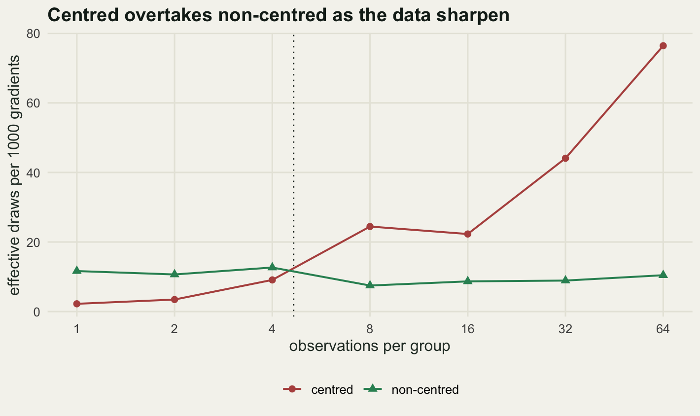
The mechanism behind the crossing is the one that produced the funnel, running backwards. In the centred coordinates the prior creates the dependence between \(v\) and the group effects and the likelihood breaks it, so more data per group means a flatter, easier posterior. In the non-centred coordinates the prior creates independence and the likelihood creates the dependence, so more data per group means a harder posterior. Which side wins depends on whether the prior or the likelihood is doing more work on the group effects, roughly the group-level variance against the sampling variance of a group mean. The crossover measured here, 4.654 observations per group, is in that region for a group-level standard deviation of 0.25 and a residual standard deviation of 1.
A check that both runs describe the same posterior sits in the last two columns. At the largest group size the posterior mean of \(v\) is -1.4003 from the centred runs and -1.3872 from the non-centred ones, which agree to within Monte Carlo error even though one needed several times as many gradients per effective draw. The disagreement across the sweep never exceeds 0.0794, and the largest gaps are at the small group sizes where the centred sampler is doing worst.
The practical reading is that neither parameterisation is the default. A study with two visits per transect and a weak between-transect signal belongs in the non-centred form. A study with sixty-four quadrats per site and real between-site variation belongs in the centred form, and switching it out of habit costs a factor of 7.3117. Mixed designs, where some groups have many observations and some few, belong in neither, which is why the newer samplers offer a per-group choice.
What to take away
Two ways of writing the same hierarchical model produced posterior standard deviations of 2.2458 and 3.0101 for a quantity whose exact value is 3, using the same sampler, the same step size, the same number of gradient evaluations and a change of variables that alters the log density by an amount no larger than 3.55e-15. The failing version accepted 0.797 of its proposals, and its summary table reported an R-hat of 1.0338 for \(v\). A number that mild does not convey an error that large, and nothing in the output says which way the error runs.
The divergence check is the one diagnostic that points at the problem rather than around it, and the step size sweep shows how to make it lie. Going from a step of 0.6 to a step of 0.15 took the divergence rate from 0.2242 to 0.0001, a fall from 1794 flagged transitions to 1, and the acceptance rate up to 0.922, while the estimated standard deviation of \(v\) moved from 2.0622 to 2.7111, still short of the exact 3. Turning up adapt_delta until the warnings stop is not the same as fixing the model, and the absence of divergences after a step size reduction carries much less information than their presence did.
The honest limit is the one the first five sections cannot show, because they contain no data. Reparameterisation changes the computation and not the model, so it cannot rescue a posterior the data do not identify: at one observation per group neither parameterisation got past 11.6446 effective draws per thousand gradients, against 76.4269 for the centred form at sixty-four, and no change of variables closes that gap because the information is not in the data. Two further limits belong with it. The samplers use a fixed number of leapfrog steps and an identity mass matrix, where a production sampler tunes both, so the crossover at 4.654 observations per group is specific to this setup. And four replicate data sets per group size is enough to see a factor of 7.3117 but not enough to place the crossover to better than about a factor of two, which is why it is quoted as a region and not a threshold.
References
Neal RM 2003 Annals of Statistics 31(3):705-767 (10.1214/aos/1056562461)
Papaspiliopoulos O, Roberts GO, Skold M 2007 Statistical Science 22(1):59-73 (10.1214/088342307000000014)
Gelfand AE, Sahu SK, Carlin BP 1995 Biometrika 82(3):479-488 (10.1093/biomet/82.3.479)
Betancourt M 2017 arXiv preprint (10.48550/arXiv.1701.02434)
Carpenter B, Gelman A, Hoffman MD, Lee D, Goodrich B, Betancourt M, Brubaker M, Guo J, Li P, Riddell A 2017 Journal of Statistical Software 76(1):1-32 (10.18637/jss.v076.i01)
Monnahan CC, Thorson JT, Branch TA 2017 Methods in Ecology and Evolution 8(3):339-348 (10.1111/2041-210X.12681)
Vehtari A, Gelman A, Simpson D, Carpenter B, Buerkner PC 2021 Bayesian Analysis 16(2):667-718 (10.1214/20-BA1221)