library(ggplot2)

te_pal <- list(forest = "#275139", green = "#2f8f63", sage = "#93a87f",
               clay = "#b5534e", gold = "#cda23f", line = "#dad9ca",
               ink = "#16241d", paper = "#f5f4ee")

theme_te <- function() {
  theme_minimal(base_size = 12) +
    theme(panel.grid.minor = element_blank(),
          panel.grid.major = element_line(colour = "#e7e6dc"),
          plot.background = element_rect(fill = "#f5f4ee", colour = NA),
          panel.background = element_rect(fill = "#f5f4ee", colour = NA),
          plot.title = element_text(face = "bold", colour = te_pal$ink),
          axis.title = element_text(colour = "#2c3a31"),
          axis.text = element_text(colour = "#2c3a31"))
}Variational inference from scratch
R
variational inference
Bayesian statistics
MCMC
ecology tutorial
Approximate an ecological posterior by optimisation in base R: coordinate ascent, the ELBO, and how much uncertainty mean-field inference throws away.
Three routes lead to the same posterior. You can sample from it, you can fit a Gaussian to the curvature at its highest point, or you can pick a family of tractable distributions and search inside that family for the member closest to it. This blog has walked the first two: Hamiltonian Monte Carlo from scratch builds a sampler, and The Laplace approximation in R measures the curvature. This post walks the third.
The third route is variational inference, and it turns integration into optimisation. Its errors are different in kind from the other two. A sampler is wrong because it has not run long enough, which more computing fixes; a Laplace approximation is wrong because the posterior is not Gaussian at the mode, which more data usually fixes; a variational approximation is wrong because the answer you wanted was not in the family you searched, and neither of those touches that.
Here is the situation that keeps producing this problem in ecology. Sixteen sites, six visits each, counts of a bird, a site-level random intercept because sites differ for reasons nobody measured, and one covariate. Fitting that by sampling means integrating over the sixteen random effects plus the coefficients plus a variance component, and the reference chain below needs six figures of density evaluations to do it properly; the variational fit needs four. That ratio is why people reach for it. The question this post answers is what you have given up.
The answer is specific rather than vague. The standard variational family assumes the parameters are independent, real posteriors are not, and the uncertainty that assumption destroys is a closed-form function of the correlation it ignores. Every number below is measured against something exact: a conjugate posterior with a known marginal likelihood, an analytic Kullback-Leibler divergence, or a long Metropolis run written by hand.
What the objective actually asks for
Write the posterior as \(p(\theta \mid y) = p(y, \theta) / p(y)\). The denominator is the thing nobody can compute. Pick any density \(q(\theta)\) from a family you can handle and expand the Kullback-Leibler divergence from \(q\) to the posterior:
\[\text{KL}\!\left(q \,\|\, p(\cdot \mid y)\right) = \mathbb{E}_q\!\left[\log q(\theta)\right] - \mathbb{E}_q\!\left[\log p(y, \theta)\right] + \log p(y)\]
The unknown \(\log p(y)\) appears as an additive constant, so minimising the divergence is the same as maximising everything else. Define
\[\mathcal{L}(q) = \mathbb{E}_q\!\left[\log p(y, \theta)\right] - \mathbb{E}_q\!\left[\log q(\theta)\right], \qquad \log p(y) = \mathcal{L}(q) + \text{KL}\!\left(q \,\|\, p(\cdot \mid y)\right)\]
\(\mathcal{L}(q)\) is the evidence lower bound, the ELBO. A divergence cannot be negative, so the ELBO never exceeds the log marginal likelihood and the shortfall between them is exactly the divergence you failed to remove. Maximise a computable quantity; the gap you leave behind is the error you made.
Two things about it decide everything that follows. The first is the direction. The expectation is taken under \(q\), not under the posterior, so the objective penalises \(q\) for putting mass where the posterior has none, and does not penalise it for missing regions where the posterior has plenty. Wherever \(q\) is near zero the integrand is near zero regardless of what the posterior does there, so a distribution that hides inside one narrow region of high density scores well. That is why variational posteriors come out too narrow: a property of the objective, not a defect of any particular algorithm.
The second is the family. The usual choice is mean field: \(q(\theta) = \prod_j q_j(\theta_j)\), independent factors, one per parameter. It makes the expectations tractable and the updates local. It also makes correlation unrepresentable, which for an ecological model is no minor restriction, because a regression intercept and slope are correlated, a random effect and the intercept it sits under are correlated, and a variance component is correlated with the effects it governs.
Coordinate ascent, and a posterior we already know
Maximising the ELBO over a mean-field family has a fixed point with a closed form. Holding every factor but the \(j\)th fixed, the optimal \(q_j\) satisfies
\[\log q_j^{*}(\theta_j) = \mathbb{E}_{-j}\!\left[\log p(y, \theta)\right] + \text{const}\]
with the expectation over all the other factors. Cycling through the coordinates and applying that update is coordinate ascent variational inference, CAVI, and each update either raises the ELBO or leaves it alone.
Before trusting this on a model with no exact answer it needs checking on one that has one. Take a linear regression with known residual variance and Gaussian priors on the coefficients. The posterior is exactly Gaussian with precision \(\Lambda = X^{\top}X/\sigma^2 + \Sigma_0^{-1}\) and natural parameter \(h = X^{\top}y/\sigma^2\), and its log marginal likelihood is closed form because marginally \(y \sim N(0,\, X\Sigma_0X^{\top} + \sigma^2 I)\). The ecological instance is forty plots, shoot biomass against soil depth, depth in centimetres from five to forty-five as it comes off the auger.
elbo_gauss <- function(m, v, Lam, h, lc) {
  lc + sum(h * m) - 0.5 * (as.numeric(m %*% Lam %*% m) + sum(diag(Lam) * v)) +
    0.5 * sum(log(2 * pi * exp(1) * v))
}
logz_gauss <- function(Lam, h, lc) {
  lc + 0.5 * as.numeric(h %*% solve(Lam, h)) - 0.5 * log(det(Lam)) +
    0.5 * length(h) * log(2 * pi)
}
cavi <- function(Lam, h, lc, tol = 1e-13, max_sweep = 4000, v_init = 1) {
  d <- length(h)
  m <- rep(0, d)
  v <- rep(v_init, d)
  tr <- elbo_gauss(m, v, Lam, h, lc)
  n_sw <- 0L
  for (s in seq_len(max_sweep)) {
    for (j in seq_len(d)) {
      v[j] <- 1 / Lam[j, j]
      m[j] <- (h[j] - sum(Lam[j, -j] * m[-j])) / Lam[j, j]
    }
    tr <- c(tr, elbo_gauss(m, v, Lam, h, lc))
    n_sw <- s
    if (abs(tr[s + 1] - tr[s]) < tol) break
  }
  list(m = m, v = v, trace = tr, sweeps = n_sw, elbo = tr[length(tr)])
}

set.seed(20260801)
n_plot <- 40
depth <- runif(n_plot, 5, 45)
sig2 <- 1.44
b_true <- c(2, 0.08)
biomass <- b_true[1] + b_true[2] * depth + rnorm(n_plot, 0, sqrt(sig2))
S0 <- diag(c(25, 1))

make_target <- function(xv) {
  Xm <- cbind(1, xv)
  list(Lam = t(Xm) %*% Xm / sig2 + solve(S0), X = Xm,
       h = as.vector(t(Xm) %*% biomass) / sig2,
       lc = -0.5 * n_plot * log(2 * pi * sig2) - 0.5 * sum(biomass^2) / sig2 -
         0.5 * log(det(2 * pi * S0)))
}
exact_of <- function(tg) {
  Sg <- solve(tg$Lam)
  list(mu = as.vector(Sg %*% tg$h), Sig = Sg, sd = as.numeric(sqrt(diag(Sg))),
       rho = Sg[1, 2] / sqrt(Sg[1, 1] * Sg[2, 2]),
       logz = logz_gauss(tg$Lam, tg$h, tg$lc))
}
marg_exact <- function(tg) {
  Vm <- tg$X %*% S0 %*% t(tg$X) + sig2 * diag(n_plot)
  -0.5 * (n_plot * log(2 * pi) + as.numeric(determinant(Vm)$modulus) +
            as.numeric(biomass %*% solve(Vm, biomass)))
}
tg_raw <- make_target(depth)
tg_cen <- make_target(depth - mean(depth))
ex_raw <- exact_of(tg_raw)
ex_cen <- exact_of(tg_cen)
cv_raw <- cavi(tg_raw$Lam, tg_raw$h, tg_raw$lc)
cv_cen <- cavi(tg_cen$Lam, tg_cen$h, tg_cen$lc)
logz_check <- max(abs(c(ex_raw$logz - marg_exact(tg_raw),
                        ex_cen$logz - marg_exact(tg_cen))))

print(round(c(plots = n_plot, residual_variance = sig2, true_intercept = b_true[1],
              true_slope = b_true[2], depth_min = min(depth), depth_max = max(depth)), 4))
plots residual_variance true_intercept true_slope
40.0000 1.4400 2.0000 0.0800
depth_min depth_max
5.0554 44.4845 print(signif(c(logz_formula_vs_closed_form = logz_check), 4))logz_formula_vs_closed_form
2.842e-13 print(round(c(centred_correlation = ex_cen$rho, centred_sweeps = cv_cen$sweeps,
centred_elbo_gap = ex_cen$logz - cv_cen$elbo,
centred_mean_error = max(abs(cv_cen$m - ex_cen$mu)),
centred_sd_error = max(abs(sqrt(cv_cen$v) - ex_cen$sd))), 18))centred_correlation centred_sweeps centred_elbo_gap centred_mean_error
0.0e+00 2.0e+00 0.0e+00 1.4e-17
centred_sd_error
0.0e+00 The ELBO formula and the closed-form marginal likelihood agree to 2.84e-13, so the machinery computes what it claims to.
Then the case that matters for calibration. When the predictor is centred the posterior correlation between intercept and slope is 0, exactly zero, because \(X^{\top}X\) is diagonal and so is the prior precision, so the posterior is already inside the mean-field family. CAVI recovers it with a mean error of 1.39e-17, a standard deviation error of exactly 0, and an ELBO gap of 0. Not a small gap: zero. Every gap elsewhere is therefore the price of the independence assumption and nothing else.
Now sweep the correlation. Build a two-parameter Gaussian posterior with fixed marginal standard deviations and a correlation set by hand, and run the same CAVI on it. Two things are predicted analytically: the mean-field marginal standard deviation should be \(\sqrt{1-\rho^2}\) times the true one, because the optimal factor variance is the reciprocal of the diagonal of the precision matrix rather than the diagonal of the covariance, and the ELBO gap should be \(-\tfrac{1}{2}\log(1-\rho^2)\) nats.
rho_seq <- c(0, 0.5, 0.9, 0.99)

sweep_one <- function(rr, s1 = 1.3, s2 = 0.4, mu = c(2, 0.08)) {
  Sg <- matrix(c(s1^2, rr * s1 * s2, rr * s1 * s2, s2^2), 2, 2)
  Lam <- solve(Sg)
  h <- as.vector(Lam %*% mu)
  cv <- cavi(Lam, h, 0)
  lz <- logz_gauss(Lam, h, 0)
  kl <- -0.5 * log(1 - rr^2) + 0
  list(row = c(rho = rr, sd_ratio_1 = sqrt(cv$v[1]) / s1, sd_ratio_2 = sqrt(cv$v[2]) / s2,
               predicted_ratio = sqrt(1 - rr^2), elbo_gap = lz - cv$elbo,
               predicted_kl = kl, sweeps = cv$sweeps, mean_error = max(abs(cv$m - mu)),
               smallest_increment = min(diff(cv$trace))),
       trace = pmax(lz - cv$trace - kl, 1e-16))
}
swl <- lapply(rho_seq, sweep_one)
sw <- as.data.frame(t(vapply(swl, function(z) z$row, numeric(9))))
ratio_err <- max(abs(c(sw$sd_ratio_1, sw$sd_ratio_2) - rep(sw$predicted_ratio, 2)))
kl_err <- max(abs(sw$elbo_gap - sw$predicted_kl))

print(sw[, c("rho", "sd_ratio_1", "sd_ratio_2", "predicted_ratio")])
rho sd_ratio_1 sd_ratio_2 predicted_ratio
1 0.00 1.0000000 1.0000000 1.0000000
2 0.50 0.8660254 0.8660254 0.8660254
3 0.90 0.4358899 0.4358899 0.4358899
4 0.99 0.1410674 0.1410674 0.1410674print(sw[, c("rho", "elbo_gap", "predicted_kl", "sweeps")]) rho elbo_gap predicted_kl sweeps
1 0.00 0.0000000 0.0000000 2
2 0.50 0.1438410 0.1438410 11
3 0.90 0.8303656 0.8303656 61
4 0.99 1.9585178 1.9585178 567print(signif(c(worst_sd_ratio_error = ratio_err, worst_kl_error = kl_err), 3))worst_sd_ratio_error worst_kl_error
9.16e-16 2.59e-12 print(c(smallest_increment_any_run = min(sw$smallest_increment)))smallest_increment_any_run
0 The measured ratios sit on the predicted curve to 9.16e-16 and the measured ELBO gaps sit on the analytic divergence to 2.59e-12. Both coordinates shrink by the same factor: the reduction depends on the correlation, not on which parameter you look at.
Read the sizes rather than the agreement. At a correlation of 0.5 the variational standard deviation is 0.866 of the truth, which no reader of a summary table would notice; at 0.9 it is 0.4359, so a reported interval covers under half the range it should; at 0.99, which is what an uncentred predictor routinely delivers, it is 0.1411. No sweep in any of the four runs decreased the ELBO, which is worth confirming because monotonicity is the only convergence diagnostic the method has.
lab_r <- sprintf("correlation %.2f, floor %.3f nats", rho_seq, sw$predicted_kl)
tr_dat <- do.call(rbind, lapply(seq_along(swl), function(i) {
  ex <- swl[[i]]$trace
  data.frame(sweep = seq_along(ex) - 1, excess = ex, series = factor(lab_r[i], levels = lab_r))
}))
tr_dat <- tr_dat[tr_dat$sweep >= 1, ]
ggplot(tr_dat, aes(sweep, excess, colour = series)) +
  geom_line(linewidth = 0.8) +
  scale_x_log10(breaks = c(1, 3, 10, 30, 100, 300)) +
  scale_y_log10(breaks = 10^c(-16, -12, -8, -4, 0),
                labels = c("1e-16", "1e-12", "1e-8", "1e-4", "1")) +
  scale_colour_manual(values = c(te_pal$forest, te_pal$green, te_pal$gold,
                                 te_pal$clay), name = NULL) +
  guides(colour = guide_legend(nrow = 2)) +
  labs(x = "coordinate ascent sweep", y = "ELBO still to be gained",
       title = "Every sweep climbs, and the ceiling is the KL") +
  theme_te() +
  theme(legend.position = "bottom")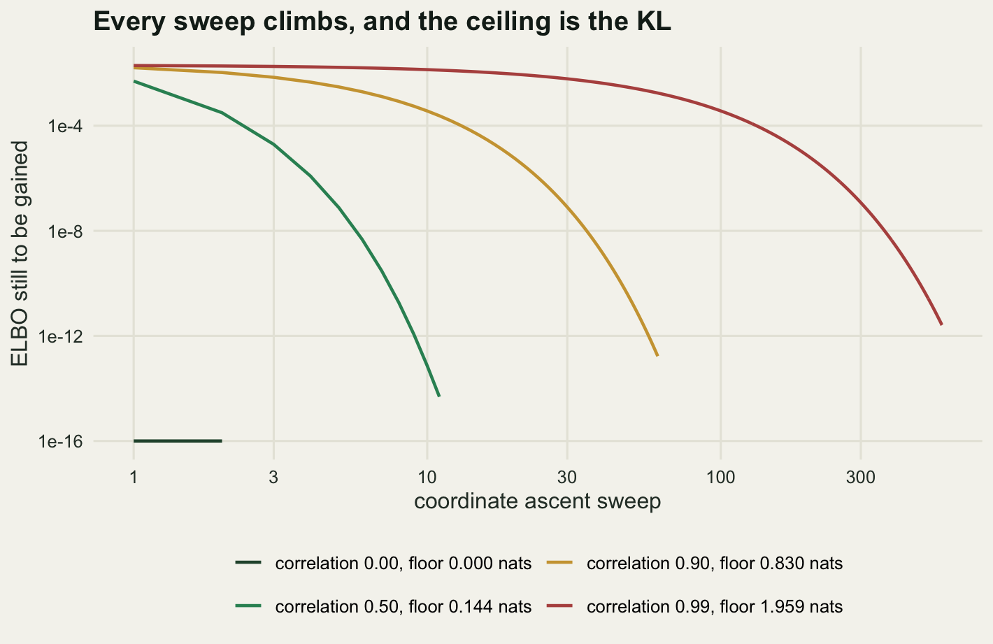
The sweep counts in the table are the second cost of correlation and the one nobody warns you about. Reaching the same tolerance took 2 sweeps at zero correlation and 567 at 0.99. The same off-diagonal term that biases the answer also slows the optimiser down, because each coordinate update chases a target the next update moves.
The correlation the mean field cannot see
Back to the soil depth data, where the correlation is not something I chose.
cen_tab <- data.frame(
  correlation = c(ex_raw$rho, ex_cen$rho),
  exact_sd_slope = c(ex_raw$sd[2], ex_cen$sd[2]),
  vi_sd_slope = c(sqrt(cv_raw$v[2]), sqrt(cv_cen$v[2])),
  exact_sd_intercept = c(ex_raw$sd[1], ex_cen$sd[1]),
  vi_sd_intercept = c(sqrt(cv_raw$v[1]), sqrt(cv_cen$v[1])),
  elbo_gap = c(ex_raw$logz - cv_raw$elbo, ex_cen$logz - cv_cen$elbo),
  predicted_kl = c(-0.5 * log(1 - ex_raw$rho^2), -0.5 * log(1 - ex_cen$rho^2) + 0),
  sweeps = c(cv_raw$sweeps, cv_cen$sweeps),
  row.names = c("depth as measured", "depth centred"))
cen_tab$sd_ratio_slope <- cen_tab$vi_sd_slope / cen_tab$exact_sd_slope
cen_tab$predicted_ratio <- sqrt(1 - cen_tab$correlation^2)

print(round(cen_tab[, c("correlation", "exact_sd_slope", "vi_sd_slope",
                        "sd_ratio_slope", "predicted_ratio")], 6))
correlation exact_sd_slope vi_sd_slope sd_ratio_slope
depth as measured -0.916701 0.017690 0.007069 0.399574
depth centred 0.000000 0.017758 0.017758 1.000000
predicted_ratio
depth as measured 0.399574
depth centred 1.000000print(round(cen_tab[, c("exact_sd_intercept", "vi_sd_intercept", "elbo_gap",
"predicted_kl", "sweeps")], 6)) exact_sd_intercept vi_sd_intercept elbo_gap predicted_kl
depth as measured 0.474505 0.1896 0.917355 0.917355
depth centred 0.189600 0.1896 0.000000 0.000000
sweeps
depth as measured 93
depth centred 2print(round(c(slope_sd_unchanged_by_centring = ex_cen$sd[2] / ex_raw$sd[2],
vi_slope_sd_changed_by_centring = sqrt(cv_cen$v[2]) / sqrt(cv_raw$v[2]),
interval_width_factor = 1 / sqrt(1 - ex_raw$rho^2)), 4)) slope_sd_unchanged_by_centring vi_slope_sd_changed_by_centring
1.0038 2.5122
interval_width_factor
2.5027 With depth as measured, the posterior correlation between the intercept and the slope is -0.9167. The intercept is the biomass predicted at a soil depth of zero, an extrapolation outside the data, so the two coefficients trade off almost perfectly. The variational standard deviation on the slope comes out at 0.007069 against a true 0.01769, a ratio of 0.399574 matching the predicted 0.399574: the honest interval is 2.5027 times as wide as the reported one.
Subtracting the mean depth fixes it. The slope means the same thing in both parametrisations and its exact posterior standard deviation barely moves, multiplied by 1.0038, while the variational standard deviation for that same slope is multiplied by 2.5122. Nothing about the science or the data changed. This is the cheapest fix in the post and it generalises: anything that decorrelates the posterior buys back the variance the mean field discards, whether that is centring a predictor, using sum-to-zero contrasts, or rescaling a covariate whose units make its coefficient tiny.
ell <- function(m, S, p, lab, curve) {
  tt <- seq(0, 2 * pi, length.out = 361)
  z <- cbind(cos(tt), sin(tt)) %*% (chol(S) * sqrt(qchisq(p, 2)))
  data.frame(b0 = m[1] + z[, 1], b1 = m[2] + z[, 2], curve = curve,
             lev = paste0(100 * p, "%"), panel = lab)
}
mk <- function(ex, cv, lab) {
  rbind(ell(ex$mu, ex$Sig, 0.5, lab, "exact posterior"),
        ell(ex$mu, ex$Sig, 0.95, lab, "exact posterior"),
        ell(cv$m, diag(cv$v), 0.5, lab, "mean-field q"),
        ell(cv$m, diag(cv$v), 0.95, lab, "mean-field q"))
}
lab_p <- c("soil depth as measured", "soil depth centred")

cd <- rbind(mk(ex_raw, cv_raw, lab_p[1]), mk(ex_cen, cv_cen, lab_p[2]))
cd$panel <- factor(cd$panel, levels = lab_p)
cd$grp <- paste(cd$curve, cd$lev, cd$panel)
ggplot(cd, aes(b0, b1, colour = curve, linetype = curve, group = grp)) +
  geom_path(linewidth = 0.8) +
  facet_wrap(~panel, scales = "free_x", nrow = 1) +
  scale_colour_manual(values = c(te_pal$forest, te_pal$clay), name = NULL) +
  scale_linetype_manual(values = c("solid", "22"), name = NULL) +
  labs(x = "intercept", y = "slope on soil depth",
       title = "What the mean field cannot represent") +
  theme_te() +
  theme(legend.position = "bottom", plot.margin = margin(8, 16, 4, 8))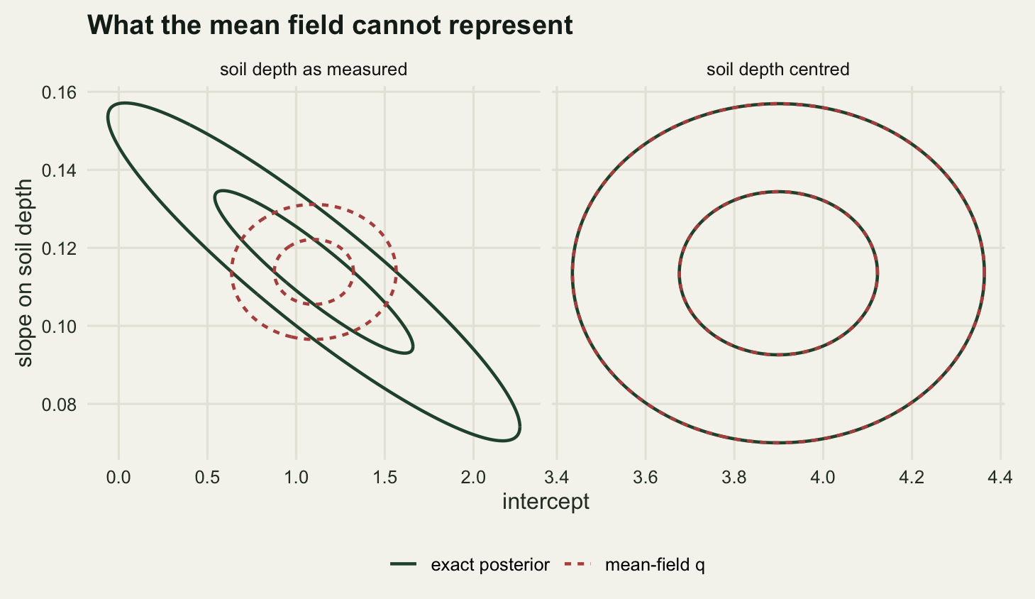
The left panel is the whole problem in one picture. The red ellipse is not a shrunken copy of the green one, and it is not even contained in it: the red contour touches the green one at its four extreme points and pushes outside it towards the upper right and the lower left. The diagonal ridge of the true posterior is exactly the part it cannot follow.
Which way round the divergence goes
Everything above uses the divergence with \(q\) on the left. The other order gives a visibly different answer, and seeing both is the fastest way to understand why variational posteriors behave as they do. The target here is a posterior for an annual log growth rate under a two-regime model, where the data cannot decide which regime dominated: two modes, unequal weights. Minimising \(\text{KL}(q \,\|\, p)\) over Gaussians is what variational inference does; minimising \(\text{KL}(p \,\|\, q)\) has a closed-form answer, the Gaussian matching the first two moments of the target.
mix_w <- c(0.4, 0.6)
mix_m <- c(-1.7, 1.5)
mix_s <- c(0.45, 0.5)

p_dens <- function(x) mix_w[1] * dnorm(x, mix_m[1], mix_s[1]) +
  mix_w[2] * dnorm(x, mix_m[2], mix_s[2])
log_p <- function(x) {
  l1 <- log(mix_w[1]) + dnorm(x, mix_m[1], mix_s[1], log = TRUE)
  l2 <- log(mix_w[2]) + dnorm(x, mix_m[2], mix_s[2], log = TRUE)
  mx <- pmax(l1, l2)
  mx + log(exp(l1 - mx) + exp(l2 - mx))
}
kl_qp <- function(par) {
  mu <- par[1]
  sd <- exp(par[2])
  integrate(function(x) dnorm(x, mu, sd) * (dnorm(x, mu, sd, log = TRUE) - log_p(x)),
            mu - 12 * sd, mu + 12 * sd, rel.tol = 1e-11, subdivisions = 900L)$value
}
nm_twice <- function(start, fn) {
  o <- optim(start, fn, method = "Nelder-Mead", control = list(reltol = 1e-14, maxit = 4000))
  optim(o$par, fn, method = "Nelder-Mead", control = list(reltol = 1e-14, maxit = 4000))
}
fit_rev <- function(start) {
  o <- nm_twice(start, kl_qp)
  c(mu = o$par[1], sd = exp(o$par[2]), kl = o$value)
}
r_left <- fit_rev(c(mix_m[1], log(mix_s[1])))
r_right <- fit_rev(c(mix_m[2], log(mix_s[2])))
r_wide <- fit_rev(c(0, log(2)))
p_m1 <- integrate(function(x) x * p_dens(x), -14, 14, rel.tol = 1e-12)$value
p_m2 <- integrate(function(x) (x - p_m1)^2 * p_dens(x), -14, 14, rel.tol = 1e-12)$value
q_fwd <- c(mu = p_m1, sd = sqrt(p_m2))
q_rev <- r_right[1:2]

pmass_in <- function(q) {
  integrate(p_dens, q[[1]] - qnorm(0.975) * q[[2]], q[[1]] + qnorm(0.975) * q[[2]],
            rel.tol = 1e-11)$value
}
p_peak <- optimize(p_dens, c(-4, 4), maximum = TRUE, tol = 1e-12)$objective
qlow <- function(q) {
  integrate(function(x) dnorm(x, q[[1]], q[[2]]) * (p_dens(x) < 0.05 * p_peak),
            q[[1]] - 14 * q[[2]], q[[1]] + 14 * q[[2]], rel.tol = 1e-9,
            subdivisions = 4000L)$value
}
p_low <- integrate(function(x) p_dens(x) * (p_dens(x) < 0.05 * p_peak), -14, 14,
                   rel.tol = 1e-9, subdivisions = 4000L)$value
right_weight <- integrate(p_dens, 0, 14, rel.tol = 1e-11)$value
print(round(rbind(started_at_left_mode = r_left, started_at_right_mode = r_right,
                  started_wide = r_wide), 6))
mu sd kl
started_at_left_mode -1.697711 0.453765 0.914908
started_at_right_mode 1.498151 0.503165 0.509849
started_wide 1.498151 0.503165 0.509849print(round(c(forward_kl_mu = q_fwd[["mu"]], forward_kl_sd = q_fwd[["sd"]],
exact_posterior_sd = sqrt(p_m2),
sd_ratio_forward_over_reverse = q_fwd[["sd"]] / q_rev[[2]],
reverse_sd_over_exact = q_rev[[2]] / sqrt(p_m2)), 6)) forward_kl_mu forward_kl_sd
0.220000 1.639695
exact_posterior_sd sd_ratio_forward_over_reverse
1.639695 3.258763
reverse_sd_over_exact
0.306865 print(round(c(mass_in_reverse_interval = pmass_in(q_rev),
mass_in_forward_interval = pmass_in(q_fwd),
weight_of_right_mode = right_weight,
reverse_mass_in_empty_region = qlow(q_rev),
forward_mass_in_empty_region = qlow(q_fwd),
posterior_mass_in_empty_region = p_low), 6)) mass_in_reverse_interval mass_in_forward_interval
0.570859 0.999159
weight_of_right_mode reverse_mass_in_empty_region
0.599222 0.014984
forward_mass_in_empty_region posterior_mass_in_empty_region
0.315428 0.016700 Started at the left mode, the reverse divergence fit settles at -1.6977 with a standard deviation of 0.4538 and never leaves. Started at the right mode it settles at 1.4982, and started deliberately wide, spanning both modes, it collapses onto the right mode too and returns 1.4982. Two local optima, and the wide start does not survive: the objective actively pushes mass out of the valley.
The two directions differ by more than a factor of three in scale. The reverse fit has a standard deviation of 0.5032, the forward fit 1.6397, and the true posterior 1.6397, so the reverse fit reports 0.3069 of the real spread.
The mass measurements say what each one bought. The reverse fit’s central 95 per cent interval contains 0.5709 of the posterior, close to the 0.5992 carried by the mode it chose and no more; the forward fit’s contains 0.9992, essentially everything. Then the cost: where the posterior density is under five per cent of its peak, the posterior itself keeps 0.0167 of its mass, the reverse fit 0.015, and the forward fit 0.3154.
Neither is right. The mode-seeking answer is confidently incomplete, the mass-covering answer is diffusely wrong, and variational inference uses the first not because it is better: the forward divergence needs expectations under the posterior, which is the object you did not have.
Where Laplace and the variational fit part company
The mode-seeking behaviour above puts variational inference in the same family as the Laplace approximation, which also fits a Gaussian and also ends up near a mode. A skewed posterior separates them. Take a rare species detected three times in a fixed survey effort with a Gamma prior on the encounter rate, and work on the log rate so the parameter is unconstrained: the posterior is a log gamma, skewed, with a long left tail. Laplace takes the mode and the curvature there; the variational fit minimises the divergence over the same Gaussian family.
y_det <- 3
effort <- 1
prior_shape <- 1
prior_rate <- 0.2
a_post <- prior_shape + y_det
b_post <- prior_rate + effort

log_psk <- function(x) a_post * x - b_post * exp(x) -
  (lgamma(a_post) - a_post * log(b_post))
kl_sk <- function(par) {
  mu <- par[1]
  sd <- exp(par[2])
  integrate(function(x) dnorm(x, mu, sd) * (dnorm(x, mu, sd, log = TRUE) - log_psk(x)),
            mu - 13 * sd, mu + 13 * sd, rel.tol = 1e-12, subdivisions = 1000L)$value
}

o_sk <- nm_twice(c(1, log(0.6)), kl_sk)
o_sk <- nm_twice(o_sk$par, kl_sk)
vi_sk <- c(mu = o_sk$par[1], sd = exp(o_sk$par[2]))
lap_sk <- c(mu = log(a_post / b_post), sd = 1 / sqrt(a_post))
pred_sk <- c(mu = log(a_post / b_post) - 1 / (2 * a_post), sd = 1 / sqrt(a_post))
ex_sk <- c(mean = digamma(a_post) - log(b_post), sd = sqrt(trigamma(a_post)))
kl_lap <- kl_sk(c(lap_sk[[1]], log(lap_sk[[2]])))

print(round(c(detections = y_det, effort = effort, prior_shape = prior_shape,
              prior_rate = prior_rate, posterior_shape = a_post, posterior_rate = b_post,
              exact_mean = ex_sk[["mean"]], exact_sd = ex_sk[["sd"]]), 6))
detections effort prior_shape prior_rate posterior_shape
3.000000 1.000000 1.000000 0.200000 4.000000
posterior_rate exact_mean exact_sd
1.200000 1.073796 0.532750 print(round(c(variational_mu = vi_sk[["mu"]], variational_sd = vi_sk[["sd"]],
analytic_mu = pred_sk[["mu"]], analytic_sd = pred_sk[["sd"]],
laplace_mu = lap_sk[["mu"]], laplace_sd = lap_sk[["sd"]]), 8))variational_mu variational_sd analytic_mu analytic_sd laplace_mu
1.078973 0.500000 1.078973 0.500000 1.203973
laplace_sd
0.500000 print(signif(c(numeric_vs_analytic = max(abs(vi_sk - pred_sk))), 3))numeric_vs_analytic
7.85e-09 print(round(c(location_gap = lap_sk[["mu"]] - vi_sk[["mu"]],
gap_in_exact_sd = (lap_sk[["mu"]] - vi_sk[["mu"]]) / ex_sk[["sd"]],
sd_over_exact_both = lap_sk[["sd"]] / ex_sk[["sd"]],
kl_variational = o_sk$value, kl_laplace = kl_lap,
kl_ratio = kl_lap / o_sk$value,
exact_lower_tail = pgamma(1, a_post, b_post),
laplace_lower_tail = pnorm(0, lap_sk[[1]], lap_sk[[2]]),
variational_lower_tail = pnorm(0, vi_sk[[1]], vi_sk[[2]])), 6)) location_gap gap_in_exact_sd sd_over_exact_both
0.125000 0.234631 0.938526
kl_variational kl_laplace kl_ratio
0.020791 0.053384 2.567713
exact_lower_tail laplace_lower_tail variational_lower_tail
0.033769 0.008021 0.015466 The measurement went somewhere I did not expect. I set out to show that the two mode-seeking Gaussians differ in width, and they do not: both report a standard deviation of exactly 0.5. Differentiating the ELBO explains why. The optimum satisfies \(\sigma_q^2 = 1/a\) and \(\mu_q = \log(a/b) - 1/(2a)\), where \(a\) and \(b\) are the posterior shape and rate, and the Laplace curvature at the mode is also \(a\). The numerical optimisation lands on that prediction to 7.85e-09.
So the two differ only in location, by exactly \(1/(2a)\), here 0.125, or 0.2346 of a posterior standard deviation. The variational fit slides down the shallow side of the skew, away from the mode and towards the mass, and the shift is worth something: its divergence from the posterior is 0.020791 against 0.053384 for Laplace. Both understate the spread by the same 0.9385 of the exact standard deviation, and both understate the left tail badly: against an exact 0.0338 probability that the encounter rate is below one, Laplace says 0.008 and the variational fit 0.0155.
xg <- seq(-4.2, 4.2, length.out = 700)
xs2 <- seq(-0.8, 3.2, length.out = 700)
lv <- c("exact posterior", "reverse KL, min KL(q||p)", "forward KL, min KL(p||q)",
        "Laplace at the mode")
pan <- c("bimodal posterior", "skewed posterior")
kd <- rbind(
  data.frame(x = xg, y = p_dens(xg), curve = lv[1], panel = pan[1]),
  data.frame(x = xg, y = dnorm(xg, q_rev[[1]], q_rev[[2]]), curve = lv[2], panel = pan[1]),
  data.frame(x = xg, y = dnorm(xg, q_fwd[[1]], q_fwd[[2]]), curve = lv[3], panel = pan[1]),
  data.frame(x = xs2, y = exp(log_psk(xs2)), curve = lv[1], panel = pan[2]),
  data.frame(x = xs2, y = dnorm(xs2, vi_sk[[1]], vi_sk[[2]]), curve = lv[2], panel = pan[2]),
  data.frame(x = xs2, y = dnorm(xs2, lap_sk[[1]], lap_sk[[2]]), curve = lv[4], panel = pan[2]))
kd$curve <- factor(kd$curve, levels = lv)
kd$panel <- factor(kd$panel, levels = pan)
ggplot(kd, aes(x, y, colour = curve, linetype = curve)) +
  geom_line(linewidth = 0.85) +
  facet_wrap(~panel, scales = "free", nrow = 1) +
  scale_colour_manual(values = c(te_pal$forest, te_pal$clay, te_pal$gold,
                                 te_pal$green), name = NULL, drop = FALSE) +
  scale_linetype_manual(values = c("solid", "22", "42", "1343"), name = NULL,
                        drop = FALSE) +
  guides(colour = guide_legend(nrow = 2), linetype = guide_legend(nrow = 2)) +
  labs(x = "parameter value", y = "density",
       title = "The divergence has a direction") +
  theme_te() +
  theme(legend.position = "bottom", plot.margin = margin(8, 14, 4, 8))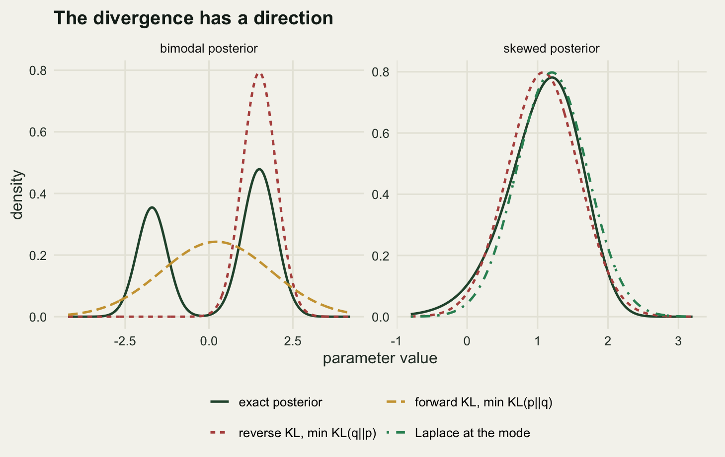
A Poisson mixed model, three ways
Now the model from the opening. Sixteen sites, six visits each, counts with a log link, one observation-level covariate, a random intercept per site, and a lognormal prior on the between-site standard deviation. That prior is not decoration: the profile likelihood for a variance component from sixteen groups sits at zero often enough to matter, as the Laplace post measured, and a prior with no mass at zero keeps the log scale away from minus infinity. The parameter vector is nineteen unknowns and all three fits work on it.
The variational fit uses a mean-field Gaussian over all nineteen. Its ELBO has no intractable piece, because for a Gaussian \(\eta\) the expectation of \(e^{\eta}\) is \(\exp(\mathbb{E}\eta +
\tfrac{1}{2}\text{Var}\,\eta)\), so the Poisson term integrates in closed form and so does everything else. Maximising it is one call to optim. The Laplace fit finds the mode of the same log joint and inverts the Hessian. The reference is a random-walk Metropolis chain with the Laplace covariance as its proposal scale, in the style of Metropolis-Hastings from scratch and Gibbs sampling with conjugate updates.
K_site <- 16
m_vis <- 6
np <- K_site + 3
prior_sd_b <- 2
ls_mu <- log(0.5)
ls_sd <- 1
idx <- c(1, 2, np)
par_names <- c("log_mean_count", "slope", "log_sigma")

sim_glmm <- function(seed, b0 = log(2.2), b1 = 0.45, sg = 0.8) {
  set.seed(seed)
  xs <- as.vector(scale(runif(K_site * m_vis, 0, 1)))
  u <- rnorm(K_site, 0, sg)
  gg <- rep(seq_len(K_site), each = m_vis)
  list(y = rpois(K_site * m_vis, exp(b0 + b1 * xs + u[gg])), g = gg, x = xs,
       truth = c(b0, b1, log(sg)))
}
log_joint <- function(p, d) {
  eta <- p[1] + p[2] * d$x + p[3:(K_site + 2)][d$g]
  sum(d$y * eta - exp(eta) - lgamma(d$y + 1)) +
    sum(dnorm(p[1:2], 0, prior_sd_b, log = TRUE)) +
    sum(dnorm(p[3:(K_site + 2)], 0, exp(p[np]), log = TRUE)) +
    dnorm(p[np], ls_mu, ls_sd, log = TRUE)
}
elbo_glmm <- function(z, d) {
  mm <- z[1:np]
  vv <- exp(z[(np + 1):(2 * np)])
  e_eta <- mm[1] + mm[2] * d$x + mm[2 + d$g]
  v_eta <- vv[1] + vv[2] * d$x^2 + vv[2 + d$g]
  ms <- mm[np]
  vs <- vv[np]
  sum(d$y * e_eta - exp(e_eta + 0.5 * v_eta) - lgamma(d$y + 1)) +
    sum(-0.5 * log(2 * pi * prior_sd_b^2) - (mm[1:2]^2 + vv[1:2]) / (2 * prior_sd_b^2)) +
    sum(-0.5 * log(2 * pi) - ms - 0.5 * exp(-2 * ms + 2 * vs) *
          (mm[3:(K_site + 2)]^2 + vv[3:(K_site + 2)])) +
    (-0.5 * log(2 * pi * ls_sd^2) - 0.5 * ((ms - ls_mu)^2 + vs) / ls_sd^2) +
    0.5 * sum(log(2 * pi * exp(1) * vv))
}
polish <- function(par, f, reltol) {
  for (k in 1:2) par <- optim(par, f, method = "BFGS",
                              control = list(reltol = reltol, maxit = 900))$par
  par
}
fit_vi <- function(d, reltol = 1e-12) {
  cnt <- 0L
  f <- function(z) { cnt <<- cnt + 1L; -elbo_glmm(z, d) }
  z <- polish(c(log(mean(d$y)), 0, rep(0, K_site), ls_mu, rep(log(0.1), np)), f, reltol)
  list(m = z[1:np], sd = exp(0.5 * z[(np + 1):(2 * np)]), evals = cnt)
}
fit_lap <- function(d) {
  cnt <- 0L
  f <- function(p) { cnt <<- cnt + 1L; -log_joint(p, d) }
  p <- polish(c(log(mean(d$y)), 0, rep(0, K_site), ls_mu), f, 1e-13)
  S <- solve(optimHess(p, f))
  list(m = p, sd = sqrt(diag(S)), S = S, evals = cnt)
}
fit_mcmc <- function(d, S_prop, start, n_it, seed, burn) {
  set.seed(seed)
  L <- t(chol(S_prop * 2.4^2 / np))
  cur <- start
  lc <- log_joint(cur, d)
  acc <- 0L
  out <- matrix(NA_real_, n_it, np)
  for (i in seq_len(n_it)) {
    prop <- cur + as.vector(L %*% rnorm(np))
    lp <- log_joint(prop, d)
    if (log(runif(1)) < lp - lc) { cur <- prop; lc <- lp; acc <- acc + 1L }
    out[i, ] <- cur
  }
  list(draws = out[(burn + 1):n_it, , drop = FALSE], acc = acc / n_it, evals = n_it)
}
d1 <- sim_glmm(20260801)
vi1 <- fit_vi(d1)
lp1 <- fit_lap(d1)
mc1 <- fit_mcmc(d1, lp1$S, lp1$m, 160000L, 20260802, 20000L)
dr <- mc1$draws[seq(1, nrow(mc1$draws), by = 10), ]
mc_m <- colMeans(dr)
mc_sd <- apply(dr, 2, sd)
tab <- data.frame(mcmc_mean = mc_m[idx], vi_mean = vi1$m[idx], lap_mean = lp1$m[idx],
mcmc_sd = mc_sd[idx], vi_sd = vi1$sd[idx], lap_sd = lp1$sd[idx],
row.names = par_names)
tab$vi_sd_ratio <- tab$vi_sd / tab$mcmc_sd
tab$lap_sd_ratio <- tab$lap_sd / tab$mcmc_sd
tab$vi_shift <- (tab$vi_mean - tab$mcmc_mean) / tab$mcmc_sd
tab$lap_shift <- (tab$lap_mean - tab$mcmc_mean) / tab$mcmc_sd
pred_ratio <- 1 / (sqrt(diag(solve(cov(dr)))) * mc_sd)
cor_b0_u <- range(cor(dr)[1, 3:(K_site + 2)])
acf_b0 <- acf(dr[, 1], lag.max = 300, plot = FALSE)$acf[-1]
ess_b0 <- nrow(dr) / (1 + 2 * sum(acf_b0[cumsum(acf_b0 < 0) == 0]))
print(round(c(sites = K_site, visits_each = m_vis, counts = length(d1$y),
mean_count = mean(d1$y), max_count = max(d1$y), zero_counts = sum(d1$y == 0),
acceptance = mc1$acc, draws_kept = nrow(dr), ess_log_mean_count = ess_b0), 4)) sites visits_each counts mean_count
16.0000 6.0000 96.0000 2.8646
max_count zero_counts acceptance draws_kept
14.0000 14.0000 0.2609 14000.0000
ess_log_mean_count
1561.6241 print(round(tab[, c("mcmc_mean", "vi_mean", "lap_mean", "vi_shift", "lap_shift")], 5)) mcmc_mean vi_mean lap_mean vi_shift lap_shift
log_mean_count 0.79562 0.80068 0.85062 0.02513 0.27293
slope 0.33089 0.33015 0.32786 -0.01165 -0.04830
log_sigma -0.34050 -0.38598 -0.55671 -0.20406 -0.97023print(round(tab[, c("mcmc_sd", "vi_sd", "lap_sd", "vi_sd_ratio", "lap_sd_ratio")], 5)) mcmc_sd vi_sd lap_sd vi_sd_ratio lap_sd_ratio
log_mean_count 0.20153 0.06030 0.16090 0.29920 0.79839
slope 0.06270 0.05581 0.06249 0.89004 0.99664
log_sigma 0.22284 0.17248 0.21745 0.77401 0.97583print(round(c(predicted_vi_ratio_1 = pred_ratio[idx][1], predicted_vi_ratio_2 = pred_ratio[idx][2],
predicted_vi_ratio_3 = pred_ratio[idx][3],
mean_abs_error_all_19 = mean(abs(pred_ratio - vi1$sd / mc_sd)),
max_abs_error_all_19 = max(abs(pred_ratio - vi1$sd / mc_sd)),
weakest_intercept_effect_correlation = cor_b0_u[2],
strongest_intercept_effect_correlation = cor_b0_u[1]), 4)) predicted_vi_ratio_1 predicted_vi_ratio_2
0.3069 0.8934
predicted_vi_ratio_3 mean_abs_error_all_19
0.8502 0.0241
max_abs_error_all_19 weakest_intercept_effect_correlation
0.0762 -0.3119
strongest_intercept_effect_correlation
-0.7868 print(c(vi_elbo_evaluations = vi1$evals, laplace_log_joint_evaluations = lp1$evals,
metropolis_iterations = mc1$evals)) vi_elbo_evaluations laplace_log_joint_evaluations
2826 2747
metropolis_iterations
160000 Start with the point estimates, because that is where the method earns its reputation. The variational posterior mean for the log mean count is 0.80068 against 0.79562 from the sampler, 0.0251 posterior standard deviations away, and for the slope -0.0116. The Laplace mode is further off in both cases, 0.2729 and -0.0483, and on the log standard deviation it is -0.9702 standard deviations from the posterior mean, which is what happens when you report a mode from a skewed marginal.
The widths are another story. The variational standard deviation on the log mean count is 0.2992 of the sampler’s, on the slope 0.89, and on the log between-site standard deviation 0.774. The damage is concentrated rather than spread: the intercept absorbs almost all of it, the slope almost none.
That concentration is what the Gaussian result from earlier predicts. The intercept correlates with the site random effects it sits under, between -0.7868 and -0.3119, because the data cannot tell a high overall mean from a set of high site effects, while the covariate varies within sites so its slope is nearly free of them. Invert the posterior covariance matrix from the sampler and apply the mean-field rule that the variational variance is the reciprocal of the diagonal of the precision: that predicts 0.3069 for the intercept against the measured 0.2992, and across all 19 parameters predicted and measured differ by 0.0241 on average.
The cost side is what makes the trade tempting: 2826 ELBO evaluations for the variational fit, 2747 log joint evaluations for Laplace, and 160000 Metropolis iterations to deliver an effective sample size of 1562 on the intercept.
One dataset shows the direction of the error. Whether it matters is a question about repeated use, so the next chunk simulates a hundred datasets from the same process and asks how often each method’s 95 per cent interval contains the value that generated the data.
n_rep <- 100L
nominal <- 0.95
zq <- qnorm(0.975)
cov_one <- function(r) {
  d <- sim_glmm(30000 + r)
  v <- fit_vi(d, reltol = 1e-10)
  l <- fit_lap(d)
  mc <- fit_mcmc(d, l$S, l$m, 30000L, 40000 + r, 5000L)
  q <- apply(mc$draws, 2, quantile, probs = c(0.025, 0.975))
  tv <- d$truth
  c(as.numeric(abs(v$m[idx] - tv) < zq * v$sd[idx]),
    as.numeric(abs(l$m[idx] - tv) < zq * l$sd[idx]),
    as.numeric(tv > q[1, idx] & tv < q[2, idx]),
    2 * zq * v$sd[idx], 2 * zq * l$sd[idx], q[2, idx] - q[1, idx])
}
cvm <- t(vapply(seq_len(n_rep), cov_one, numeric(18)))
cvr <- colMeans(cvm)
cov_tab <- matrix(cvr[1:9], 3, 3, byrow = TRUE,
                  dimnames = list(c("variational", "laplace", "metropolis"), par_names))
wid_tab <- matrix(cvr[10:18], 3, 3, byrow = TRUE,
                  dimnames = list(c("variational", "laplace", "metropolis"), par_names))

print(c(replicate_datasets = n_rep, nominal_coverage = nominal))
replicate_datasets nominal_coverage
100.00 0.95 print(round(cov_tab, 4)) log_mean_count slope log_sigma
variational 0.38 0.92 0.84
laplace 0.91 0.94 0.81
metropolis 0.97 0.95 0.91print(round(wid_tab, 4)) log_mean_count slope log_sigma
variational 0.2246 0.2167 0.6740
laplace 0.7175 0.2574 0.9616
metropolis 0.8793 0.2574 0.8684print(round(c(vi_width_over_mcmc_intercept = wid_tab[1, 1] / wid_tab[3, 1],
lap_width_over_mcmc_intercept = wid_tab[2, 1] / wid_tab[3, 1],
vi_width_over_mcmc_slope = wid_tab[1, 2] / wid_tab[3, 2]), 4)) vi_width_over_mcmc_intercept lap_width_over_mcmc_intercept
0.2554 0.8160
vi_width_over_mcmc_slope
0.8418 The sampler covers the generating intercept in 97 per cent of the 100 datasets, the slope in 95 per cent and the log standard deviation in 91 per cent, which is the standard to judge the approximations against rather than the nominal 95. The variational intervals cover the intercept 38 per cent of the time, the Laplace intervals 91 per cent. An interval meant to be wrong one time in twenty is wrong more than three times in five, and the widths say why: 0.2554 of the sampler’s against 0.816 for Laplace.
The slope survives: 92 per cent against the sampler’s 95, with a width ratio of 0.8418. Whether the variational answer is usable is not a property of the model, it is a property of the parameter, and the diagnostic is whether that parameter is correlated with anything else in the posterior.
When it is good enough, measured on the same model
An ecologist rarely reports a coefficient and stops. What leaves the analysis is usually a prediction: the expected count at a site not yet visited, or the probability that such a site falls below a threshold. Those two are affected very differently.
set.seed(20260803)
nd <- nrow(dr)
rep_u <- 40L
sim_lam <- function(b0v, sgv) {
  bb <- rep(b0v, each = rep_u)
  exp(bb + rnorm(length(bb), 0, rep(sgv, each = rep_u)))
}
draw_q <- function(fit) {
  cbind(rnorm(nd, fit$m[1], fit$sd[1]), exp(rnorm(nd, fit$m[np], fit$sd[np])))
}
qv <- draw_q(vi1)
ql <- draw_q(lp1)
lam_mc <- sim_lam(dr[, 1], exp(dr[, np]))
lam_vi <- sim_lam(qv[, 1], qv[, 2])
lam_lp <- sim_lam(ql[, 1], ql[, 2])
thr <- c(2, 1.5, 1, 0.75, 0.5, 0.35, 0.25)
tt <- data.frame(threshold = thr,
                 mcmc = vapply(thr, function(t) mean(lam_mc < t), numeric(1)),
                 vi = vapply(thr, function(t) mean(lam_vi < t), numeric(1)),
                 lap = vapply(thr, function(t) mean(lam_lp < t), numeric(1)))
tt$vi_ratio <- tt$vi / tt$mcmc
tt$lap_ratio <- tt$lap / tt$mcmc

print(round(c(predictive_draws = length(lam_mc),
              mean_expected_count_mcmc = mean(lam_mc),
              mean_expected_count_vi = mean(lam_vi),
              mean_expected_count_laplace = mean(lam_lp),
              vi_percent_error = 100 * (mean(lam_vi) / mean(lam_mc) - 1),
              laplace_percent_error = 100 * (mean(lam_lp) / mean(lam_mc) - 1)), 4))
predictive_draws mean_expected_count_mcmc
560000.0000 3.0147
mean_expected_count_vi mean_expected_count_laplace
2.8557 2.8538
vi_percent_error laplace_percent_error
-5.2738 -5.3373 print(round(tt, 5)) threshold mcmc vi lap vi_ratio lap_ratio
1 2.00 0.44021 0.43750 0.39377 0.99384 0.89450
2 1.50 0.29301 0.27936 0.22544 0.95343 0.76940
3 1.00 0.14211 0.12134 0.08122 0.85390 0.57151
4 0.75 0.07714 0.05909 0.03440 0.76598 0.44600
5 0.50 0.03014 0.01835 0.00911 0.60884 0.30223
6 0.35 0.01238 0.00589 0.00255 0.47627 0.20632
7 0.25 0.00504 0.00185 0.00066 0.36769 0.13107The posterior mean of the expected count at a new site is 3.0147 from the sampler and 2.8557 from the variational fit, an error of -5.274 per cent. For most purposes that is fine, and it is the reason variational methods are used at all. It is also not zero, and the reason is instructive: the expected count is a convex function of the parameters, so the missing posterior variance returns as a downward bias in the mean.
The tail is where it stops being fine. At a threshold of 2 individuals per visit the variational estimate is 0.9938 of the sampler’s; at 1 it is 0.8539, at 0.5 0.6088, and at 0.25 0.3677. The Laplace numbers are worse throughout, from 0.8945 down to 0.1311, because its estimate of the between-site standard deviation is a mode rather than a mean and sits low.
Every entry in both columns is below one. The error is not noise around the right answer, it is a systematic understatement that grows as the threshold moves into the tail, which is the direction a risk calculation travels. If the decision is whether expected abundance is high enough to matter, the variational answer will do. If it is the probability of falling below a management threshold, the risk comes back at under two fifths of what a sampler says, with no sign of trouble anywhere in the fit.
meth <- c("Metropolis", "variational", "Laplace")
dk <- density(dr[, 1], n = 512)
b0g <- seq(min(dk$x), max(dk$x), length.out = 400)
pan_g <- c("posterior for the log mean count", "tail probability, relative to the sampler")
gp <- rbind(
  data.frame(x = dk$x, y = dk$y, method = meth[1], panel = pan_g[1]),
  data.frame(x = b0g, y = dnorm(b0g, vi1$m[1], vi1$sd[1]), method = meth[2], panel = pan_g[1]),
  data.frame(x = b0g, y = dnorm(b0g, lp1$m[1], lp1$sd[1]), method = meth[3], panel = pan_g[1]),
  data.frame(x = tt$threshold, y = rep(1, nrow(tt)), method = meth[1], panel = pan_g[2]),
  data.frame(x = tt$threshold, y = tt$vi_ratio, method = meth[2], panel = pan_g[2]),
  data.frame(x = tt$threshold, y = tt$lap_ratio, method = meth[3], panel = pan_g[2]))
gp$method <- factor(gp$method, levels = meth)
gp$panel <- factor(gp$panel, levels = pan_g)
ggplot(gp, aes(x, y, colour = method, linetype = method)) +
  geom_line(linewidth = 0.85) +
  facet_wrap(~panel, scales = "free", nrow = 1) +
  scale_colour_manual(values = c(te_pal$forest, te_pal$clay, te_pal$gold), name = NULL) +
  scale_linetype_manual(values = c("solid", "22", "42"), name = NULL) +
  labs(x = "log mean count (left panel) and threshold on expected count (right panel)",
       y = NULL, title = "Good centre, wrong width, worse tail") +
  theme_te() +
  theme(legend.position = "bottom", plot.margin = margin(8, 14, 4, 8))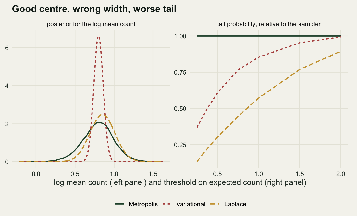
What to take away
The method is one identity and one loop: the ELBO plus the divergence equals the log marginal likelihood, and coordinate ascent raises the first by lowering the second. On a conjugate posterior that factorises the loop returned the exact answer, an ELBO gap of 0 and a standard deviation error of 0. Where it does not factorise, the shortfall matched the analytic divergence to 2.59e-12 and the shrinkage matched \(\sqrt{1-\rho^2}\) to 9.16e-16 across the whole sweep.
That formula is the practical content. The variance you lose is a function of the correlation you ignore, so you can predict the damage before fitting anything, and often remove it. Centring the soil depth predictor took the intercept and slope correlation from -0.9167 to 0, multiplied the reported standard deviation on the slope by 2.5122 while the true value moved by a factor of 1.0038, and cut the sweeps to convergence from 93 to 2.
Two measurements went against what I set out to show. On the skewed posterior I expected the variational and the Laplace fit to disagree about width; they agree exactly, both returning 0.5, and the whole difference is a location shift of 0.125 that the algebra gives as \(1/(2a)\). In the mixed model I expected the variance loss to be spread over the parameters; it was not. The intercept kept 0.2992 of its uncertainty and the slope 0.89, and the coverage followed: 38 per cent against 92 per cent.
The honest limit is not the bias itself, since a measured bias with a formula attached is manageable. It is that nothing inside the fit reports it. The ELBO is a lower bound on a quantity you do not know, so its value says nothing about how tight it is: at a correlation of 0.99 the converged ELBO was 1.9585 nats short of the truth and looked exactly as converged as the run at zero correlation, which was short by 0. Every diagnosis here came from outside the method. In practice that means running a sampler once, on one representative dataset, to measure the ratio between the variational interval and the honest one, then using the variational fit everywhere with that ratio in hand. Used without it, the fit is fast, well behaved, plausible, and too confident by a factor you never see.
References
Blei DM, Kucukelbir A, McAuliffe JD 2017 Journal of the American Statistical Association 112(518):859-877 (10.1080/01621459.2017.1285773)
Jordan MI, Ghahramani Z, Jaakkola TS, Saul LK 1999 Machine Learning 37(2):183-233 (10.1023/A:1007665907178)
Ormerod JT, Wand MP 2010 The American Statistician 64(2):140-153 (10.1198/tast.2010.09058)
Turner RE, Sahani M 2011 Bayesian Time Series Models, Cambridge University Press:104-124 (10.1017/CBO9780511984679.006)
Wang Y, Blei DM 2019 Journal of the American Statistical Association 114(527):1147-1161 (10.1080/01621459.2018.1473776)
Rue H, Martino S, Chopin N 2009 Journal of the Royal Statistical Society Series B 71(2):319-392 (10.1111/j.1467-9868.2008.00700.x)
Hui FKC, Warton DI, Ormerod JT, Haapaniemi V, Taskinen S 2017 Journal of Computational and Graphical Statistics 26(1):35-43 (10.1080/10618600.2016.1164708)
Niku J, Hui FKC, Taskinen S, Warton DI 2019 Methods in Ecology and Evolution 10(12):2173-2182 (10.1111/2041-210X.13303)
Bolker BM, Brooks ME, Clark CJ, Geange SW, Poulsen JR, Stevens MHH, White JSS 2009 Trends in Ecology and Evolution 24(3):127-135 (10.1016/j.tree.2008.10.008)