library(ggplot2)

te_pal <- list(forest = "#275139", green = "#2f8f63", sage = "#93a87f",
               clay = "#b5534e", gold = "#cda23f", line = "#dad9ca",
               ink = "#16241d", paper = "#f5f4ee")

theme_te <- function() {
  theme_minimal(base_size = 12) +
    theme(panel.grid.minor = element_blank(),
          panel.grid.major = element_line(colour = "#e7e6dc"),
          plot.background = element_rect(fill = "#f5f4ee", colour = NA),
          panel.background = element_rect(fill = "#f5f4ee", colour = NA),
          plot.title = element_text(face = "bold", colour = te_pal$ink),
          axis.title = element_text(colour = "#2c3a31"),
          legend.position = "bottom")
}The Laplace approximation in R
R
MCMC
Bayesian statistics
model selection
ecology tutorial
Fit a Gaussian at the posterior mode in base R: marginal likelihoods, where the approximation is excellent, and the three ways it fails in ecological models.
The reason a mixed model fits in a second while an MCMC run takes minutes is a two-hundred-year-old trick with a Gaussian in it. Somewhere inside lme4, inside glmmTMB, inside mgcv when the smoothing parameters are chosen by marginal likelihood, and inside every INLA fit, there is a loop that finds the maximum of a log density and then measures the curvature there. Everything downstream is arithmetic on those two objects.
Knowing what that loop does matters, because the packages that use it are the ones ecologists reach for first, and because its failure modes are not random. They are three specific shapes of posterior, all of which turn up in real analyses: a skewed posterior from a small binomial sample, a variance component whose mass piles against zero, and a likelihood with two modes. Each fails in its own way, and only one of the three announces itself.
Consider a set of pitfall traps along an elevational gradient, counts of a ground beetle at sixty sites, and the question of whether abundance changes with elevation. There is a posterior over two coefficients somewhere in that problem. A sampler would draw from it. A Laplace approximation instead finds the single highest point, measures how sharply the log density falls away, and declares the answer to be the Gaussian with that peak and that curvature. Three lines of base R once you have a mode and a Hessian.
This post writes all of it out. It builds the approximation, derives its marginal likelihood, and checks that against two models with an exact closed-form answer so the error is measured rather than asserted. Then it sweeps sample size to find the rate at which each part of the answer converges, and finds that the parts do not converge in the order most people would guess. Then it breaks the approximation three ways on purpose and measures the damage.
Two earlier posts are the natural neighbours: Metropolis-Hastings from scratch and Hamiltonian Monte Carlo from scratch reach the same posterior by sampling rather than by curvature, and are the reference the approximation gets checked against when there is no exact answer. Bayesian model comparison: WAIC, LOO, DIC compares models without a marginal likelihood at all.
A Gaussian at the mode
Write the unnormalised log posterior as \(\ell(\theta) = \log p(y \mid \theta) + \log p(\theta)\) and expand it in a Taylor series about its maximum \(\hat\theta\). The linear term vanishes because the gradient is zero at a maximum, so to second order
\[\ell(\theta) \approx \ell(\hat\theta) - \tfrac{1}{2}(\theta - \hat\theta)^{\top} H (\theta - \hat\theta), \qquad H = -\nabla^2 \ell(\hat\theta)\]
and exponentiating gives a Gaussian kernel with mean \(\hat\theta\) and covariance \(H^{-1}\). That is the whole approximation. \(H\) is the Hessian of the negative log posterior at the mode, and it is the only thing besides the mode itself that the method ever looks at.
The beetle counts give a two-parameter example: sixty sites, a standardised elevation covariate, Poisson counts with a log link, and an independent normal prior on each coefficient. optim finds the mode and optimHess returns a numerical Hessian, but for this model the Hessian is also available in closed form. It is \(X^{\top} W X\) plus the prior precision, where \(W\) is diagonal with the fitted means on it. Computing it both ways is the cheapest sanity check there is.
set.seed(20260728)
n_site <- 60
elev <- as.vector(scale(runif(n_site, 0, 1)))
X <- cbind(1, elev)
tau2 <- 4
b_true <- c(1.4, 0.8)
y_cnt <- rpois(n_site, exp(b_true[1] + b_true[2] * elev))

neg_log_post <- function(bv) {
  eta <- as.vector(X %*% bv)
  -sum(y_cnt * eta - exp(eta) - lgamma(y_cnt + 1)) +
    0.5 * sum(bv^2) / tau2 + log(2 * pi * tau2)
}

fit_pois <- optim(c(0, 0), neg_log_post, method = "BFGS")
mode_hat <- fit_pois$par
H_num <- optimHess(mode_hat, neg_log_post)

wts <- exp(as.vector(X %*% mode_hat))
H_ana <- t(X) %*% (X * wts) + diag(2) / tau2
post_sd <- unname(sqrt(diag(solve(H_ana))))
hess_abs <- max(abs(H_num - H_ana))
hess_rel <- max(abs(H_num - H_ana) / abs(H_ana))

print(round(c(n_sites = n_site, prior_variance = tau2,
              true_intercept = b_true[1], true_slope = b_true[2],
              mode_intercept = mode_hat[1], mode_slope = mode_hat[2],
              sd_intercept = post_sd[1], sd_slope = post_sd[2],
              optim_fn_evals = fit_pois$counts[["function"]]), 4))
n_sites prior_variance true_intercept true_slope mode_intercept
60.0000 4.0000 1.4000 0.8000 1.5070
mode_slope sd_intercept sd_slope optim_fn_evals
0.7293 0.0677 0.0643 40.0000 print(round(H_ana, 4)) elev
346.8732 222.0327
elev 222.0327 384.0035print(round(c(hessian_max_abs_diff = hess_abs), 6))hessian_max_abs_diff
2e-04 print(signif(c(hessian_max_rel_diff = hess_rel), 3))hessian_max_rel_diff
5.22e-07 The mode sits at 1.507 for the intercept and 0.7293 for the elevation slope, with approximate posterior standard deviations 0.0677 and 0.0643. The generating values were 1.4 and 0.8, so the approximation recovered them to within about one and a half posterior standard deviations (1.6 and 1.1), which is what sixty Poisson counts are worth.
The two Hessians agree to 2e-04 in absolute terms and to 5.22e-07 in relative terms. That gap is not error in the approximation; it is the finite-difference step optimHess uses, and it says the numerical route is fine for a model where you cannot face writing the derivatives out. The whole approximate posterior is now two objects, mode_hat and H_ana.
Note what the log link bought. The coefficients live on the whole real line and the prior keeps them from running away, so the posterior has an interior maximum with finite curvature there. Every failure below is a case where one of those two conditions does not hold.
The marginal likelihood, and two exact checks
The same expansion gives the normalising constant. Integrate the second-order approximation over \(\theta\): the integral of a Gaussian kernel in \(d\) dimensions is \((2\pi)^{d/2} |H|^{-1/2}\), so
\[\log p(y) \approx \ell(\hat\theta) + \frac{d}{2}\log(2\pi) - \frac{1}{2}\log |H|\]
with \(|H|\) the determinant. That is the Laplace approximation to the marginal likelihood, and it is the reason marginal likelihoods are computable at all in most real problems. An exact marginal likelihood is a \(d\)-dimensional integral over the whole parameter space; this formula replaces it with one optimisation and one determinant.
There is one family where the approximation is not an approximation. If the posterior is exactly Gaussian, the second-order expansion is the function itself and the formula is exact. A linear model with known residual variance and a Gaussian prior on the coefficients is such a case, and it also has a closed-form marginal likelihood, because marginally \(y \sim N(0,\, X \Sigma_0 X^{\top} + \sigma^2 I)\).
set.seed(20260729)
n_seq <- c(5, 10, 20, 40, 80, 160, 320, 640, 1280, 2560)

gauss_check <- function(n_obs) {
  xg <- as.vector(scale(runif(n_obs, 0, 1)))
  Xg <- cbind(1, xg)
  s2 <- 0.8
  S0 <- diag(c(4, 4))
  yg <- as.vector(Xg %*% c(1.2, -0.7)) + rnorm(n_obs, 0, sqrt(s2))
  nlp <- function(bv) {
    r <- yg - as.vector(Xg %*% bv)
    0.5 * sum(r^2) / s2 + 0.5 * as.numeric(bv %*% solve(S0, bv)) +
      0.5 * n_obs * log(2 * pi * s2) + 0.5 * log(det(2 * pi * S0))
  }
  o <- optim(c(0, 0), nlp, method = "BFGS", control = list(reltol = 1e-14))
  Hg <- t(Xg) %*% Xg / s2 + solve(S0)
  lap <- -nlp(o$par) + log(2 * pi) - 0.5 * log(det(Hg))
  Vm <- Xg %*% S0 %*% t(Xg) + s2 * diag(n_obs)
  ex <- -0.5 * (n_obs * log(2 * pi) + as.numeric(determinant(Vm)$modulus) +
                  as.numeric(yg %*% solve(Vm, yg)))
  c(laplace = lap, exact = ex, error = lap - ex)
}

gauss_tab <- as.data.frame(t(vapply(n_seq, gauss_check, numeric(3))))
gauss_tab$n <- n_seq
gauss_worst <- max(abs(gauss_tab$error))
print(round(gauss_tab[c(1, 5, 10), c("n", "laplace", "exact")], 4))
n laplace exact
1 5 -9.1195 -9.1195
5 80 -115.6360 -115.6360
10 2560 -3324.5993 -3324.5993print(signif(c(worst_absolute_error = gauss_worst), 3))worst_absolute_error
3.18e-12 print(c(models_checked = length(n_seq)))models_checked
10 Across 10 sample sizes from 5 to 2560, the worst disagreement between the Laplace marginal likelihood and the exact one is 3.18e-12. That is eleven decimal places of agreement, and what is left is rounding in double precision, not the approximation. When the posterior is Gaussian, the Laplace formula returns the truth.
That is a useful calibration point: it says the error is entirely a statement about non-Gaussianity, and its size measures how far from Gaussian the posterior strayed.
The second check has a real error in it. The beta-binomial has an exact marginal likelihood that Laplace does not reproduce. With \(y\) successes in \(n\) trials and a \(\text{Beta}(a,b)\) prior, the marginal likelihood is a ratio of beta functions. Working on the log-odds scale to keep the parameter unconstrained, the log joint is \((y+a)\theta - (n+a+b)\log(1 + e^{\theta})\) plus a constant, whose mode and curvature are both available in closed form: the mode sits at \(p^{*} = (y+a)/(n+a+b)\) and the curvature is \((n+a+b)\,p^{*}(1-p^{*})\).
lap_marg_bb <- function(y, n, a = 1, b = 1) {
  A <- y + a
  B <- n - y + b
  th <- log(A / B)
  p_star <- A / (A + B)
  lj <- lchoose(n, y) - lbeta(a, b) + A * th - (A + B) * log1p(exp(th))
  lj + 0.5 * log(2 * pi) - 0.5 * log((A + B) * p_star * (1 - p_star))
}

ex_marg_bb <- function(y, n, a = 1, b = 1) {
  lchoose(n, y) + lbeta(a + y, b + n - y) - lbeta(a, b)
}

p_true <- 0.25
bb <- data.frame(n = n_seq, y = round(p_true * n_seq))
bb$exact <- ex_marg_bb(bb$y, bb$n)
bb$laplace <- lap_marg_bb(bb$y, bb$n)
bb$error <- bb$laplace - bb$exact
print(round(bb, 6))
n y exact laplace error
1 5 1 -1.791759 -1.837848 -0.046089
2 10 2 -2.397895 -2.427886 -0.029991
3 20 5 -3.044522 -3.059819 -0.015296
4 40 10 -3.713572 -3.721850 -0.008278
5 80 20 -4.394449 -4.398767 -0.004318
6 160 40 -5.081404 -5.083611 -0.002207
7 320 80 -5.771441 -5.772557 -0.001116
8 640 160 -6.463029 -6.463591 -0.000561
9 1280 320 -7.155396 -7.155678 -0.000281
10 2560 640 -7.848153 -7.848294 -0.000141keep_m <- bb$n >= 40
slope_marg <- unname(coef(lm(log(abs(error)) ~ log(n), data = bb[keep_m, ]))[2])
mk_series <- function(pp, lab) {
yy <- round(pp * n_seq)
data.frame(n = n_seq, model = lab,
err = abs(lap_marg_bb(yy, n_seq) - ex_marg_bb(yy, n_seq)))
}
marg_dat <- rbind(mk_series(0.25, "binomial, 25% positive"),
mk_series(0.05, "binomial, 5% positive"),
data.frame(n = n_seq, model = "conjugate Gaussian",
err = pmax(abs(gauss_tab$error), 1e-16)))
err25 <- marg_dat$err[marg_dat$model == "binomial, 25% positive"]
err05 <- marg_dat$err[marg_dat$model == "binomial, 5% positive"]
print(round(c(fitted_slope = slope_marg), 3))fitted_slope
-0.982 print(round(c(error_at_smallest_n = bb$error[1],
error_at_largest_n = bb$error[10],
rare_over_common_error = err05[10] / err25[10]), 5)) error_at_smallest_n error_at_largest_n rare_over_common_error
-0.04609 -0.00014 4.59835 At five trials with one success the Laplace log marginal likelihood is -0.04609 below the exact value, and at 2560 trials with 640 successes it is -0.00014 below. Fitting a line through the logarithms of the absolute errors from 40 trials upward gives a slope of -0.982, the textbook \(O(1/n)\) rate.
The sign matters. Every error in the column is negative: the approximation understates the marginal likelihood at every sample size tested, so the error is a bias rather than noise, and in a model comparison the biases of two competing models need not cancel.
The figure below puts three model families on one pair of log axes: the beta-binomial with a quarter of trials positive, the same model with a twentieth positive, and the conjugate Gaussian from the previous section. The rare counts are rounded to whole trials, so the second series has no positives at all at the two smallest sample sizes.
ggplot(marg_dat, aes(n, err, colour = model, shape = model)) +
  geom_line(linewidth = 0.6) +
  geom_point(size = 2) +
  scale_x_log10(breaks = c(5, 20, 80, 320, 1280)) +
  scale_y_log10(breaks = 10^c(-16, -13, -10, -7, -4, -1),
                labels = c("1e-16", "1e-13", "1e-10", "1e-7", "1e-4", "0.1")) +
  scale_colour_manual(values = c(te_pal$forest, te_pal$clay, te_pal$gold),
                      name = NULL) +
  scale_shape_manual(values = c(16, 17, 15), name = NULL) +
  labs(x = "sample size n", y = "absolute error in log marginal likelihood",
       title = "Laplace marginal likelihood against the exact value") +
  theme_te()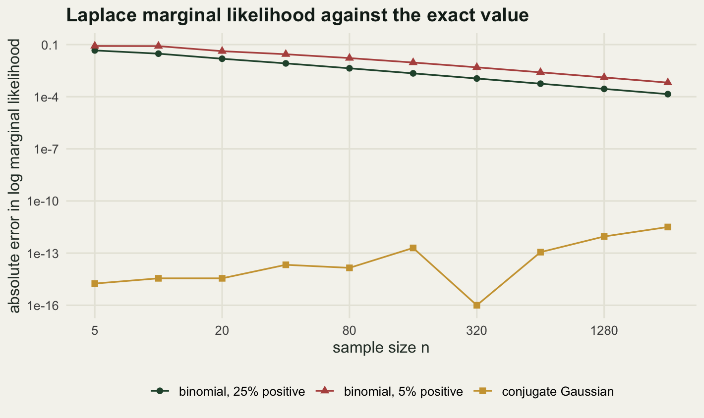
The two binomial lines descend at close to the same rate, so the order of convergence does not depend on how extreme the proportion is, but the rarer species sits above the commoner one at every sample size, and the gap between them widens from left to right instead of holding fixed. At the largest sample size the five per cent model has 4.59835 times the error of the twenty-five per cent model, against 2.72744 times at the smallest size where the rare series has any positives, so the multiplier is itself still settling. The constant in front of the rate depends on how skewed the posterior is, and at the right-hand end of the panel it is also roughly how many extra trials the rare model needs for the same accuracy.
The gold series drifts upward at the largest sample sizes. That is rounding, not the approximation: the log marginal likelihood itself grows with the sample size, and the exact route reaches it through an n by n covariance matrix. The two routes agree only to the last digit a double can carry, so the gap in absolute terms grows along with the number. At this accuracy the reported error is a property of the floating point representation rather than of the mathematics.
What converges first
The marginal likelihood is one number. The posterior summaries are what readers of a paper actually see, and they do not all converge at the same speed. On the log-odds scale the exact posterior mean is \(\psi(A) - \psi(B)\) and the exact variance is \(\psi'(A) + \psi'(B)\), where \(A =
y + a\) and \(B = n - y + b\), and the exact quantiles come from qbeta through qlogis. The Laplace answers are the mode \(\log(A/B)\), the standard deviation \(\sqrt{1/A + 1/B}\), and the mode plus the upper normal quantile times that standard deviation.
The counts below are set to their expected value at each sample size rather than drawn at random, so what the sweep measures is approximation error and not sampling noise.
A_v <- bb$y + 1
B_v <- bb$n - bb$y + 1
rt <- data.frame(n = bb$n,
                 mean_exact = digamma(A_v) - digamma(B_v),
                 mean_lap = log(A_v / B_v),
                 sd_exact = sqrt(trigamma(A_v) + trigamma(B_v)),
                 sd_lap = sqrt(1 / A_v + 1 / B_v))
rt$q_exact <- qlogis(qbeta(0.975, A_v, B_v))
rt$q_lap <- rt$mean_lap + qnorm(0.975) * rt$sd_lap
rt$err_mean <- abs(rt$mean_lap - rt$mean_exact)
rt$err_sd <- abs(rt$sd_lap - rt$sd_exact)
rt$err_q975 <- abs(rt$q_lap - rt$q_exact)
print(round(rt[, c("n", "mean_exact", "mean_lap", "sd_exact", "sd_lap",
                   "q_exact", "q_lap")], 4))
n mean_exact mean_lap sd_exact sd_lap q_exact q_lap
1 5 -1.0833 -0.9163 0.9307 0.8367 0.5807 0.7235
2 10 -1.2179 -1.0986 0.7159 0.6667 0.0711 0.2080
3 20 -1.0349 -0.9808 0.4958 0.4787 -0.1135 -0.0426
4 40 -1.0660 -1.0361 0.3577 0.3510 -0.3928 -0.3482
5 80 -1.0821 -1.0664 0.2555 0.2530 -0.5960 -0.5705
6 160 -1.0903 -1.0822 0.1816 0.1807 -0.7419 -0.7280
7 320 -1.0945 -1.0903 0.1288 0.1284 -0.8459 -0.8386
8 640 -1.0965 -1.0945 0.0912 0.0911 -0.9198 -0.9160
9 1280 -1.0976 -1.0965 0.0645 0.0645 -0.9721 -0.9702
10 2560 -1.0981 -1.0976 0.0456 0.0456 -1.0092 -1.0082print(round(rt[, c("n", "err_mean", "err_sd", "err_q975")], 6)) n err_mean err_sd err_q975
1 5 0.167043 0.094069 0.142806
2 10 0.119245 0.049187 0.136977
3 20 0.054066 0.017086 0.070914
4 40 0.029927 0.006750 0.044549
5 80 0.015779 0.002531 0.025529
6 160 0.008107 0.000922 0.013877
7 320 0.004109 0.000331 0.007313
8 640 0.002069 0.000118 0.003782
9 1280 0.001038 0.000042 0.001934
10 2560 0.000520 0.000015 0.000981keep_r <- rt$n >= 40
slope_of <- function(e) unname(coef(lm(log(e[keep_r]) ~ log(rt$n[keep_r])))[2])
slopes <- c(mean = slope_of(rt$err_mean), sd = slope_of(rt$err_sd),
q975 = slope_of(rt$err_q975))
thr <- 0.01
first_under <- function(e) rt$n[which(e < thr)[1]]
print(round(slopes, 3)) mean sd q975
-0.977 -1.475 -0.923 print(round(c(threshold = thr, first_n_mean_under = first_under(rt$err_mean),
first_n_sd_under = first_under(rt$err_sd),
first_n_tail_under = first_under(rt$err_q975)), 3)) threshold first_n_mean_under first_n_sd_under first_n_tail_under
0.01 160.00 40.00 320.00 print(round(c(tail_over_mean_at_largest_n = rt$err_q975[10] / rt$err_mean[10],
tail_over_sd_at_n40 = rt$err_q975[4] / rt$err_sd[4]), 3))tail_over_mean_at_largest_n tail_over_sd_at_n40
1.887 6.600 print(round(c(tail_err_in_sd_units = rt$err_q975[10] / rt$sd_exact[10],
sd_err_in_sd_units = rt$err_sd[10] / rt$sd_exact[10]), 5))tail_err_in_sd_units sd_err_in_sd_units
0.02150 0.00032 lab_r <- c(sprintf("posterior mean (slope %.2f)", slopes[["mean"]]),
sprintf("posterior SD (slope %.2f)", slopes[["sd"]]),
sprintf("97.5%% quantile (slope %.2f)", slopes[["q975"]]))
rate_long <- data.frame(
n = rep(rt$n, 3),
err = c(rt$err_mean, rt$err_sd, rt$err_q975),
quantity = factor(rep(lab_r, each = nrow(rt)), levels = lab_r))
ggplot(rate_long, aes(n, err, colour = quantity, shape = quantity)) +
geom_line(linewidth = 0.6) +
geom_point(size = 2.1) +
scale_x_log10(breaks = c(5, 20, 80, 320, 1280)) +
scale_y_log10(breaks = 10^(-5:0),
labels = parse(text = paste0("10^", -5:0))) +
scale_colour_manual(values = c(te_pal$forest, te_pal$gold, te_pal$clay),
name = NULL) +
scale_shape_manual(values = c(16, 15, 17), name = NULL) +
guides(colour = guide_legend(nrow = 2), shape = guide_legend(nrow = 2)) +
labs(x = "sample size n", y = "absolute error on the log-odds scale",
title = "What converges first") +
theme_te()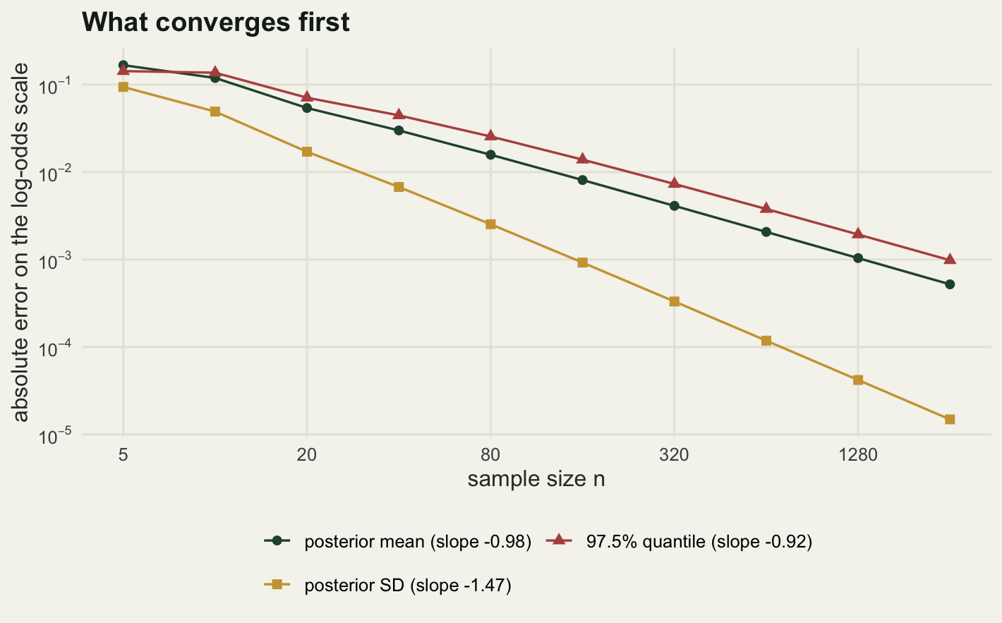
The fitted exponents are -0.977 for the posterior mean, -1.475 for the posterior standard deviation and -0.923 for the upper quantile. The standard deviation is the clear winner: its error falls faster than \(1/n\), close to \(n^{-3/2}\), and by 40 trials it is already under 0.01 on the log-odds scale.
Here the measurement disagrees with the story I set out to tell. The obvious expectation is that both central summaries converge faster than the tail, and that is not what the numbers say. The posterior mean and the tail quantile fall at essentially the same rate, -0.977 against -0.923, both within rounding distance of \(1/n\). What separates them is the constant, not the exponent: at the largest sample size the tail error is 1.887 times the error in the mean, and that ratio climbs down the table rather than shrinking. The tail is not asymptotically worse, it is worse at every sample size past the smallest, by a factor that settles near two.
The practical consequence survives the correction. The posterior mean needs 160 trials to get its error under 0.01, the standard deviation needs only 40, and the upper quantile needs 320. At 40 trials the tail error is already 6.6 times the standard deviation error, so a summary table can look settled while the interval endpoint, the number a threshold decision uses, is nowhere near it. At the largest sample size the tail error is 0.0215 of a posterior standard deviation while the standard deviation error is 0.00032 of one.
If the quantity that matters is a mean, the approximation reaches useful accuracy early. If it is the upper bound on a decline rate, it reaches it later, and the summary table gives no hint of which regime you are in.
Failure one: skew, and a scale that partly repairs it
Now the small samples, where ecology actually lives. A rare plant is searched for at ten quadrats and found in one. With a uniform prior the posterior on occupancy is \(\text{Beta}(2, 10)\), and its exact 95 per cent interval comes straight from qbeta.
The approximation has to be built on some scale, and the choice is not neutral: a Gaussian on the probability scale is a different object from a Gaussian on the log-odds scale pushed back through the inverse logit. Four scales are compared below, each with its log density written out analytically, its mode found by optimise and its curvature by a central difference.
y_s <- 1
n_s <- 10
A_s <- y_s + 1
B_s <- n_s - y_s + 1
ex_int <- qbeta(c(0.025, 0.975), A_s, B_s)

ld_prob  <- function(s) (A_s - 1) * log(s) + (B_s - 1) * log1p(-s)
ld_logit <- function(s) A_s * s - (A_s + B_s) * log1p(exp(s))
ld_asin  <- function(s) (2 * A_s - 1) * log(sin(s)) + (2 * B_s - 1) * log(cos(s))
ld_cube  <- function(s) (3 * A_s - 1) * log(s) + (B_s - 1) * log1p(-s^3)

lap_on <- function(ld, lo, hi, back) {
  o <- optimise(ld, c(lo, hi), maximum = TRUE, tol = 1e-12)
  s0 <- o$maximum
  hstep <- 1e-4
  Hs <- -(ld(s0 + hstep) - 2 * ld(s0) + ld(s0 - hstep)) / hstep^2
  ends <- sort(back(s0 + qnorm(c(0.025, 0.975)) / sqrt(Hs)))
  c(mode_p = back(s0), lo = ends[1], hi = ends[2])
}

skew_of <- function(tf) {
  fd <- function(p) dbeta(p, A_s, B_s)
  m1 <- integrate(function(p) tf(p) * fd(p), 0, 1, rel.tol = 1e-10)$value
  m2 <- integrate(function(p) (tf(p) - m1)^2 * fd(p), 0, 1, rel.tol = 1e-10)$value
  m3 <- integrate(function(p) (tf(p) - m1)^3 * fd(p), 0, 1, rel.tol = 1e-10)$value
  m3 / m2^1.5
}

sk <- data.frame(scale = c("probability", "log-odds", "arcsine root", "cube root"),
                 rbind(lap_on(ld_prob, 1e-8, 1 - 1e-8, function(s) s),
                       lap_on(ld_logit, -20, 20, plogis),
                       lap_on(ld_asin, 1e-8, pi / 2 - 1e-8, function(s) sin(s)^2),
                       lap_on(ld_cube, 1e-8, 1 - 1e-8, function(s) s^3)),
                 row.names = NULL)
sk$skew <- c(skew_of(function(p) p), skew_of(qlogis),
             skew_of(function(p) asin(sqrt(p))), skew_of(function(p) p^(1 / 3)))
sk$centre_shift <- (sk$lo + sk$hi) / 2 - mean(ex_int)
sk$width_ratio <- (sk$hi - sk$lo) / diff(ex_int)
sk$max_abs_err <- pmax(abs(sk$lo - ex_int[1]), abs(sk$hi - ex_int[2]))

print(round(c(trials = n_s, detections = y_s, beta_a = A_s, beta_b = B_s,
              interval_percent = 95,
              exact_lo = ex_int[1], exact_hi = ex_int[2],
              exact_width = diff(ex_int),
              exact_median = qbeta(0.5, A_s, B_s)), 4))
trials detections beta_a beta_b
10.0000 1.0000 2.0000 10.0000
interval_percent exact_lo exact_hi exact_width
95.0000 0.0228 0.4128 0.3899
exact_median
0.1480 print(round(sk[, c("mode_p", "lo", "hi", "skew", "centre_shift",
"width_ratio", "max_abs_err")], 4)) mode_p lo hi skew centre_shift width_ratio max_abs_err
1 0.1000 -0.0859 0.2859 0.9214 -0.1178 0.9537 0.1268
2 0.1667 0.0420 0.4772 -0.6050 0.0418 1.1161 0.0644
3 0.1364 0.0068 0.3892 0.3076 -0.0198 0.9806 0.0235
4 0.1562 0.0239 0.4911 -0.1672 0.0397 1.1981 0.0783print(sk$scale)[1] "probability" "log-odds" "arcsine root" "cube root" print(round(c(pct_removed_vs_probability =
100 * (1 - sk$max_abs_err[3] / sk$max_abs_err[1]),
pct_removed_vs_logodds =
100 * (1 - sk$max_abs_err[3] / sk$max_abs_err[2])), 1))pct_removed_vs_probability pct_removed_vs_logodds
81.4 63.4 print(round(c(shift_as_fraction_of_width =
abs(sk$centre_shift[1]) / diff(ex_int)), 4))shift_as_fraction_of_width
0.3021 The exact interval runs from 0.0228 to 0.4128, a width of 0.3899. On the probability scale the approximation returns -0.0859 to 0.2859. The lower endpoint is a negative occupancy probability, which is a hard thing to put in a report.
Set the impossible value aside and look at how it went wrong. The width is 0.9537 of the exact width, so the approximation got the amount of uncertainty nearly right. What it got wrong is where the uncertainty sits: the centre is -0.1178 too low, which is 0.3021 of the whole exact width. The interval is misplaced, not mis-sized, which is the characteristic signature of skew and the reason a reported standard error can look reasonable while the interval it implies is in the wrong place. The mode sits at 0.1 while the exact median is 0.148, and a Gaussian cannot tell a mode from a median.
The standard repair is to move to a scale where the posterior is closer to Gaussian. On the log-odds scale the interval becomes 0.042 to 0.4772, at least inside the unit interval, and the worst endpoint error drops from 0.1268 to 0.0644. On the arcsine square root scale, the classical variance-stabilising transform for a proportion, it drops further to 0.0235: that is 81.4 per cent of the probability-scale error removed and 63.4 per cent of the log-odds error removed.
The fourth row stops this being a tidy story. The cube root scale has the least skewed posterior of the four, -0.1672 against 0.3076 for the arcsine root, and yet its worst endpoint error is 0.0783, more than three times the arcsine error. Choosing the scale that minimises skewness is not the same as choosing the scale that gives the best interval. Skewness is one number from the third moment; the endpoint error depends on the whole shape. The cube root scale over-widens the interval by a factor of 1.1981 even as it straightens the skew, and it pushes the centre up by 0.0397. Half of the excess width is 0.0386, so widening and misplacement contribute about equally to the worst endpoint.
The honest reading is that a transform pays off and needs checking against something exact or against a sampler. No diagnostic inside the approximation ranks the four rows above.
Failure two: two modes, and total confidence in one
Suppose a species has two colour morphs of equal frequency, symmetric about a known population mean, and forty individuals are measured without their morph recorded. The single unknown is the separation between the morphs. The likelihood is a two-component mixture, and because the morphs are unlabelled the posterior is exactly symmetric in the sign of the separation: two modes of identical height. A dense grid over the parameter gives the exact log normalising constant, so the Laplace error here is measured rather than estimated.
set.seed(20260801)
n_morph <- 40
sep_true <- 1.6
side <- rbinom(n_morph, 1, 0.5)
y_morph <- ifelse(side == 1, sep_true, -sep_true) + rnorm(n_morph, 0, 1)

lj_sep <- function(dv) {
  vapply(dv, function(v) {
    sum(log(0.5 * dnorm(y_morph, -v, 1) + 0.5 * dnorm(y_morph, v, 1))) +
      dnorm(v, 0, 3, log = TRUE)
  }, numeric(1))
}

d_grid <- seq(-6, 6, length.out = 4001)
lv <- lj_sep(d_grid)
mx <- max(lv)
logz_grid <- log(sum(exp(lv - mx)) * diff(d_grid)[1]) + mx

o_pos <- optimise(lj_sep, c(0.2, 6), maximum = TRUE, tol = 1e-12)
o_neg <- optimise(lj_sep, c(-6, -0.2), maximum = TRUE, tol = 1e-12)
hstep <- 1e-4
H_sep <- -(lj_sep(o_pos$maximum + hstep) - 2 * lj_sep(o_pos$maximum) +
             lj_sep(o_pos$maximum - hstep)) / hstep^2
sd_sep <- 1 / sqrt(H_sep)
logz_lap <- o_pos$objective + 0.5 * log(2 * pi) - 0.5 * log(H_sep)

print(round(c(n_measured = n_morph, grid_points = length(d_grid),
              mode_positive = o_pos$maximum, mode_negative = o_neg$maximum,
              logjoint_positive = o_pos$objective,
              logjoint_negative = o_neg$objective, laplace_sd = sd_sep), 4))
n_measured grid_points mode_positive mode_negative
40.0000 4001.0000 1.9110 -1.9110
logjoint_positive logjoint_negative laplace_sd
-83.3975 -83.3975 0.1601 print(round(c(logz_laplace = logz_lap, logz_grid = logz_grid,
error = logz_lap - logz_grid, log_two = log(2)), 4))logz_laplace logz_grid error log_two
-84.3105 -83.6170 -0.6935 0.6931 print(round(c(modes_apart_in_laplace_sd = 2 * o_pos$maximum / sd_sep,
laplace_prob_negative = pnorm(0, o_pos$maximum, sd_sep),
grid_prob_negative =
sum(exp(lv[d_grid < 0] - mx)) / sum(exp(lv - mx))), 4))modes_apart_in_laplace_sd laplace_prob_negative grid_prob_negative
23.8734 0.0000 0.5000 Started from the positive side, optimise lands on 1.911. Started from the negative side it lands on -1.911, and the log joint density at the two points is identical to four decimal places: -83.3975 and -83.3975. Nothing in either run reports the existence of the other.
The marginal likelihood is where the damage is legible. Laplace at the positive mode gives -84.3105; the grid gives -83.617. The error is -0.6935, and \(\log 2\) is 0.6931. The approximation integrated one mode and missed an identical one, so it recovered half the mass. In a model comparison that is a Bayes factor wrong by a factor of two, small enough not to look like a bug and large enough to change a conclusion at the margin.
The posterior summary is worse. The Laplace standard deviation is 0.1601, so the other mode sits 23.8734 standard deviations away, and the approximation assigns probability 0 to a negative separation against a true 0.5. Complete confidence in one of two equally supported answers, without a warning of any kind.
dens_logit <- function(th, A, B) {
  pp <- plogis(th)
  dbeta(pp, A, B) * pp * (1 - pp)
}
panel_bb <- function(A, B, lab, lo, hi) {
  th <- seq(lo, hi, length.out = 400)
  rbind(data.frame(x = th, y = dens_logit(th, A, B),
                   curve = "exact posterior", case = lab),
        data.frame(x = th, y = dnorm(th, log(A / B), sqrt(1 / A + 1 / B)),
                   curve = "Laplace Gaussian", case = lab))
}
dg <- seq(-4, 4, length.out = 600)
lvg <- lj_sep(dg)
mxg <- max(lvg)
lab_s <- c("320 trials, 80 positive", "10 trials, 1 positive",
           "two morphs, bimodal")
shapes <- rbind(
  panel_bb(81, 241, lab_s[1], -1.7, -0.5),
  panel_bb(A_s, B_s, lab_s[2], -6.5, 2.5),
  data.frame(x = dg, y = exp(lvg - mxg) / (sum(exp(lvg - mxg)) * diff(dg)[1]),
             curve = "exact posterior", case = lab_s[3]),
  data.frame(x = dg, y = dnorm(dg, o_pos$maximum, sd_sep),
             curve = "Laplace Gaussian", case = lab_s[3]))
shapes$case <- factor(shapes$case, levels = lab_s)
shapes$curve <- factor(shapes$curve,
                       levels = c("exact posterior", "Laplace Gaussian"))

ggplot(shapes, aes(x, y, colour = curve, linetype = curve)) +
  geom_line(linewidth = 0.8) +
  facet_wrap(~case, scales = "free", nrow = 1) +
  scale_colour_manual(values = c(te_pal$forest, te_pal$clay), name = NULL) +
  scale_linetype_manual(values = c("solid", "22"), name = NULL) +
  labs(x = "parameter value", y = "posterior density",
       title = "Three shapes, one Gaussian each") +
  theme_te() +
  theme(plot.margin = margin(8, 14, 4, 8))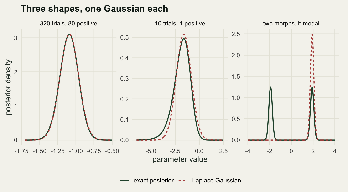
The first two panels are on the log-odds scale and the third on the separation scale. The left panel is what the approximation is for: 320 trials, 80 of them positive, and the two curves lie on top of each other. The middle panel is the same model with ten trials and one positive, and the mismatch is not subtle once you look at the left tail, where the exact posterior runs a long way towards minus infinity and the Gaussian stops. The right panel is the failure no sample size fixes: adding measurements sharpens both humps and leaves the approximation covering one of them.
Failure three: a boundary, where the answer is the wrong object
Skew and multimodality give a wrong answer to a well posed question. A variance component at the boundary is different in kind, and much more common in practice.
Take a balanced one-way random-effects design: eight sites, four measurements at each, a between-site standard deviation that is genuinely small, and residual variance one. The marginal likelihood is available in closed form because the covariance matrix has only two distinct eigenvalues, so we can profile the residual variance out and look at the profile in the between-site standard deviation alone. How often does it have an interior maximum?
sim_oneway <- function(K, m, s2u, s2e) {
  uu <- rnorm(K, 0, sqrt(s2u))
  yy <- rep(uu, each = m) + rnorm(K * m, 0, sqrt(s2e))
  yb <- as.vector(tapply(yy, rep(seq_len(K), each = m), mean))
  list(SSW = sum((yy - rep(yb, each = m))^2),
       SSB = m * sum((yb - mean(yy))^2), K = K, m = m)
}

nll_su <- function(su, dd) {
  optimise(function(le) {
    s2e <- exp(le)
    lam <- s2e + dd$m * su^2
    0.5 * (dd$K * log(lam) + dd$K * (dd$m - 1) * log(s2e) +
             dd$SSW / s2e + dd$SSB / lam)
  }, c(-6, 4), tol = 1e-10)$objective
}

set.seed(20260805)
K_g <- 8
m_g <- 4
su_true <- sqrt(0.05)
n_sets <- 300
sets <- lapply(seq_len(n_sets), function(i) sim_oneway(K_g, m_g, su_true^2, 1))
grad0 <- vapply(sets, function(dd) (nll_su(1e-4, dd) - nll_su(0, dd)) / 1e-4,
                numeric(1))
frac_edge <- mean(grad0 > 0)
print(round(c(n_groups = K_g, per_group = m_g, sigma_u_true = su_true,
              n_datasets = n_sets, percent_mode_at_zero = 100 * frac_edge), 4))
n_groups per_group sigma_u_true
8.0000 4.0000 0.2236
n_datasets percent_mode_at_zero
300.0000 47.6667 i_edge <- which(grad0 > 0)[1]
i_int <- which(grad0 < 0)[1]
mode_int <- optimise(function(s) nll_su(s, sets[[i_int]]), c(0, 3),
tol = 1e-10)$minimum
h2 <- 1e-3
curv_edge <- (nll_su(2 * h2, sets[[i_edge]]) - 2 * nll_su(h2, sets[[i_edge]]) +
nll_su(0, sets[[i_edge]])) / h2^2
stop_a <- optim(log(0.5), function(l) nll_su(exp(l), sets[[i_edge]]),
method = "BFGS")
stop_b <- optim(log(0.05), function(l) nll_su(exp(l), sets[[i_edge]]),
method = "BFGS")
print(round(c(interior_mode = mode_int, boundary_curvature = curv_edge,
implied_sd = 1 / sqrt(curv_edge),
implied_mass_below_zero = pnorm(0, 0, 1 / sqrt(curv_edge))), 5)) interior_mode boundary_curvature implied_sd
0.19982 3.51479 0.53340
implied_mass_below_zero
0.50000 print(c(optim_start_a = 0.5, optim_start_b = 0.05))optim_start_a optim_start_b
0.50 0.05 print(signif(c(log_scale_stop_from_half = exp(stop_a$par)), 4))log_scale_stop_from_half
0.006734 print(signif(c(log_scale_stop_from_small = exp(stop_b$par)), 4))log_scale_stop_from_small
0.005059 su_seq <- seq(0, 0.9, length.out = 121)
prof_edge <- -vapply(su_seq, nll_su, numeric(1), dd = sets[[i_edge]])
prof_int <- -vapply(su_seq, nll_su, numeric(1), dd = sets[[i_int]])
bd <- rbind(data.frame(su = su_seq, lp = prof_int - max(prof_int),
panel = "interior mode"),
data.frame(su = su_seq, lp = prof_edge - max(prof_edge),
panel = "mode at the boundary"))
pts <- data.frame(su = c(mode_int, 0), lp = c(0, 0),
panel = c("interior mode", "mode at the boundary"))
ggplot(bd, aes(su, lp)) +
geom_line(colour = te_pal$forest, linewidth = 0.9) +
geom_point(data = pts, colour = te_pal$clay, size = 3) +
facet_wrap(~panel, nrow = 1) +
labs(x = "between-group standard deviation", y = "profile log likelihood",
title = "Two datasets, one generating process") +
theme_te() +
theme(legend.position = "none", plot.margin = margin(8, 14, 4, 8))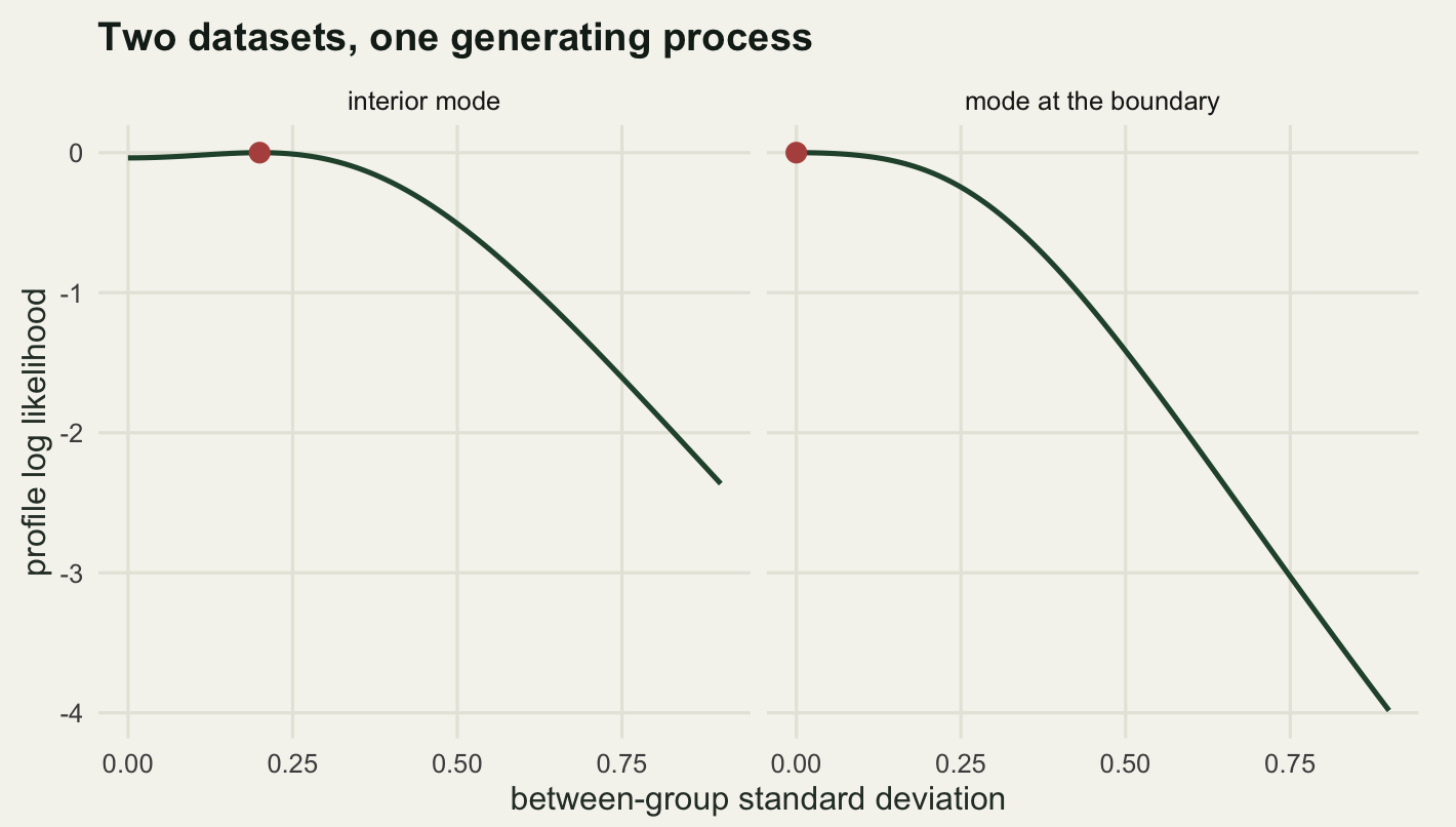
Out of 300 datasets simulated with a true between-site standard deviation of 0.2236, 47.6667 per cent had their maximum exactly at zero. Eight sites with four measurements each is an ordinary small ecological design, and roughly half the time the likelihood surface has no interior mode in the variance component.
The right-hand panel shows what that looks like. The profile is flat for a short distance and then falls, so there is no curvature at a peak to measure. What makes this dangerous is that the code does not stop. The numerical second derivative at the constrained optimum comes out as 3.51479, a positive number, so the Laplace machinery happily inverts it and reports a standard deviation of 0.5334 around a point estimate of zero. That Gaussian puts 0.5 of its mass on negative variance. It is not a small error in a good answer. It is a well formed answer to a question nobody asked.
Reparametrising does not save you. Moving to \(\log \sigma_u\), the standard trick for keeping a variance positive, sends the maximum to minus infinity, and optim stops wherever its tolerance runs out: 0.006734 starting from 0.5 and 0.005059 starting from 0.05. Two runs of the same code on the same data, stopping in different places, and neither a mode. Any standard error there reports the optimiser’s stopping rule.
The right response is not a better approximation. It is to notice, before fitting anything, that a variance component estimated from eight groups has a good chance of sitting on the boundary, and to handle it with a prior that keeps it away or an interval method that does not assume an interior maximum.
The payoff: integrating random effects away
None of this would matter if the approximation were not doing real work, and the real work is the inner integral of a mixed model. A Poisson generalised linear mixed model with a random intercept per group has a likelihood that integrates over every random effect, which is what lme4 approximates with Laplace by default and what glmmTMB does with automatic differentiation underneath.
The model is six transects with a random intercept each, counts at every visit, and two parameters: the overall log mean and the between-transect standard deviation. The design is nested, so the integral factorises into one one-dimensional integral per group, and a dense grid on each is a brute-force check. The Laplace route solves for the inner mode of each group by Newton’s method, a handful of steps each.
sim_glmm <- function(K, m, b0, su, seed) {
  set.seed(seed)
  uu <- rnorm(K, 0, su)
  yy <- rpois(K * m, exp(b0 + rep(uu, each = m)))
  list(S = as.vector(tapply(yy, rep(seq_len(K), each = m), sum)),
       K = K, m = m, lgam = sum(lgamma(yy + 1)), y = yy)
}

work <- new.env()
work$newton <- 0L
work$dens <- 0L

ll_laplace <- function(par, dd) {
  b0 <- par[1]
  su <- exp(par[2])
  tot <- 0
  for (j in seq_len(dd$K)) {
    sj <- dd$S[j]
    uu <- max(min(log(max(sj, 0.5) / dd$m) - b0, 5), -5)
    for (it in 1:50) {
      g1 <- sj - dd$m * exp(b0 + uu) - uu / su^2
      g2 <- -dd$m * exp(b0 + uu) - 1 / su^2
      step <- max(min(g1 / g2, 1), -1)
      uu <- uu - step
      work$newton <- work$newton + 1L
      if (abs(step) < 1e-11) break
    }
    tot <- tot + sj * (b0 + uu) - dd$m * exp(b0 + uu) - uu^2 / (2 * su^2) -
      log(su) - 0.5 * log(dd$m * exp(b0 + uu) + 1 / su^2)
  }
  tot - dd$lgam
}

ll_grid <- function(par, dd, ng = 4001) {
  b0 <- par[1]
  su <- exp(par[2])
  tot <- 0
  ug <- seq(-9 * su, 9 * su, length.out = ng)
  wdt <- diff(ug)[1]
  for (j in seq_len(dd$K)) {
    lg <- dd$S[j] * (b0 + ug) - dd$m * exp(b0 + ug) +
      dnorm(ug, 0, su, log = TRUE)
    mxx <- max(lg)
    work$dens <- work$dens + ng
    tot <- tot + mxx + log(sum(exp(lg - mxx)) * wdt)
  }
  tot - dd$lgam
}

compare_glmm <- function(K, m, b0, su, seed) {
  dd <- sim_glmm(K, m, b0, su, seed)
  work$newton <- 0L
  work$dens <- 0L
  start <- c(log(mean(dd$S / dd$m)), log(0.5))
  fl <- optim(start, function(p) -ll_laplace(p, dd), method = "BFGS",
              control = list(reltol = 1e-12))
  n_newton <- work$newton
  fq <- optim(start, function(p) -ll_grid(p, dd), method = "BFGS",
              control = list(reltol = 1e-12))
  data.frame(groups = K, per_group = m, mean_count = mean(dd$y),
             b0_lap = fl$par[1], b0_grid = fq$par[1],
             sigma_lap = exp(fl$par[2]), sigma_grid = exp(fq$par[2]),
             ll_lap = -fl$value, ll_grid = -fq$value,
             newton_steps = n_newton, grid_densities = work$dens)
}

gl <- rbind(compare_glmm(6, 8, log(3), 0.6, 20260802),
            compare_glmm(6, 4, log(1.5), 0.7, 20260805))
gl$sigma_pct_err <- 100 * (gl$sigma_lap - gl$sigma_grid) / gl$sigma_grid
gl$ll_err <- gl$ll_lap - gl$ll_grid
gl$work_ratio <- gl$grid_densities / gl$newton_steps
print(round(gl[, c("groups", "per_group", "mean_count", "b0_lap", "b0_grid",
                   "sigma_lap", "sigma_grid")], 4))
groups per_group mean_count b0_lap b0_grid sigma_lap sigma_grid
1 6 8 4.0625 1.3173 1.3172 0.4116 0.4122
2 6 4 2.0417 0.4280 0.4265 0.8471 0.8542print(round(gl[, c("ll_lap", "ll_grid", "ll_err", "sigma_pct_err")], 6)) ll_lap ll_grid ll_err sigma_pct_err
1 -104.30962 -104.30327 -0.006358 -0.155687
2 -39.34588 -39.32724 -0.018635 -0.824776print(round(c(sigma_pct_err_1 = gl$sigma_pct_err[1],
sigma_pct_err_2 = gl$sigma_pct_err[2],
sigma_abs_pct_err_1 = abs(gl$sigma_pct_err[1])), 4)) sigma_pct_err_1 sigma_pct_err_2 sigma_abs_pct_err_1
-0.1557 -0.8248 0.1557 print(round(c(grid_points_per_group = 4001,
newton_steps_1 = gl$newton_steps[1],
grid_densities_1 = gl$grid_densities[1],
work_ratio_1 = gl$work_ratio[1],
work_ratio_2 = gl$work_ratio[2]), 1))grid_points_per_group newton_steps_1 grid_densities_1
4001.0 1531.0 1368342.0
work_ratio_1 work_ratio_2
893.8 744.9 The first design has 6 transects with 8 visits each and a mean count of 4.0625. The Laplace-based fit returns a log mean of 1.3173 and a between-transect standard deviation of 0.4116. The grid-based fit, integrating the same likelihood with 4001 points per group per evaluation, returns 1.3172 and 0.4122. The maximised log likelihoods differ by -0.006358 and the standard deviation by -0.1557 per cent.
That is better than the folklore suggests. This is the regime where Laplace is supposed to struggle, and the numbers above show it matching the brute-force integration closely on the log mean, on the standard deviation and on the log likelihood. Halving the visits and dropping the mean count to 2.0417, in the second row, widens the gap to -0.8248 per cent on the standard deviation and -0.018635 on the log likelihood, which is the expected direction and still small next to the sampling uncertainty in six groups.
The cost difference is what makes the method worth having. Counting the work rather than timing it: the Laplace fit took 1531 inner Newton updates in total, and the grid fit evaluated the group integrand 1368342 times, a ratio of 893.8 to one. In the second design the ratio was 744.9 to one. Scale up to a real dataset with crossed random effects and the grid stops being an option, because the integral no longer factorises and its dimension is the number of random effects. The Laplace cost grows with one sparse linear solve.
Both errors above have the same sign: the Laplace fit puts the between-group standard deviation below the grid value in both designs. A downward bias in the variance component is the known behaviour of the approximation here, and it is why software that offers adaptive quadrature offers it for the small-cluster case in particular.
What to take away
The approximation is three lines once you have the mode and the Hessian, and it earns its place. It reproduced an exact marginal likelihood to 3.18e-12 in the conjugate case, tracked the beta-binomial marginal likelihood at a clean \(O(1/n)\) rate with a fitted exponent of -0.982, and came within 0.1557 per cent of a brute-force integration of a Poisson mixed model on the variance component while doing 893.8 times less arithmetic.
Two of the measurements went against what I expected to find. The posterior mean does not converge faster than the tail quantile: the fitted exponents were -0.977 and -0.923, near enough the same, and what separates them is a constant near 1.887 that does not shrink. Only the posterior standard deviation converges genuinely faster, at -1.475. And the scale with the least skew was not the scale with the best interval: the cube root scale had a skewness of -0.1672 against 0.3076 for the arcsine root, and an endpoint error three times larger, because straightening the skew widened the interval by a factor of 1.1981 and shifted its centre by 0.0397.
The three failures rank by how likely they are to reach a published table. Skew is the mildest: the interval is misplaced by 0.3021 of its own width while its size is nearly right, and a change of scale removes most of that. Multimodality is quiet and exact, half the mass missed and a Bayes factor out by 0.6931 log units. A variance component on the boundary is the one to watch for, because it happened in 47.6667 per cent of 300 datasets from an ordinary eight-group design, and the machinery returns a standard deviation of 0.5334 around zero without a warning.
The honest limit follows from what the method is. It is a statement about the curvature of the log posterior at one point, so nothing inside it can tell you that the posterior has a second mode, a boundary maximum or a tail the Gaussian cannot reach; every diagnosis in this post came from outside, from an exact formula or a dense grid, and in a problem where neither exists the check has to come from a sampler run once at the start. Fitting a Gaussian and reading off its quantiles is fast and usually right, and the cases where it is wrong are the cases where nothing in the output looks unusual.
References
Tierney L, Kadane JB 1986 Journal of the American Statistical Association 81(393):82-86 (10.1080/01621459.1986.10478240)
Kass RE, Raftery AE 1995 Journal of the American Statistical Association 90(430):773-795 (10.1080/01621459.1995.10476572)
Breslow NE, Clayton DG 1993 Journal of the American Statistical Association 88(421):9-25 (10.1080/01621459.1993.10594284)
Rue H, Martino S, Chopin N 2009 Journal of the Royal Statistical Society Series B 71(2):319-392 (10.1111/j.1467-9868.2008.00700.x)
Bates D, Maechler M, Bolker B, Walker S 2015 Journal of Statistical Software 67(1):1-48 (10.18637/jss.v067.i01)
Bolker BM, Brooks ME, Clark CJ, Geange SW, Poulsen JR, Stevens MHH, White JSS 2009 Trends in Ecology and Evolution 24(3):127-135 (10.1016/j.tree.2008.10.008)
Gelman A, Carlin JB, Stern HS, Dunson DB, Vehtari A, Rubin DB 2013 Bayesian Data Analysis, third edition (ISBN 978-1-4398-4095-5)