library(ggplot2)

te_pal <- list(forest = "#275139", green = "#2f8f63", sage = "#93a87f",
               clay = "#b5534e", gold = "#cda23f", line = "#dad9ca",
               ink = "#16241d", paper = "#f5f4ee")

theme_te <- function() {
  theme_minimal(base_size = 12) +
    theme(panel.grid.minor = element_blank(),
          panel.grid.major = element_line(colour = "#e7e6dc"),
          plot.background = element_rect(fill = "#f5f4ee", colour = NA),
          panel.background = element_rect(fill = "#f5f4ee", colour = NA),
          plot.title = element_text(face = "bold", colour = te_pal$ink),
          axis.title = element_text(colour = "#2c3a31"),
          axis.text = element_text(colour = "#2c3a31"))
}Slice sampling from scratch
R
MCMC
Bayesian statistics
ecology tutorial
Build a slice sampler in base R on an ecological count posterior, and measure the claim that it needs no tuning against a random-walk sampler that does.
A carabid survey in an arable mosaic: twelve field margins, six pitfall traps in each, emptied fortnightly from May to the end of August. Traps get trampled, flooded and mown over, so the margins did not all deliver the same amount of trapping, and the season’s catch of one common ground beetle is recorded as a count per margin alongside the trap-nights that produced it. The first question is the catch rate per hundred trap-nights, with an interval that respects the fact that twelve margins is not many. That posterior is available in closed form, which is what makes it useful here: this post builds a slice sampler in base R, points it at that posterior, checks it against the answer nobody had to sample for, and then points the same code, unchanged, at two posteriors that are genuinely unpleasant.
The reason for writing it is a gap in the sampler cluster on this blog. Metropolis-Hastings from scratch devotes a section to tuning the proposal width, and the sales pitch for slice sampling is that it does not have one. That pitch is half true: the slice sampler does have a width, it just matters far less, and this post puts a number on far less rather than repeating the claim. Gibbs sampling with conjugate updates needs every full conditional to be a standard distribution, and the commonest real use of slice sampling is to replace the one that is not. Hamiltonian Monte Carlo from scratch counts cost in gradient evaluations rather than iterations, and the same currency is used throughout here so the three posts can be read against each other. MCMC convergence diagnostics from scratch builds the effective sample size estimator every efficiency figure below depends on, used here without being re-explained. And reparameterisation and Neal’s funnel already owns the funnel geometry, so the awkward targets here are a different pair: a posterior with no finite variance, and two coefficients wound tightly around each other.
The survey, and a posterior that needs no sampler
Counts with unequal effort are the plainest model in this corner of ecology. The catch at margin \(i\) is Poisson with mean \(\lambda E_i\), where \(E_i\) is the trapping effort in hundreds of trap-nights, and a gamma prior on \(\lambda\) makes the posterior another gamma: shape equal to the prior shape plus the total catch, rate equal to the prior rate plus the total effort. The sampler works on \(\theta = \log \lambda\), because the log rate lives on the whole real line and a sampler that has to notice a boundary is a different problem. After the change of variables the log density is \(a\theta - b e^{\theta}\) up to a constant, and its exact quantiles are the logs of the gamma quantiles.
set.seed(20260803)
n_site <- 12
trap_nights <- round(runif(n_site, 60, 180) / 2) * 2
effort <- trap_nights / 100
lam_true <- 8
y_cnt <- rpois(n_site, lam_true * effort)

a0 <- 2
b0 <- 0.5
a_post <- a0 + sum(y_cnt)
b_post <- b0 + sum(effort)
sd_exact <- sqrt(trigamma(a_post))
mean_exact <- digamma(a_post) - log(b_post)

lp_rate <- function(th) a_post * th - b_post * exp(th)

print(rbind(trap_nights = trap_nights, catch = y_cnt))
[,1] [,2] [,3] [,4] [,5] [,6] [,7] [,8] [,9] [,10] [,11] [,12]
trap_nights 74 106 82 174 154 106 104 130 140 84 138 68
catch 4 15 13 14 9 11 6 11 10 7 15 10print(round(c(margins = n_site, total_catch = sum(y_cnt),
total_effort = sum(effort), post_shape = a_post,
post_rate = b_post, post_mean_rate = a_post / b_post), 3)) margins total_catch total_effort post_shape post_rate
12.000 125.000 13.600 127.000 14.100
post_mean_rate
9.007 print(round(c(post_mean_lograte = mean_exact, post_sd_lograte = sd_exact,
exact_q025 = log(qgamma(0.025, a_post, rate = b_post)),
exact_q975 = log(qgamma(0.975, a_post, rate = b_post))), 5))post_mean_lograte post_sd_lograte exact_q025 exact_q975
2.19407 0.08891 2.01608 2.36459 The twelve margins delivered 125 beetles over 1360 trap-nights, the least productive returning 4 and the most productive 15. The posterior mean rate is 9.0071 beetles per hundred trap-nights, and on the log scale the posterior has mean 2.19407 and standard deviation 0.08891. Every sampler setting below is quoted in multiples of that standard deviation, because a setting only means anything relative to the width of the target.
Sampling uniformly under the curve
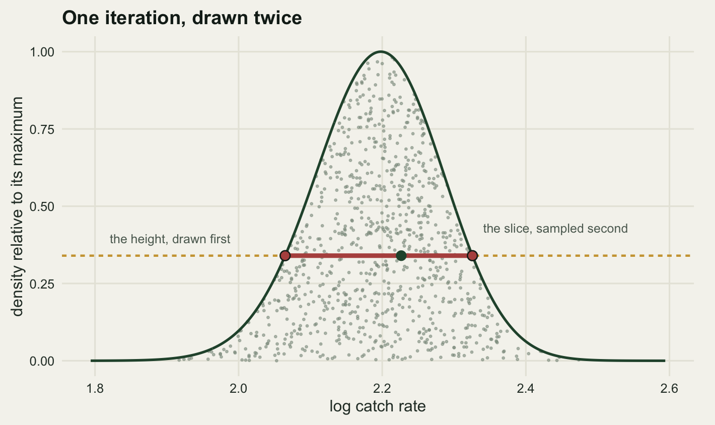
The idea is one sentence long. Take the target density \(f\), and instead of sampling \(\theta\) from it, sample a point \((\theta, y)\) uniformly from the two-dimensional region under the curve; the horizontal coordinate of such a point has exactly the density \(f\), because the vertical extent of the region above any \(\theta\) is \(f(\theta)\). Throw the height away and what is left is a draw from the target.
Sampling uniformly from that region is not obviously easier than the original problem. What makes it work is that the uniform distribution on it has two trivial conditionals. Given \(\theta\), the height is uniform on \((0, f(\theta))\). Given the height \(y\), the position is uniform on the slice \(S = \{\theta : f(\theta) > y\}\), the set of positions whose density clears that height. Alternating those two draws is a Gibbs sampler on the joint distribution, so the joint is invariant, so its horizontal marginal is invariant, and that marginal is the target. Nothing is accepted or rejected and no proposal distribution appears anywhere in the argument. The construction is due to Neal (2003); the same auxiliary-variable trick appears in Higdon (1998) and in Damlen, Wakefield and Walker (1999), and Roberts and Rosenthal (1999) supply the convergence theory for the resulting chains.
The argument has a consequence worth checking later. If the pairs are uniform under the curve then the heights are not uniform: the marginal density of the height is proportional to the length of the slice at that height, and slices are long near the bottom of the curve and short near the top. That length can be found by root-finding here, so the whole predicted distribution of heights is available before any chain is run.
th_mode <- log(a_post / b_post)
lf_max <- lp_rate(th_mode)

slice_len <- function(rel_h) {
  tgt <- log(rel_h) + lf_max
  lo <- uniroot(function(z) lp_rate(z) - tgt, c(th_mode - 20, th_mode),
                tol = 1e-12)$root
  hi <- uniroot(function(z) lp_rate(z) - tgt, c(th_mode, th_mode + 20),
                tol = 1e-12)$root
  hi - lo
}

h_grid <- seq(1e-6, 1 - 1e-9, length.out = 3001)
len_grid <- vapply(h_grid, slice_len, numeric(1))
h_cdf <- c(0, cumsum((len_grid[-1] + len_grid[-length(len_grid)]) / 2 * diff(h_grid)))
h_cdf <- h_cdf / max(h_cdf)
probs_h <- c(0.1, 0.25, 0.5, 0.75, 0.9)
h_theory <- approx(h_cdf, h_grid, xout = probs_h)$y
print(round(c(mode = th_mode, length_at_tenth = slice_len(0.1) / sd_exact,
              length_at_nine_tenths = slice_len(0.9) / sd_exact), 4))
mode length_at_tenth length_at_nine_tenths
2.1980 4.2878 0.9163 The slice at a tenth of the maximum density is 4.288 posterior standard deviations long and the slice at nine tenths is 0.916, so low heights should be drawn far more often than high ones, with a predicted median relative height of 0.30616.
The hard part is finding the slice
Everything above assumed the slice could be handed over on request. Root-finding does that here, but it needs a unimodal target and a bracket, and neither survives contact with a real model. The working algorithm never computes the slice. It constructs an interval containing part of it, then shrinks that interval towards the current point until a candidate lands inside.
Stepping out builds the interval: place an interval of width \(w\) at random around the current position, so the current position sits at a uniformly distributed place inside it, then extend it in steps of \(w\) on whichever side still has an endpoint under the curve until both endpoints are above the height. Shrinkage does the sampling: draw a candidate uniformly from the interval, accept it if its density clears the height, and otherwise make the rejected candidate the new endpoint on whichever side it fell and draw again from the smaller interval.
The shrinkage step is what keeps the chain valid, and the reason is worth stating plainly because the shortcut is so tempting. Suppose you skipped it and simply resampled candidates from a fixed interval of width \(w\) centred on the current point until one landed in the slice. That is ordinary rejection sampling and it looks harmless. It is not reversible: the probability of moving from \(\theta\) to \(\theta'\) involves the length of the slice inside the interval around \(\theta\), the probability of moving back involves the length inside the interval around \(\theta'\), and those differ whenever the target is not flat. Shrinking one interval that was fixed before any candidate was drawn, rather than recentring it every time, is what makes the two directions match.
slice_step <- function(x0, lf0, logf, w, m_lim) {
  ev <- 0L
  logy <- lf0 - rexp(1)                       # log of a uniform height under f
  lo <- x0 - w * runif(1); hi <- lo + w       # interval placed at random
  j_left <- floor(m_lim * runif(1))           # split of the step-out budget
  k_right <- (m_lim - 1) - j_left
  while (j_left > 0) {                        # stepping out
    ev <- ev + 1L
    if (logf(lo) <= logy) break
    lo <- lo - w; j_left <- j_left - 1
  }
  while (k_right > 0) {
    ev <- ev + 1L
    if (logf(hi) <= logy) break
    hi <- hi + w; k_right <- k_right - 1
  }
  repeat {                                    # shrinkage
    x1 <- lo + runif(1) * (hi - lo)
    lf1 <- logf(x1); ev <- ev + 1L
    if (lf1 > logy) break
    if (x1 < x0) lo <- x1 else hi <- x1
  }
  c(x1, lf1, ev)
}

slice_chain <- function(x0, logf, w, n_iter, m_lim = 1e6, seed = 1) {
  set.seed(seed)
  out <- numeric(n_iter); x <- x0; lf <- logf(x); ev <- 0
  for (i in seq_len(n_iter)) {
    r <- slice_step(x, lf, logf, w, m_lim)
    x <- r[1]; lf <- r[2]; ev <- ev + r[3]; out[i] <- x
  }
  list(draws = out, evals = ev + 1, per_iter = ev / n_iter)
}

rw_chain <- function(x0, logf, prop_sd, n_iter, seed = 1) {
  set.seed(seed)
  out <- numeric(n_iter); x <- x0; lf <- logf(x); acc <- 0L
  jump <- rnorm(n_iter, 0, prop_sd); logu <- log(runif(n_iter))
  for (i in seq_len(n_iter)) {
    xp <- x + jump[i]; lfp <- logf(xp)
    if (logu[i] < lfp - lf) { x <- xp; lf <- lfp; acc <- acc + 1L }
    out[i] <- x
  }
  list(draws = out, evals = n_iter + 1, accept = acc / n_iter)
}
One note on the step-out budget. Setting m_lim to a finite value caps the number of extensions, and the cap is split at random between the two sides rather than applied to each, because a deterministic cap would break the symmetry the reversibility argument relies on (Neal 2003). It is high enough here to be effectively unlimited, and a later section measures what happens when it is not.
The claim that the shortcut is wrong can be measured rather than asserted. Both samplers below draw the same height in the same way; the only difference is that one shrinks a fixed interval and the other keeps redrawing from an interval recentred on the current point.
naive_chain <- function(x0, logf, w, n_iter, seed = 1) {
  set.seed(seed)
  out <- numeric(n_iter); x <- x0; lf <- logf(x); ev <- 0
  for (i in seq_len(n_iter)) {
    logy <- lf - rexp(1)
    repeat {                        # rejection sampling on a recentred interval
      xp <- x + w * (runif(1) - 0.5)
      lfp <- logf(xp); ev <- ev + 1
      if (lfp > logy) break
    }
    x <- xp; lf <- lfp; out[i] <- x
  }
  list(draws = out, evals = ev, per_iter = ev / n_iter)
}

n_rep_b <- 8; n_it_b <- 20000
w_bias <- c(0.3, 1, 10) * sd_exact
bias_tab <- data.frame(w_over_sd = w_bias / sd_exact, naive_sd = NA_real_,
                       naive_mcse = NA_real_, good_sd = NA_real_)
for (k in seq_along(w_bias)) {
  s_naive <- s_good <- numeric(n_rep_b)
  for (r in seq_len(n_rep_b)) {
    s_naive[r] <- sd(naive_chain(mean_exact, lp_rate, w_bias[k], n_it_b,
                                 seed = 1000 * r + 7)$draws)
    s_good[r] <- sd(slice_chain(mean_exact, lp_rate, w_bias[k], n_it_b,
                                seed = 2000 * r + 7)$draws)
  }
  bias_tab$naive_sd[k] <- mean(s_naive)
  bias_tab$naive_mcse[k] <- sd(s_naive) / sqrt(n_rep_b)
  bias_tab$good_sd[k] <- mean(s_good)
}
bias_tab$naive_ratio <- bias_tab$naive_sd / sd_exact
bias_tab$good_ratio <- bias_tab$good_sd / sd_exact
bias_tab$in_mcse <- (bias_tab$naive_sd - sd_exact) / bias_tab$naive_mcse
k_bias <- which.max(abs(bias_tab$in_mcse))
print(round(bias_tab, 5))
w_over_sd naive_sd naive_mcse good_sd naive_ratio good_ratio in_mcse
1 0.3 0.07170 0.00122 0.08871 0.80642 0.99779 -14.11932
2 1.0 0.07403 0.00052 0.08877 0.83268 0.99846 -28.79371
3 10.0 0.08818 0.00025 0.08905 0.99174 1.00160 -2.96382print(round(c(exact_sd = sd_exact, worst_row = k_bias,
worst_shortfall_pct = 100 * (1 - bias_tab$naive_ratio[k_bias]),
worst_in_mcse = bias_tab$in_mcse[k_bias],
widest_naive_ratio = bias_tab$naive_ratio[nrow(bias_tab)]), 4)) exact_sd worst_row worst_shortfall_pct worst_in_mcse
0.0889 2.0000 16.7317 -28.7937
widest_naive_ratio
0.9917 At the width where the bias stands out most clearly from the chain-to-chain noise, 1 times the posterior standard deviation, the naive sampler returns a posterior standard deviation of 0.07403 against the exact 0.08891, which is 83.27 per cent of the truth and 28.8 Monte Carlo standard errors away from it. The correct sampler at the same width returns 0.08877, or 99.85 per cent. The naive chain is not noisier; it is systematically too concentrated, which is the failure mode least likely to be noticed, because a too-narrow posterior looks like a well-behaved one.
The bias fades only when the interval is wide enough to swallow the whole slice most of the time: at 10 posterior standard deviations it is down to 0.83 per cent. That is the trap. The shortcut is exactly correct in the limit where it is also pointless, and wrong across the whole range of widths anyone would choose on purpose.
Checking against the exact answer
Eight independent chains, each started from the posterior mean, with the quantile estimates averaged across chains and their spread across chains used as the Monte Carlo standard error. The heights get checked in the same pass: given a stationary draw, the height is uniform below the density there, so the pairs can be rebuilt from the stored chain and held against the prediction made two sections ago.
n_chain <- 8; n_it_chk <- 20000
probs_chk <- c(0.025, 0.25, 0.5, 0.75, 0.975)
q_mat <- matrix(NA_real_, n_chain, length(probs_chk))
h_mat <- matrix(NA_real_, n_chain, length(probs_h))
mean_ch <- sd_ch <- numeric(n_chain)
set.seed(4242)
for (r in seq_len(n_chain)) {
  ch <- slice_chain(mean_exact, lp_rate, 3 * sd_exact, n_it_chk, seed = 8100 + r)
  q_mat[r, ] <- quantile(ch$draws, probs_chk)
  mean_ch[r] <- mean(ch$draws); sd_ch[r] <- sd(ch$draws)
  h_mat[r, ] <- quantile(exp(lp_rate(ch$draws) - lf_max - rexp(n_it_chk)), probs_h)
}
chk <- data.frame(prob = probs_chk,
                  exact = log(qgamma(probs_chk, a_post, rate = b_post)),
                  sampled = colMeans(q_mat),
                  mcse = apply(q_mat, 2, sd) / sqrt(n_chain))
chk$error <- chk$sampled - chk$exact
chk$in_mcse <- chk$error / chk$mcse
print(round(chk, 6))
prob exact sampled mcse error in_mcse
1 0.025 2.016077 2.016398 0.000533 0.000322 0.603069
2 0.250 2.134865 2.134902 0.000309 0.000037 0.120305
3 0.500 2.195385 2.195144 0.000232 -0.000242 -1.042289
4 0.750 2.254710 2.254589 0.000351 -0.000121 -0.345712
5 0.975 2.364588 2.363859 0.000559 -0.000729 -1.303023print(round(c(mean_sampled = mean(mean_ch), mean_exact = mean_exact,
mean_mcse = sd(mean_ch) / sqrt(n_chain),
sd_sampled = mean(sd_ch), sd_exact = sd_exact,
worst_quantile_in_mcse = max(abs(chk$in_mcse))), 5)) mean_sampled mean_exact mean_mcse
2.19402 2.19407 0.00015
sd_sampled sd_exact worst_quantile_in_mcse
0.08866 0.08891 1.30302 h_sampled <- colMeans(h_mat)
h_mcse <- apply(h_mat, 2, sd) / sqrt(n_chain)
print(round(rbind(prob = probs_h, predicted = h_theory, sampled = h_sampled,
mcse = h_mcse, in_mcse = (h_sampled - h_theory) / h_mcse), 5)) [,1] [,2] [,3] [,4] [,5]
prob 0.10000 0.25000 0.50000 0.75000 0.90000
predicted 0.04380 0.12803 0.30616 0.54521 0.74651
sampled 0.04415 0.12832 0.30743 0.54546 0.74747
mcse 0.00047 0.00060 0.00102 0.00119 0.00086
in_mcse 0.73557 0.47894 1.24294 0.20877 1.10816The posterior mean comes back as 2.19402 against an exact 2.19407, a discrepancy of 0.35 Monte Carlo standard errors. All five quantiles land within 1.30 standard errors of the exact gamma values, the worst being the 97.5 per cent point at 2.36386 against 2.36459. The heights agree with the prediction too, the largest departure over their five quantiles being 1.24 Monte Carlo standard errors, so the auxiliary variable is distributed the way the invariance argument says it has to be. Nothing was tuned to get any of this: the width was set to three posterior standard deviations because it was a round number, which the next section says is roughly why it did not matter.
Sweeping the dial
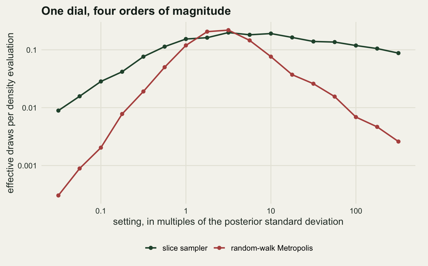
Here is the comparison the post exists for. Both samplers get the same evaluation budget at every setting, the slice sampler running a short pilot first so its iteration count can be chosen to spend that budget. The same grid of settings, four orders of magnitude wide, serves as the slice width and as the Metropolis proposal standard deviation.
The effective sample size estimator is the one the diagnostics post builds, with Geyer’s initial positive sequence to decide where to stop summing autocorrelations. Nothing here uses the rank-normalised and folded refinements of Vehtari et al (2021), which is the version worth reaching for on a real posterior with heavy tails or a badly behaved variance.
autocov <- function(x) {
  n <- length(x); x <- x - mean(x)
  n2 <- 2^ceiling(log2(2 * n)); fx <- fft(c(x, rep(0, n2 - n)))
  Re(fft(fx * Conj(fx), inverse = TRUE))[seq_len(n)] / (n2 * n)
}

ess_series <- function(x) {
  n <- length(x); gam <- autocov(x)
  if (gam[1] <= 0) return(NA_real_)
  rho <- gam / gam[1]; k <- floor((n - 2) / 2)
  paired <- rho[2 * seq_len(k)] + rho[2 * seq_len(k) + 1]
  stop_at <- which(paired <= 0)
  m_stop <- if (length(stop_at)) stop_at[1] - 1L else k
  n / (1 + 2 * (if (m_stop >= 1) sum(paired[seq_len(m_stop)]) else 0))
}
budget <- 40000
mult_grid <- 10^seq(-1.5, 2.5, by = 0.25)
swp <- data.frame(mult = mult_grid, dial = mult_grid * sd_exact,
per_iter = NA_real_, slice = NA_real_,
accept = NA_real_, metrop = NA_real_)
for (i in seq_along(mult_grid)) {
pilot <- slice_chain(mean_exact, lp_rate, swp$dial[i], 200, seed = 300 + i)
n_it <- max(200, floor(budget / pilot$per_iter))
ch <- slice_chain(mean_exact, lp_rate, swp$dial[i], n_it, seed = 400 + i)
swp$per_iter[i] <- ch$per_iter
swp$slice[i] <- ess_series(ch$draws) / ch$evals
rw <- rw_chain(mean_exact, lp_rate, swp$dial[i], budget, seed = 500 + i)
swp$accept[i] <- rw$accept
swp$metrop[i] <- ess_series(rw$draws) / rw$evals
}
print(round(swp[seq(1, nrow(swp), by = 2), ], 5)) mult dial per_iter slice accept metrop
1 0.03162 0.00281 107.62887 0.00891 0.98582 0.00030
3 0.10000 0.00889 34.52911 0.02838 0.96667 0.00204
5 0.31623 0.02812 13.13143 0.07615 0.90358 0.01906
7 1.00000 0.08891 6.50772 0.15366 0.70328 0.11915
9 3.16228 0.28116 4.91002 0.19868 0.35640 0.21886
11 10.00000 0.88911 5.23735 0.19093 0.12430 0.07615
13 31.62278 2.81160 6.57125 0.13931 0.03900 0.02594
15 100.00000 8.89106 8.43047 0.11861 0.01158 0.00688
17 316.22777 28.11600 10.53968 0.08772 0.00432 0.00260sl_span <- max(swp$slice) / min(swp$slice)
mh_span <- max(swp$metrop) / min(swp$metrop)
print(round(c(slice_best = max(swp$slice), slice_worst = min(swp$slice),
slice_span = sl_span,
slice_best_at_mult = swp$mult[which.max(swp$slice)]), 5)) slice_best slice_worst slice_span slice_best_at_mult
0.19868 0.00891 22.29612 3.16228 print(round(c(metrop_best = max(swp$metrop), metrop_worst = min(swp$metrop),
metrop_span = mh_span,
metrop_best_at_mult = swp$mult[which.max(swp$metrop)],
metrop_best_accept = swp$accept[which.max(swp$metrop)]), 5)) metrop_best metrop_worst metrop_span metrop_best_at_mult
0.21886 0.00030 719.23650 3.16228
metrop_best_accept
0.35640 print(round(c(span_ratio = mh_span / sl_span,
peak_ratio = max(swp$slice) / max(swp$metrop)), 4))span_ratio peak_ratio
32.2584 0.9078 small_end <- swp$mult <= 0.32
big_end <- swp$mult >= 10
fit_small <- lm(swp$per_iter[small_end] ~ I(sd_exact / swp$dial[small_end]))
fit_big <- lm(swp$per_iter[big_end] ~ I(log2(swp$dial[big_end])))
print(round(c(evals_per_sd_over_w = unname(coef(fit_small)[2]),
small_end_r2 = summary(fit_small)$r.squared,
evals_per_doubling = unname(coef(fit_big)[2]),
big_end_r2 = summary(fit_big)$r.squared,
cheapest_per_iter = min(swp$per_iter),
cheapest_at_mult = swp$mult[which.min(swp$per_iter)]), 4))evals_per_sd_over_w small_end_r2 evals_per_doubling big_end_r2
3.3318 0.9998 1.0791 0.9885
cheapest_per_iter cheapest_at_mult
4.8603 5.6234 At its best setting the slice sampler delivers 0.1987 effective draws per density evaluation and the random walk delivers 0.2189, so at the top of each curve the slice sampler is 9.2 per cent behind. That goes against the folklore and it is the first thing to say: slice sampling does not buy peak efficiency, and a well-tuned random walk on a smooth one-dimensional posterior is hard to beat.
What it buys is everything either side of the peak. Across the four orders of magnitude swept, the slice sampler’s efficiency varies by a factor of 22.3 and the random walk’s by 719.2, a difference of 32.3 times in how much the setting matters. At the smallest setting the random walk returns 0.000304 effective draws per evaluation, or 0.139 per cent of its own best, against 4.49 per cent for the slice sampler. The slice curve is not flat, though, and its two tails have different shapes, which can be pinned down.
A width that is too small is punished linearly: each further factor by which \(w\) falls short of the posterior standard deviation costs about 3.33 more density evaluations per iteration, a straight line in the reciprocal of the width fitting the small end with an r-squared of 0.9998. A width that is too large is punished logarithmically, because shrinkage roughly halves the interval each time it fails: the cost grows by 1.08 evaluations per doubling, with an r-squared of 0.9885. That asymmetry is the practical rule the method rests on. From the cheapest iteration in the sweep, 4.86 evaluations at 5.62 posterior standard deviations, going a thousandfold too wide costs about ten evaluations per iteration and going a thousandfold too narrow costs several hundred. When in doubt, guess high.
A posterior with no finite variance
The pilot season of the same scheme ran three margins only. Treating the three log catch rates as normal with unknown mean and unknown variance under the standard reference prior (Gelman et al 2013) gives the marginal posterior for the mean that the Gibbs post derives: a Student t on the sample mean, scaled by the standard error, with degrees of freedom one less than the sample size. At three margins that is a t with two degrees of freedom, whose variance does not exist. Its quantiles do, which makes it an awkward target with a known answer. Mengersen and Tweedie (1996) showed that a symmetric random walk is not geometrically ergodic when the tails are heavier than exponential, and the practical symptom is a chain that wanders far out and then cannot get back, because from out there every proposal of a sensible size looks as good as staying put.
pilot_nights <- c(120, 96, 140)
pilot_y <- c(3, 11, 5)
pilot_lr <- log(pilot_y / (pilot_nights / 100))
n_pilot <- 3
m_pilot <- mean(pilot_lr)
sc_pilot <- sd(pilot_lr) / sqrt(n_pilot)
df_pilot <- n_pilot - 1
lp_heavy <- function(x) {
  -((df_pilot + 1) / 2) * log1p(((x - m_pilot) / sc_pilot)^2 / df_pilot)
}
q99 <- m_pilot + sc_pilot * qt(0.99, df_pilot)
print(round(c(pilot_log_rates = pilot_lr, centre = m_pilot, scale = sc_pilot,
              deg_freedom = df_pilot, exact_q99 = q99), 4))
pilot_log_rates1 pilot_log_rates2 pilot_log_rates3 centre
0.9163 2.4387 1.2730 1.5427
scale deg_freedom exact_q99
0.4597 2.0000 4.7443 budget_h <- 60000; n_rep_h <- 16; mult_h <- c(0.1, 1, 10, 100)
sl_draws <- mh_draws <- matrix(NA_real_, n_rep_h, length(mult_h))
heavy <- data.frame(mult = mult_h, sl_rmse = NA_real_, sl_bias = NA_real_,
sl_per_iter = NA_real_, mh_rmse = NA_real_,
mh_bias = NA_real_, mh_accept = NA_real_)
for (k in seq_along(mult_h)) {
dial <- mult_h[k] * sc_pilot; per_it <- numeric(n_rep_h); acc_r <- numeric(n_rep_h)
for (r in seq_len(n_rep_h)) {
pilot <- slice_chain(m_pilot, lp_heavy, dial, 300, seed = r)
ch <- slice_chain(m_pilot, lp_heavy, dial,
floor(budget_h / pilot$per_iter), seed = 5000 + r)
sl_draws[r, k] <- quantile(ch$draws, 0.99); per_it[r] <- ch$per_iter
rw <- rw_chain(m_pilot, lp_heavy, dial, budget_h, seed = 6000 + r)
mh_draws[r, k] <- quantile(rw$draws, 0.99); acc_r[r] <- rw$accept
}
heavy$sl_rmse[k] <- sqrt(mean((sl_draws[, k] - q99)^2))
heavy$sl_bias[k] <- mean(sl_draws[, k]) - q99; heavy$sl_per_iter[k] <- mean(per_it)
heavy$mh_rmse[k] <- sqrt(mean((mh_draws[, k] - q99)^2))
heavy$mh_bias[k] <- mean(mh_draws[, k]) - q99; heavy$mh_accept[k] <- mean(acc_r)
}
print(round(heavy, 4)) mult sl_rmse sl_bias sl_per_iter mh_rmse mh_bias mh_accept
1 0.1 0.6171 -0.0335 58.8547 1.3171 -1.0375 0.9715
2 1.0 0.2720 0.0027 8.9178 1.7561 0.8177 0.7453
3 10.0 0.2069 -0.0247 5.2509 0.2021 -0.0882 0.1900
4 100.0 0.2503 0.0000 7.9617 0.3785 0.1127 0.0224print(round(c(slice_rmse_span = max(heavy$sl_rmse) / min(heavy$sl_rmse),
metrop_rmse_span = max(heavy$mh_rmse) / min(heavy$mh_rmse),
metrop_best_at_mult = heavy$mult[which.min(heavy$mh_rmse)]), 4)) slice_rmse_span metrop_rmse_span metrop_best_at_mult
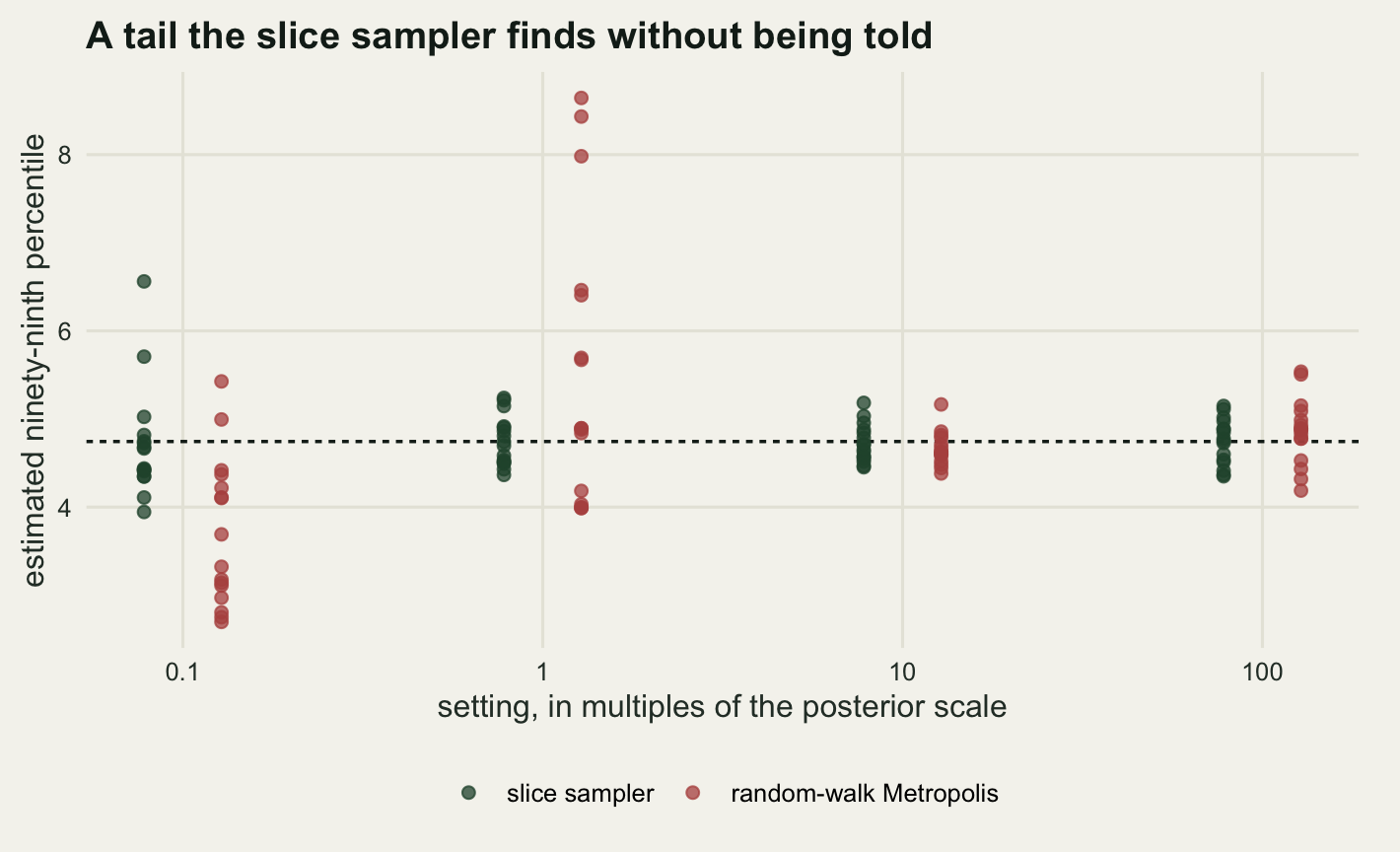
2.9831 8.6898 10.0000 The quantity estimated is the ninety-ninth percentile of the posterior, exactly 4.7443, and the error is the root mean squared deviation of that estimate over 16 independent chains. Across three orders of magnitude of the setting, the slice sampler’s error runs from 0.2069 to 0.6171, a span of 2.98; the random walk’s from 0.2021 to 1.7561, a span of 8.69.
Read the middle of that table before drawing the obvious conclusion, because it is not the obvious one. The best random walk in the sweep is as accurate as the best slice sampler: 0.2021 against 0.2069. But the setting that achieves it is 10 times the scale of the posterior bulk, accepting only 19 per cent of its proposals, and nothing about the target tells you to go there. The natural choice, a proposal matched to the bulk of the posterior, accepts 74.5 per cent of its moves, and its error is 1.7561, worse by a factor of 8.7. The slice sampler at that same natural setting is already at 0.272. The gain is not that slice sampling reaches somewhere Metropolis cannot; it is that it reaches it from the setting a reasonable person would pick.
The mechanism is stepping out. A chain far out in the tail draws a very low height, the slice at a very low height is enormous, so the interval steps out until it spans most of the posterior and the next draw lands back in the bulk. That escape route depends on the step-out being allowed to run.
cap_grid <- c(2, 8, 32, 1e6)
caps <- data.frame(cap = cap_grid, rmse = NA_real_, bias = NA_real_,
                   per_iter = NA_real_, tail_share = NA_real_, furthest = NA_real_)
for (k in seq_along(cap_grid)) {
  est <- share <- far <- per_it <- numeric(n_rep_h)
  for (r in seq_len(n_rep_h)) {
    pilot <- slice_chain(m_pilot, lp_heavy, sc_pilot, 300, m_lim = cap_grid[k], seed = r)
    ch <- slice_chain(m_pilot, lp_heavy, sc_pilot, floor(budget_h / pilot$per_iter),
                      m_lim = cap_grid[k], seed = 5000 + r)
    est[r] <- quantile(ch$draws, 0.99); share[r] <- mean(ch$draws > q99)
    far[r] <- max(ch$draws); per_it[r] <- ch$per_iter
  }
  caps$rmse[k] <- sqrt(mean((est - q99)^2)); caps$bias[k] <- mean(est) - q99
  caps$per_iter[k] <- mean(per_it); caps$tail_share[k] <- mean(share)
  caps$furthest[k] <- mean(far)
}
print(round(caps, 4))
cap rmse bias per_iter tail_share furthest
1 2 2.8156 0.2593 2.2257 0.0095 8.5512
2 8 2.8944 0.7447 5.5577 0.0102 12.9694
3 32 0.4302 -0.1456 7.7097 0.0090 16.6136
4 1000000 0.2720 0.0027 8.9178 0.0099 40.1459print(round(c(capped_over_free = caps$rmse[1] / caps$rmse[4],
nominal_tail_share = 0.01), 4)) capped_over_free nominal_tail_share
10.3502 0.0100 Capping the step-out at 2 extensions leaves the sampler correct and useless in the tail: the error on the same quantile rises from 0.272 to 2.8156, a factor of 10.4, and the furthest the chain reached in an average run was 8.55 against 40.15 uncapped. A capped step-out on a heavy tail is a random walk wearing a different name, and the cap is a tuning parameter that was supposed to have been abolished.
Where it does not help
The margins also carry a habitat covariate: the percentage of semi-natural cover within a five hundred metre radius. Regressing the counts on it with a Poisson model gives two coefficients, and because the covariate is a raw percentage rather than a deviation from its own average, the intercept is the log rate at zero per cent cover, outside the range of the data. The posterior is then a long diagonal ridge, the data pinning down the fitted rate in the middle of the covariate range and saying little about how to split it between intercept and slope. Shifting the origin of the covariate changes that correlation without changing anything except a label, which gives a free sweep over posterior geometry. Both samplers update one coordinate at a time, because that is what a one-dimensional slice sampler can do.
set.seed(20260805)
semi_nat <- round(runif(n_site, 4, 62), 1)
y_glm <- rpois(n_site, effort * exp(1.2 + 0.025 * semi_nat))

lp_glm_at <- function(origin) {
  xx <- semi_nat - origin
  function(pars) {
    eta <- pars[1] + pars[2] * xx
    sum(y_glm * eta - effort * exp(eta)) - sum(pars^2) / (2 * 100)
  }
}
ess_worst <- function(mat) min(apply(mat, 2, ess_series))

cw_slice <- function(logf, x0, w, n_iter, seed) {
  set.seed(seed)
  d <- length(x0); out <- matrix(0, n_iter, d); x <- x0; lf <- logf(x); ev <- 1
  for (i in seq_len(n_iter)) {
    for (j in seq_len(d)) {
      f1 <- function(z) { xt <- x; xt[j] <- z; logf(xt) }
      r <- slice_step(x[j], lf, f1, w[j], 1e6)
      x[j] <- r[1]; lf <- r[2]; ev <- ev + r[3]
    }
    out[i, ] <- x
  }
  list(draws = out, evals = ev, per_iter = ev / n_iter)
}

cw_rw <- function(logf, x0, prop_sd, n_iter, seed) {
  set.seed(seed)
  d <- length(x0); out <- matrix(0, n_iter, d); x <- x0; lf <- logf(x)
  ev <- 1; acc <- 0
  for (i in seq_len(n_iter)) {
    for (j in seq_len(d)) {
      xp <- x; xp[j] <- xp[j] + rnorm(1, 0, prop_sd[j])
      lfp <- logf(xp); ev <- ev + 1
      if (log(runif(1)) < lfp - lf) { x <- xp; lf <- lfp; acc <- acc + 1 }
    }
    out[i, ] <- x
  }
  list(draws = out, evals = ev, accept = acc / (n_iter * d))
}

origins <- c(0, 20, 30, 38, 44)
corr <- data.frame(origin = origins, correlation = NA_real_, slice = NA_real_,
                   slice_crude = NA_real_, metrop_best = NA_real_,
                   metrop_default = NA_real_, per_iter = NA_real_)
for (k in seq_along(origins)) {
  lpf <- lp_glm_at(origins[k])
  pilot <- cw_slice(lpf, c(1.2, 0.025), c(1, 0.05), 500, 3)
  marg_sd <- apply(pilot$draws, 2, sd)
  corr$correlation[k] <- cor(pilot$draws)[1, 2]
  s1 <- cw_slice(lpf, c(1.2, 0.025), marg_sd, floor(budget / pilot$per_iter), 21)
  corr$slice[k] <- ess_worst(s1$draws) / s1$evals; corr$per_iter[k] <- s1$per_iter
  s2 <- cw_slice(lpf, c(1.2, 0.025), c(1, 1), floor(budget / 25), 22)
  corr$slice_crude[k] <- ess_worst(s2$draws) / s2$evals
  best <- -1
  for (f in c(0.6, 1.2, 2.4, 5, 10)) {
    rw <- cw_rw(lpf, c(1.2, 0.025), f * marg_sd, floor(budget / 2), 31)
    eff <- ess_worst(rw$draws) / rw$evals
    if (f == 2.4) corr$metrop_default[k] <- eff
    if (eff > best) best <- eff
  }
  corr$metrop_best[k] <- best
}
corr$ratio <- corr$slice / corr$metrop_best
print(round(corr, 5))
origin correlation slice slice_crude metrop_best metrop_default per_iter
1 0 -0.95804 0.00378 0.00244 0.00668 0.00227 9.67921
2 20 -0.90119 0.00986 0.00759 0.01469 0.00879 10.22462
3 30 -0.77236 0.02427 0.01443 0.03004 0.02682 10.95119
4 38 -0.49801 0.04096 0.04689 0.06679 0.06679 12.21765
5 44 -0.12205 0.06428 0.06169 0.08980 0.08980 12.95713
ratio
1 0.56591
2 0.67099
3 0.80806
4 0.61323
5 0.71587print(round(c(slice_collapse = corr$slice[5] / corr$slice[1],
metrop_collapse = corr$metrop_best[5] / corr$metrop_best[1],
slice_over_default = corr$slice[1] / corr$metrop_default[1],
crude_over_pilot = corr$slice_crude[1] / corr$slice[1]), 4)) slice_collapse metrop_collapse slice_over_default crude_over_pilot
17.0174 13.4525 1.6633 0.6451 With the covariate left as a raw percentage the two coefficients correlate at -0.958. Moving the origin to 44 per cent brings that down to -0.1221. Read the other way, as the ridge sharpens, the coordinate-wise slice sampler’s efficiency falls by a factor of 17 and the coordinate-wise random walk’s by 13.5. Both are punished, by about the same amount, and the ratio between them sits between 0.57 and 0.81 at every geometry tested, with the slice sampler on the losing side of it.
That is the honest half of this post. A ridge defeats coordinate-wise updates because a move along one axis cannot travel along a diagonal, and the slice sampler’s cleverness is entirely about how far it moves along an axis, not about which direction it moves in. Against the best of five hand-tuned proposal scales it reaches 0.57 of the efficiency on the worst geometry, because it pays 9.7 density evaluations per sweep against two. Against the textbook default proposal it wins by a factor of 1.66, which is the same story as everywhere else: the comparison turns on whether the Metropolis sampler was given the tuning effort it needs. A crude width of one for both coordinates, about a hundred and fifty times too wide for the slope, costs the slice sampler a factor of 1.55. Fixing the geometry rather than the sampler is what actually works here, and moving the origin of a covariate is free.
Slice updates inside a Gibbs sweep
This is how most people would actually use it. The margins differ by more than Poisson noise, so give each one its own offset drawn from a normal with an estimated standard deviation. The model then has a log rate for the scheme, twelve margin offsets and a between-margin standard deviation; the conditional for the variance is conjugate under an inverse-gamma prior and the other thirteen are not, because a Poisson likelihood and a normal prior do not combine into anything with a name. The textbook fix is a Metropolis step for each awkward conditional and the slice fix is a slice step, and the practical difference is that these conditionals change shape from sweep to sweep: each offset’s width depends on the current between-margin standard deviation, which is itself being sampled.
ig_a <- 2; ig_b <- 0.5
lp_mu <- function(m, u) sum(y_cnt) * m - sum(effort * exp(u)) * exp(m) - m^2 / 200
lp_off <- function(z, i, m, s2) y_cnt[i] * z - effort[i] * exp(m + z) - z^2 / (2 * s2)

gibbs_slice <- function(n_iter, w, seed) {
  set.seed(seed)
  mu <- log(mean(y_cnt / effort)); off <- rep(0, n_site); s2 <- 0.1
  keep <- matrix(0, n_iter, 3); cond_sd <- matrix(0, n_iter, n_site + 1); ev <- 0
  for (it in seq_len(n_iter)) {
    fm <- function(z) lp_mu(z, off)
    lfm <- fm(mu); ev <- ev + 1
    r <- slice_step(mu, lfm, fm, w, 1e6); mu <- r[1]; ev <- ev + r[3]
    for (i in seq_len(n_site)) {
      fi <- function(z) lp_off(z, i, mu, s2)
      lfi <- fi(off[i]); ev <- ev + 1
      ri <- slice_step(off[i], lfi, fi, w, 1e6); off[i] <- ri[1]; ev <- ev + ri[3]
    }
    s2 <- 1 / rgamma(1, ig_a + n_site / 2, rate = ig_b + sum(off^2) / 2)
    keep[it, ] <- c(mu, sqrt(s2), off[1])
    cond_sd[it, ] <- c(1 / sqrt(sum(effort * exp(mu + off)) + 0.01),
                       1 / sqrt(1 / s2 + effort * exp(mu + off)))
  }
  list(draws = keep, evals = ev, per_iter = ev / n_iter, cond_sd = cond_sd)
}

gibbs_rw <- function(n_iter, prop_sd, seed) {
  set.seed(seed)
  mu <- log(mean(y_cnt / effort)); off <- rep(0, n_site); s2 <- 0.1
  keep <- matrix(0, n_iter, 3); ev <- 0; acc <- 0
  for (it in seq_len(n_iter)) {
    lfm <- lp_mu(mu, off); mp <- mu + rnorm(1, 0, prop_sd); ev <- ev + 2
    if (log(runif(1)) < lp_mu(mp, off) - lfm) mu <- mp
    for (i in seq_len(n_site)) {
      lfi <- lp_off(off[i], i, mu, s2)
      zp <- off[i] + rnorm(1, 0, prop_sd); ev <- ev + 2
      if (log(runif(1)) < lp_off(zp, i, mu, s2) - lfi) {
        off[i] <- zp; acc <- acc + 1
      }
    }
    s2 <- 1 / rgamma(1, ig_a + n_site / 2, rate = ig_b + sum(off^2) / 2)
    keep[it, ] <- c(mu, sqrt(s2), off[1])
  }
  list(draws = keep, evals = ev, accept = acc / (n_iter * n_site))
}

n_sweep <- 6000
gs <- gibbs_slice(n_sweep, 1, 5)
gs_eff <- ess_worst(gs$draws) / gs$evals
rw_grid <- c(0.1, 0.3, 0.6, 1.2, 2.4)
gibbs_tab <- data.frame(prop_sd = rw_grid, accept = NA_real_, mu_mean = NA_real_,
                        sigma_mean = NA_real_, eff = NA_real_)
for (k in seq_along(rw_grid)) {
  gr <- gibbs_rw(n_sweep, rw_grid[k], 6)
  gibbs_tab$accept[k] <- gr$accept; gibbs_tab$mu_mean[k] <- mean(gr$draws[, 1])
  gibbs_tab$sigma_mean[k] <- mean(gr$draws[, 2])
  gibbs_tab$eff[k] <- ess_worst(gr$draws) / gr$evals
}
print(round(gibbs_tab, 6))
prop_sd accept mu_mean sigma_mean eff
1 0.1 0.869167 2.186960 0.403313 0.000495
2 0.3 0.646181 2.201403 0.401403 0.001868
3 0.6 0.433222 2.213813 0.402891 0.001348
4 1.2 0.246333 2.191697 0.406542 0.000545
5 2.4 0.128431 2.169793 0.411891 0.000284print(round(c(slice_gibbs_eff = gs_eff, slice_per_sweep = gs$per_iter,
metrop_best_eff = max(gibbs_tab$eff),
metrop_worst_eff = min(gibbs_tab$eff),
slice_over_metrop_best = gs_eff / max(gibbs_tab$eff)), 6)) slice_gibbs_eff slice_per_sweep metrop_best_eff
0.002883 76.620833 0.001868
metrop_worst_eff slice_over_metrop_best
0.000284 1.542836 print(round(c(mu_slice = mean(gs$draws[, 1]),
mu_metrop = gibbs_tab$mu_mean[which.max(gibbs_tab$eff)],
sigma_slice = mean(gs$draws[, 2]),
sigma_metrop = gibbs_tab$sigma_mean[which.max(gibbs_tab$eff)],
sigma_lower = quantile(gs$draws[, 2], 0.025),
sigma_upper = quantile(gs$draws[, 2], 0.975)), 4)) mu_slice mu_metrop sigma_slice sigma_metrop
2.1925 2.2014 0.4016 0.4014
sigma_lower.2.5% sigma_upper.97.5%
0.2592 0.6180 print(round(c(cond_sd_min = min(gs$cond_sd), cond_sd_max = max(gs$cond_sd),
cond_sd_span = max(gs$cond_sd) / min(gs$cond_sd)), 4)) cond_sd_min cond_sd_max cond_sd_span
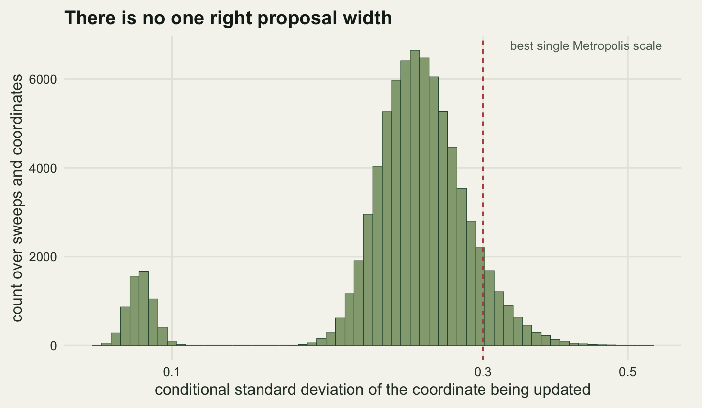
0.0768 0.5380 7.0028 The slice sweep needed no tuning of any kind: a width of one was written down once and used for all thirteen awkward conditionals, delivering 0.002883 effective draws per density evaluation on the worst-mixing quantity. The Metropolis-within-Gibbs version, with a single proposal scale searched over five values spanning a factor of 24, tops out at 0.001868 and bottoms out at 0.000284. The untuned slice version is 1.54 times the tuned Metropolis one and 10.2 times the worst, and they agree on the answer: a scheme-level log rate of 2.1925 against 2.2014, and a between-margin standard deviation of 0.4016 against 0.4014.
The reason a single Metropolis scale cannot win is in the last line of output. Over the run and across the thirteen coordinates the conditional standard deviation ranges from 0.0768 to 0.538, a factor of 7: the scheme-level rate has a tight conditional throughout, while the margin offsets widen and narrow as the between-margin standard deviation is resampled, its own posterior running from 0.2592 to 0.618. No single proposal scale is right for all of them, and no reason it should be. The slice update finds the local width every time, at 5.9 density evaluations per coordinate.
What one iteration costs
Acceptance rate is the wrong summary for a slice sampler, because it accepts by construction. The number playing the same role is the count of density evaluations per iteration, and it is never one. Putting the three samplers in this cluster on one currency needs a Hamiltonian version of the first target, which is short because the gradient of \(a\theta - b e^{\theta}\) is written down rather than differentiated.
pot <- function(th) -(a_post * th - b_post * exp(th))
grad_pot <- function(th) b_post * exp(th) - a_post

hmc_chain <- function(x0, eps, n_step, n_iter, seed) {
  set.seed(seed)
  out <- numeric(n_iter); q <- x0; uq <- pot(q); taken <- 0L
  for (it in seq_len(n_iter)) {
    p <- rnorm(1); qn <- q; pn <- p - 0.5 * eps * grad_pot(qn)
    for (i in seq_len(n_step)) {
      qn <- qn + eps * pn
      if (i < n_step) pn <- pn - eps * grad_pot(qn)
    }
    pn <- pn - 0.5 * eps * grad_pot(qn)
    un <- pot(qn); dh <- un + 0.5 * pn^2 - uq - 0.5 * p^2
    if (is.finite(dh) && log(runif(1)) < -dh) {
      q <- qn; uq <- un; taken <- taken + 1L
    }
    out[it] <- q
  }
  list(draws = out, evals = n_iter * (n_step + 1), accept = taken / n_iter)
}

hmc_steps <- 6
hmc_sweep <- data.frame(mult = mult_grid, eff = NA_real_, accept = NA_real_)
for (i in seq_along(mult_grid)) {
  hr <- hmc_chain(mean_exact, mult_grid[i] * sd_exact, hmc_steps,
                  floor(budget / (hmc_steps + 1)), 808)
  hmc_sweep$eff[i] <- ess_series(hr$draws) / hr$evals
  hmc_sweep$accept[i] <- hr$accept
}
hmc_ok <- !is.na(hmc_sweep$eff)
print(round(hmc_sweep, 6))
mult eff accept
1 0.031623 0.000613 0.999825
2 0.056234 0.002199 0.999825
3 0.100000 0.014566 0.999475
4 0.177828 0.050409 0.998775
5 0.316228 0.142857 0.993875
6 0.562341 0.142857 0.994225
7 1.000000 0.000160 0.999475
8 1.778279 0.004571 0.616031
9 3.162278 0.000186 0.000175
10 5.623413 NA 0.000000
11 10.000000 NA 0.000000
12 17.782794 NA 0.000000
13 31.622777 NA 0.000000
14 56.234133 NA 0.000000
15 100.000000 NA 0.000000
16 177.827941 NA 0.000000
17 316.227766 NA 0.000000cost <- data.frame(
sampler = c("slice", "random-walk Metropolis", "Hamiltonian"),
evals_per_iter = c(swp$per_iter[which.max(swp$slice)], 1, hmc_steps + 1),
best_eff = c(max(swp$slice), max(swp$metrop), max(hmc_sweep$eff, na.rm = TRUE)),
worst_eff = c(min(swp$slice), min(swp$metrop), min(hmc_sweep$eff, na.rm = TRUE)),
settings_alive = c(nrow(swp), nrow(swp), sum(hmc_ok)))
cost$tuning_span <- cost$best_eff / cost$worst_eff
print(cbind(cost[, c("sampler", "settings_alive")], round(cost[, 2:4], 5),
tuning_span = round(cost$tuning_span, 1))) sampler settings_alive evals_per_iter best_eff worst_eff
1 slice 17 4.91002 0.19868 0.00891
2 random-walk Metropolis 17 1.00000 0.21886 0.00030
3 Hamiltonian 9 7.00000 0.14286 0.00016
tuning_span
1 22.3
2 719.2
3 890.8print(round(c(hmc_dead_settings = sum(!hmc_ok),
hmc_first_dead_mult = min(mult_grid[!hmc_ok]),
slice_evals_low = min(swp$per_iter),
slice_evals_high = max(swp$per_iter)), 4)) hmc_dead_settings hmc_first_dead_mult slice_evals_low slice_evals_high
8.0000 5.6234 4.8603 107.6289 Three readings. First, the slice sampler costs 4.91 density evaluations per iteration at its best setting and between 4.86 and 107.63 across the sweep, so any comparison quoted per iteration flatters it by roughly that factor. Second, at their best settings the three are within a small factor of each other, 0.1987, 0.2189 and 0.1429 effective draws per evaluation: a smooth one-dimensional posterior offers a clever method very little to exploit. Third, the tuning spans differ by far more than the peaks do, 22.3 for the slice sampler against 719.2 for the random walk and 890.8 for the Hamiltonian sampler over the settings where it still moved. It stopped moving entirely at 8 of the 17 step sizes tried, every one above 5.62 posterior standard deviations, where the integrator diverges and nothing is ever accepted; its curve also has a hole in the middle of its working range, at the step size where the trajectory returns to where it started, which the trajectory-length sweep in the Hamiltonian post documents.
The honest limit
Coordinate-wise slice sampling inherits the weakness every coordinate-wise method has. The correlated-pair section measured it: a factor of 17 lost as the ridge sharpens, essentially the factor the coordinate-wise random walk loses, because no cleverness about how far to move along an axis compensates for moving along the wrong axis. Multivariate slice samplers do address this, from the hyperrectangle and reflective schemes in Neal (2003) to the elliptical version of Murray, Adams and MacKay (2010) for Gaussian priors, but they are far more work than the thirty lines above and none of them is in this post.
The step-out bound is a tuning parameter wearing a disguise. A finite cap keeps the sampler valid while making it behave like a random walk exactly where the random walk was already failing, measured above as a factor of 10.4 in the error on a tail quantile. Setting it high enough never to bind is the right default, and it leaves the sampler with no bound on how much work one iteration can do, which is uncomfortable in a production loop. Neal’s doubling procedure, which grows the interval geometrically and pays for it with an extra acceptance test, is the standard answer and is not implemented here.
The third limit is what these numbers extrapolate to. Every target here is small and every density evaluation is cheap, which is the regime where an iteration costing 4.9 evaluations instead of one is a detail. On a likelihood that takes a second, that factor is the whole story, and a tuned random walk getting 22 per cent of the effective draws per iteration for a fifth of the evaluations may be the right choice. The case for slice sampling was never speed. It is that the version you write down without thinking is usually within a small factor of the best one, which for the random walk is not true: over the same sweep its worst setting returned 0.139 per cent of its best. One caveat belongs with the numbers rather than the method: the effective sample size estimator stops at the chain length, so every figure for a sampler producing near-independent draws is a floor, and the slice sampler’s estimate came back as the exact chain length at several settings in the tuning sweep.
Where to go next
The natural next step is a Gibbs sweep over a model with more structure than twelve margins and one variance component. Nothing in the slice-within-Gibbs section needs modifying for several variance components or a non-conjugate prior on a dispersion parameter, because the update never needed to know anything about a conditional except how to evaluate it. The question this post did not ask is what happens when the width is adapted during warm-up rather than guessed, which is what production implementations do, and whether that buys anything measurable given how flat the curve above already is.
References
Neal RM 2003 Annals of Statistics 31(3):705-767 (10.1214/aos/1056562461)
Damlen P, Wakefield J, Walker S 1999 Journal of the Royal Statistical Society Series B 61(2):331-344 (10.1111/1467-9868.00179)
Higdon DM 1998 Journal of the American Statistical Association 93(442):585-595 (10.1080/01621459.1998.10473712)
Roberts GO, Rosenthal JS 1999 Journal of the Royal Statistical Society Series B 61(3):643-660 (10.1111/1467-9868.00198)
Mengersen KL, Tweedie RL 1996 Annals of Statistics 24(1):101-121 (10.1214/aos/1033066201)
Murray I, Adams RP, MacKay DJC 2010 Proceedings of Machine Learning Research 9:541-548
Vehtari A, Gelman A, Simpson D, Carpenter B, Burkner PC 2021 Bayesian Analysis 16(2):667-718 (10.1214/20-BA1221)
Gelman A, Carlin JB, Stern HS, Dunson DB, Vehtari A, Rubin DB 2013 Bayesian Data Analysis, 3rd edition (ISBN 978-1-4398-4095-5)