library(ggplot2)
library(patchwork)

te_paper  <- "#f5f4ee"
te_ink    <- "#16241d"
te_body   <- "#2c3a31"
te_forest <- "#275139"
te_rust   <- "#b5534e"
te_gold   <- "#c9b458"
te_line   <- "#dad9ca"

theme_datasheet <- function() {
  theme_minimal(base_size = 12) +
    theme(plot.background  = element_rect(fill = te_paper, colour = NA),
          panel.background = element_rect(fill = te_paper, colour = NA),
          panel.grid.major = element_line(colour = te_line, linewidth = 0.3),
          panel.grid.minor = element_blank(),
          text             = element_text(colour = te_body),
          plot.title       = element_text(colour = te_ink, face = "bold"),
          plot.subtitle    = element_text(colour = te_body),
          axis.text        = element_text(colour = te_body))
}Log-linear models for three-way count tables
R
GLM
contingency tables
log-linear models
simulation
ecology tutorial
A three-way table of nest counts fitted as nested Poisson GLMs in R: marginal versus conditional independence, and which term guarantees a safe collapse.
A shorebird warden has three seasons of nest records from one stretch of coast. Each nest sits in one of three habitats (dune, saltmarsh edge, shingle), each was either given a predator exclosure or left open, and each either fledged at least one chick or failed. The whole data set fits on an index card as a table of twelve counts. The obvious analysis sums over habitat, draws a two by two table of exclosure against outcome, and runs a chi-square test on it. The less obvious analysis keeps all three variables and asks which associations the twelve counts actually need.
The two analyses answer different questions, and they can disagree completely. The disagreement itself is already on this site: a Simpson reversal in checking a CNDD analysis, and the point that a conditional and a marginal odds ratio differ even without confounding in g-computation and standardisation. The post on behaviour sequences as Markov chains runs likelihood ratio tests on two and three way transition tables by hand, and it and the Hardy-Weinberg post have already measured how the chi-square approximation behaves in sparse cells, so that is not the subject here. This post is about the model family underneath all of them. In a log-linear model each of those statements (the association survives summing, the association is confounded, the two variables are independent within habitat) is a single term that the model keeps or drops, and the ordinary glm() with a Poisson family fits every one of them.
A count table is a Poisson GLM
Write X for the exclosure, Y for the outcome and Z for the habitat. A log-linear model treats the twelve cell counts as the response of a Poisson regression whose predictors are the three factors and their interactions. The models are named by their highest terms in brackets: [XY][XZ][YZ] contains every two factor interaction and no three factor one, which in glm() is x * y + x * z + y * z; [XZ][YZ] drops the exclosure by outcome term, which says that exclosure and outcome are independent within every habitat. The models are hierarchical, so a bracket implies all of its lower terms.
The generating side works directly on the log scale of the cell probabilities, so every scenario below is a choice of log-linear terms. Habitat effects are a strength times the scores minus one, zero and one for dune, saltmarsh edge and shingle, and the habitat main effect is set so that each habitat holds a third of the nests.
hab_lev  <- c("dune", "saltmarsh", "shingle")
n_hab    <- length(hab_lev)
hab_sc   <- c(-1, 0, 1)                  # habitat scores
n_nest   <- 400                          # nests in one table
alpha_lev <- 0.05
cells <- expand.grid(x = 0:1, y = 0:1, z = seq_len(n_hab))

# cell probabilities from log-linear terms
cell_prob <- function(xy = 0, xz = 0, yz = 0, x0 = -0.3, y0 = 0.2) {
  eta <- x0 * cells$x + y0 * cells$y + xy * cells$x * cells$y +
         xz * hab_sc[cells$z] * cells$x + yz * hab_sc[cells$z] * cells$y
  w <- exp(eta)
  w / ave(w, cells$z, FUN = sum) / n_hab          # equal nests per habitat
}
as_frame <- function(counts) {
  data.frame(x = factor(cells$x, labels = c("open", "exclosure")),
             y = factor(cells$y, labels = c("failed", "fledged")),
             z = factor(hab_lev[cells$z], levels = hab_lev), n = counts)
}
The first table comes from a truth in which exclosures do nothing. Wardens put more of them on shingle, where they are easiest to erect, and fledging success is also highest there; the strengths of both habitat effects are set to 1 on the log scale before anything is drawn.
str_xz <- 1; str_yz <- 1
set.seed(2508)
nests <- as_frame(as.vector(rmultinom(1, n_nest, cell_prob(xz = str_xz, yz = str_yz))))
ladder <- list(
  "[XYZ]"        = n ~ x * y * z,
  "[XY][XZ][YZ]" = n ~ x * y + x * z + y * z,
  "[XZ][YZ]"     = n ~ x * z + y * z,
  "[XY][YZ]"     = n ~ x * y + y * z,
  "[XY][XZ]"     = n ~ x * y + x * z,
  "[X][YZ]"      = n ~ x + y * z,
  "[Y][XZ]"      = n ~ y + x * z,
  "[Z][XY]"      = n ~ z + x * y,
  "[X][Y][Z]"    = n ~ x + y + z)
fits <- lapply(ladder, glm, family = poisson, data = nests)
lad <- data.frame(model = names(ladder),
                  G2 = vapply(fits, deviance, 0),
                  df = vapply(fits, df.residual, 0))
lad$crit <- qchisq(1 - alpha_lev, pmax(lad$df, 1))
lad$p <- ifelse(lad$df > 0, pchisq(lad$G2, lad$df, lower.tail = FALSE), NA)
# the same deviances by iterative proportional fitting
tab3 <- xtabs(n ~ x + y + z, data = nests)
ll_ci  <- loglin(tab3, list(c(1, 3), c(2, 3)), print = FALSE)
ll_nt  <- loglin(tab3, list(c(1, 2), c(1, 3), c(2, 3)), print = FALSE, eps = 1e-8, iter = 200)
ipf_gap <- max(abs(c(ll_ci$lrt - lad$G2[lad$model == "[XZ][YZ]"],
                     ll_nt$lrt - lad$G2[lad$model == "[XY][XZ][YZ]"])))
# the collapsed two by two table
tab2 <- xtabs(n ~ x + y, data = nests)
marg_test <- chisq.test(tab2, correct = FALSE)
marg_lor <- log(tab2[1, 1] * tab2[2, 2] / (tab2[1, 2] * tab2[2, 1]))
lad
model G2 df crit p
[XYZ] [XYZ] 7.993606e-15 0 3.841459 NA
[XY][XZ][YZ] [XY][XZ][YZ] 4.181301e-01 2 5.991465 8.113425e-01
[XZ][YZ] [XZ][YZ] 7.866761e-01 3 7.814728 8.526512e-01
[XY][YZ] [XY][YZ] 5.504860e+01 4 9.487729 3.173678e-11
[XY][XZ] [XY][XZ] 4.922441e+01 4 9.487729 5.242073e-10
[X][YZ] [X][YZ] 5.972928e+01 5 11.070498 1.382534e-11
[Y][XZ] [Y][XZ] 5.390509e+01 5 11.070498 2.192103e-10
[Z][XY] [Z][XY] 1.081670e+02 6 12.591587 4.931600e-21
[X][Y][Z] [X][Y][Z] 1.128477e+02 7 14.067140 2.354168e-21loglin() fits the same models by iterative proportional fitting, which is how log-linear models were fitted before generalised linear models existed, and its likelihood ratio statistics agree with the Poisson deviances to 1.0e-14. The deviance of a log-linear model is the G-squared statistic for that model against the saturated one, with degrees of freedom equal to the number of terms the model leaves out.
In this table the conditional independence model [XZ][YZ] has a deviance of 0.79 on 3 degrees of freedom (p = 0.853), which is the truth. The collapsed table tells another story. Summed over habitat, the exclosed nests have a log odds ratio of fledging of 0.44 against open nests, and the chi-square test on that two by two table gives 4.67 on one degree of freedom, p = 0.031.
lad_plot <- lad[lad$df > 0, ]
lad_plot$model <- factor(lad_plot$model, levels = rev(lad_plot$model))
lad_plot$verdict <- ifelse(lad_plot$G2 > lad_plot$crit, "rejected", "not rejected")
ggplot(lad_plot, aes(y = model)) +
  geom_point(aes(x = crit), shape = 124, size = 6, colour = te_body) +
  geom_point(aes(x = G2, colour = verdict), size = 3) +
  geom_text(aes(x = G2, label = sprintf("df %d", df)), nudge_y = 0.35,
            size = 3, colour = te_body) +
  scale_x_log10() +
  scale_colour_manual(values = c("not rejected" = te_forest, "rejected" = te_rust), name = NULL) +
  labs(x = "deviance (G-squared), log scale", y = NULL,
       title = "The ladder of models for one table",
       subtitle = "vertical ticks: five per cent critical value for each model's df") +
theme_datasheet() + theme(legend.position = "bottom")![Nine models listed down the left, from [XY][XZ][YZ] at the top to [X][Y][Z] at the bottom, with deviance on a logarithmic horizontal axis from below one to above one hundred. A short vertical tick on each row marks that model's five per cent critical value, between about six and fourteen. Two green points, [XY][XZ][YZ] with 2 df and [XZ][YZ] with 3 df, sit well to the left of their ticks, below one. The other seven points are rust and sit far to the right of their ticks: the four models with 4 or 5 df at about fifty to sixty, and [Z][XY] and [X][Y][Z] above one hundred.](index_files/figure-html/fig-ladder-1.png)
Every model that drops the habitat by outcome term or the habitat by exclosure term is thrown out, and the only simpler model the table accepts is the one without the exclosure by outcome term. Read the other way, the exclosure by outcome association in the collapsed table is carried entirely by the two habitat terms.
The Poisson fit and the logistic regression of outcome on exclosure and habitat are the same model written for two sampling schemes. Birch 1963 showed for three way tables that the maximum likelihood estimates are the same whether the counts are independent Poisson variables, one multinomial with a fixed total, or several multinomials with fixed margin totals, as long as the model contains the terms for the fixed margins. The check is numerical.
wide <- reshape(nests, idvar = c("x", "z"), timevar = "y", direction = "wide")
fit_logit <- glm(cbind(n.fledged, n.failed) ~ x + z, family = binomial, data = wide,
                 control = glm.control(epsilon = 1e-12, maxit = 50))
fit_nt <- glm(n ~ x * y + x * z + y * z, family = poisson, data = nests,
              control = glm.control(epsilon = 1e-12, maxit = 50))
pairs_cf <- c(xexclosure = "xexclosure:yfledged", zsaltmarsh = "yfledged:zsaltmarsh",
              zshingle = "yfledged:zshingle")
cf_gap <- max(abs(coef(fit_logit)[names(pairs_cf)] - coef(fit_nt)[pairs_cf]))
dev_gap <- abs(deviance(fit_logit) - deviance(fit_nt))
lor_nt <- unname(coef(fit_nt)["xexclosure:yfledged"])
The exclosure coefficient of the logistic regression and the exclosure by outcome term of [XY][XZ][YZ] are both -0.1418; across the three shared coefficients the largest difference is 2.1e-15, and the two residual deviances differ by 6.6e-15. A logistic regression with only main effects is the log-linear model with every two factor term and no three factor one. Adding an exclosure by habitat interaction to the logistic regression is adding the [XYZ] term.
Marginal and conditional independence are different models
One table proves nothing about rates. The measurement is how often the collapsed chi-square test rejects when exclosures truly do nothing within any habitat, as the two habitat terms grow. Next to it runs the test that matches the truth, the deviance of [XZ][YZ] on 3 degrees of freedom. For a two by two by K table that deviance is the sum over habitats of the two by two G-squared statistics, so it vectorises without a fitting loop, and its equality with the glm() deviance is checked on the first replicate.
g2_2x2 <- function(a, b, c2, d) {
  tot <- a + b + c2 + d
  term <- function(o, e) ifelse(o > 0, o * log(o / e), 0)
  2 * (term(a, (a + c2) * (a + b) / tot) + term(b, (b + d) * (a + b) / tot) +
       term(c2, (a + c2) * (c2 + d) / tot) + term(d, (b + d) * (c2 + d) / tot))
}
pearson_2x2 <- function(a, b, c2, d) {
  tot <- a + b + c2 + d
  tot * (a * d - b * c2)^2 / ((a + b) * (c2 + d) * (a + c2) * (b + d))
}
cell_id <- function(x, y, z) which(cells$x == x & cells$y == y & cells$z == z)
two_tests <- function(cnt) {
  mg <- function(x, y) colSums(cnt[vapply(seq_len(n_hab), function(z) cell_id(x, y, z), 0), , drop = FALSE])
  marg <- pearson_2x2(mg(0, 0), mg(1, 0), mg(0, 1), mg(1, 1))
  cond <- Reduce(`+`, lapply(seq_len(n_hab), function(z)
    g2_2x2(cnt[cell_id(0, 0, z), ], cnt[cell_id(1, 0, z), ],
           cnt[cell_id(0, 1, z), ], cnt[cell_id(1, 1, z), ])))
  cbind(marg = marg > qchisq(1 - alpha_lev, 1), cond = cond > qchisq(1 - alpha_lev, n_hab),
        cond_stat = cond, marg_stat = marg)
}
n_rep <- 10000                               # fixed before any rate was inspected
xz_grid <- c(0, 0.25, 0.5, 0.75, 1, 1.25, 1.5)
yz_grid <- c(0, 0.5, 1, 1.5)
grid_tab <- expand.grid(xz = xz_grid, yz = yz_grid)
set.seed(4417)
grid_res <- t(mapply(function(a, b) {
  cnt <- rmultinom(n_rep, n_nest, cell_prob(xz = a, yz = b))
  tt <- two_tests(cnt)
  c(marg = mean(tt[, "marg"]), cond = mean(tt[, "cond"]),
    first_cond = unname(tt[1, "cond_stat"]), first_marg = unname(tt[1, "marg_stat"]), cnt[, 1])
}, grid_tab$xz, grid_tab$yz))
grid_tab$marg <- grid_res[, "marg"]; grid_tab$cond <- grid_res[, "cond"]
first_fit <- glm(n ~ x * z + y * z, family = poisson,
                 data = as_frame(grid_res[nrow(grid_res), -(1:4)]))
first_gap <- abs(deviance(first_fit) - grid_res[nrow(grid_res), "first_cond"])
first_chisq <- unname(chisq.test(xtabs(n ~ x + y, data = as_frame(grid_res[nrow(grid_res), -(1:4)])),
                                 correct = FALSE)$statistic)
first_gap <- max(first_gap, abs(first_chisq - grid_res[nrow(grid_res), "first_marg"]))
mcse_max <- sqrt(0.25 / n_rep)
rate_at <- function(a, b, col) grid_tab[[col]][grid_tab$xz == a & grid_tab$yz == b]
marg_noyz <- grid_tab$marg[grid_tab$yz == 0]
marg_noxz <- grid_tab$marg[grid_tab$xz == 0]
cond_range <- range(grid_tab$cond)
cond_max_at <- unlist(grid_tab[which.max(grid_tab$cond), c("xz", "yz")])
thin_cell <- n_nest * min(cell_prob(xz = cond_max_at[1], yz = cond_max_at[2]))
The shortcut matches glm() and chisq.test() on the check replicate to 8.9e-15. With 10000 tables of 400 nests at each of the 28 grid points, the Monte Carlo standard error of any rate is at most 0.005.
grid_long <- rbind(
  data.frame(grid_tab[, c("xz", "yz")], rate = grid_tab$marg, test = "collapsed table, chi-square on 1 df"),
  data.frame(grid_tab[, c("xz", "yz")], rate = grid_tab$cond, test = "[XZ][YZ] deviance on 3 df"))
grid_long$test <- factor(grid_long$test, levels = unique(grid_long$test))
grid_long$yz_lab <- factor(sprintf("habitat on outcome %.1f", grid_long$yz),
                           levels = sprintf("habitat on outcome %.1f", yz_grid))
grid_long$mcse <- sqrt(grid_long$rate * (1 - grid_long$rate) / n_rep)
ggplot(grid_long, aes(xz, rate, colour = yz_lab, linetype = yz_lab)) +
  geom_hline(yintercept = alpha_lev, colour = te_body, linetype = "dashed", linewidth = 0.5) +
  geom_errorbar(aes(ymin = rate - 2 * mcse, ymax = rate + 2 * mcse), width = 0.04, linewidth = 0.4) +
  geom_line(linewidth = 0.9) + geom_point(size = 1.8) +
  facet_wrap(~ test) +
  scale_colour_manual(values = c(te_body, te_gold, te_forest, te_rust), name = NULL) +
  scale_linetype_manual(values = c("dotted", "solid", "solid", "solid"), name = NULL) +
  scale_y_continuous(limits = c(0, 1)) +
  guides(colour = guide_legend(nrow = 2), linetype = guide_legend(nrow = 2)) +
  labs(x = "strength of the habitat by exclosure term", y = "rejection rate",
       title = "No exclosure effect in any habitat",
       subtitle = "dashed line: five per cent; bars: two Monte Carlo standard errors") +
  theme_datasheet() +
  theme(legend.position = "bottom", strip.text = element_text(colour = te_ink))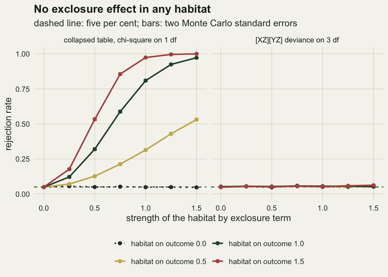
When either habitat term is zero the collapsed test holds its level: along the row with no habitat effect on outcome its rejection rate stays between 0.047 and 0.056, and along the column with no habitat effect on exclosure use between 0.048 and 0.049. Once both are present it climbs fast. At strength 0.5 for both terms it rejects 12.7 per cent of tables, at 1 for both 80.9 per cent, and at 1.5 for both 99.97 per cent. Swapping the two strengths hardly changes the rate: at 1.5 on exclosure use and 0.5 on outcome it is 53.1 per cent, and at 0.5 on exclosure use and 1.5 on outcome 53.3 per cent, a difference smaller than its own Monte Carlo standard error.
The deviance of [XZ][YZ] is a test of the right hypothesis, and across the whole grid its rejection rate runs from 0.047 to 0.062. That is a little above five per cent over much of the grid, with the highest rate at exclosure strength 1.50 and outcome strength 1.50, where the thinnest cell expects 4.1 nests. A small liberal excess of this size is the sparse-cell approximation discussed in the neighbouring posts (there in the conservative direction), and nothing like the collapsed test.
The collapsed chi-square is not a bad test. It is a test of the model [X][Y] for the two by two margin, which is a different hypothesis from [XZ][YZ] for the three way table, and on this grid it answers its own question correctly: summed over habitat, exclosed nests really do fledge at a different rate, because they sit disproportionately in the habitat where nests fledge. Which of the two hypotheses the warden cares about is a design question, not a statistical one.
Which term guarantees collapsing
The collapsed odds ratio is guaranteed to equal the within-habitat odds ratio when the table has no three factor term and at least one of the two habitat terms is zero in the log-linear model. Agresti 2013 states it for three way tables as: the XY marginal and conditional odds ratios are identical if Z and X are conditionally independent, or if Z and Y are conditionally independent, which are the models [XY][YZ] and [XY][XZ]. Both are conditional statements, given the third variable. That is where a randomised exclosure trial catches people out: coin-flip allocation makes exclosure and habitat independent in the margin, which is not the same thing.
Four truths, each with a within-habitat log odds ratio of 0.8 for exclosure on fledging. The first two satisfy the rule. The third is the randomised trial: half the nests in every habitat get an exclosure, and fledging follows a logistic model with an exclosure effect and a habitat effect and no interaction between them. The fourth has both habitat terms, as in the first table. The population values come from the exact cell probabilities; the replicate means come from tables of 400 nests.
lor_true <- 0.8; hab_str <- 1.2
exact_marg_lor <- function(p) {
  m <- tapply(p, list(cells$x, cells$y), sum)
  log(m[1, 1] * m[2, 2] / (m[1, 2] * m[2, 1]))
}
exact_cond_lor <- function(p, a = "x", b = "y") {
  vapply(split(seq_along(p), cells[[setdiff(c("x", "y", "z"), c(a, b))]]), function(i) {
    q <- p[i]; ca <- cells[[a]][i]; cb <- cells[[b]][i]
    if (b == "z") {  # x by (first vs last habitat), given y
      k1 <- q[cb == 1]; k3 <- q[cb == n_hab]
      return(log(k1[ca[cb == 1] == 0] * k3[ca[cb == n_hab] == 1] /
                 (k1[ca[cb == 1] == 1] * k3[ca[cb == n_hab] == 0])))
    }
    log(q[ca == 0 & cb == 0] * q[ca == 1 & cb == 1] / (q[ca == 0 & cb == 1] * q[ca == 1 & cb == 0]))
  }, 0)
}
rand_prob <- function() {
  p_fl <- plogis(-0.2 + lor_true * cells$x + hab_str * hab_sc[cells$z])
  0.5 / n_hab * ifelse(cells$y == 1, p_fl, 1 - p_fl)
}
scen_lev <- c("[XY][YZ]", "[XY][XZ]", "randomised exclosures", "[XY][XZ][YZ]")
scen <- list(cell_prob(xy = lor_true, yz = hab_str),
             cell_prob(xy = lor_true, xz = hab_str),
             rand_prob(),
             cell_prob(xy = lor_true, xz = hab_str, yz = hab_str))
names(scen) <- scen_lev
xz_marg_lor <- function(p) {             # exclosure by shingle versus dune, summed over outcome
  m <- tapply(p, list(cells$x, cells$z), sum)
  log(m[1, 1] * m[2, n_hab] / (m[2, 1] * m[1, n_hab]))
}
pop <- data.frame(scenario = factor(scen_lev, levels = scen_lev),
  cond = vapply(scen, function(p) mean(exact_cond_lor(p)), 0),
  cond_spread = vapply(scen, function(p) diff(range(exact_cond_lor(p))), 0),
  marg = vapply(scen, exact_marg_lor, 0),
  xz_marg = vapply(scen, xz_marg_lor, 0),
  xz_given_y = vapply(scen, function(p) mean(exact_cond_lor(p, "x", "z")), 0))

n_col <- 2000
set.seed(7730)
reps <- do.call(rbind, lapply(scen_lev, function(s) {
  cnt <- rmultinom(n_col, n_nest, scen[[s]])
  mg <- function(x, y) colSums(cnt[cells$x == x & cells$y == y, ])
  marg <- log(mg(0, 0) * mg(1, 1) / (mg(0, 1) * mg(1, 0)))
  xmat <- model.matrix(~ factor(x) + factor(z), data = cells[cells$y == 1, ])
  cond <- apply(cnt, 2, function(v)
    glm.fit(xmat, cbind(v[cells$y == 1], v[cells$y == 0]), family = binomial())$coefficients[2])
  data.frame(scenario = factor(s, levels = scen_lev), marg = marg, cond = cond)
}))
rep_sum <- do.call(rbind, lapply(split(reps, reps$scenario), function(r)
  data.frame(scenario = r$scenario[1], marg = mean(r$marg), cond = mean(r$cond),
             diff = mean(r$marg - r$cond), diff_se = sd(r$marg - r$cond) / sqrt(nrow(r)))))
# does the fitted no-three-factor model see the XZ term in the randomised trial?
set.seed(7731)
n_xz <- 1000
cnt_r <- rmultinom(n_xz, n_nest, scen[["randomised exclosures"]])
xz_p <- apply(cnt_r, 2, function(v) {
  dd <- as_frame(v)
  full <- glm(n ~ x * y + x * z + y * z, family = poisson, data = dd)
  drop_xz <- glm(n ~ x * y + y * z, family = poisson, data = dd)
  pchisq(deviance(drop_xz) - deviance(full), n_hab - 1, lower.tail = FALSE)
})
xz_detect <- mean(xz_p < alpha_lev); xz_detect_se <- sqrt(xz_detect * (1 - xz_detect) / n_xz)
gap_ratio <- min(abs(rep_sum$diff[3:4])) / max(abs(rep_sum$diff[1:2]))
pop; rep_sum
scenario cond cond_spread marg
[XY][YZ] [XY][YZ] 0.8 4.440892e-16 0.8000000
[XY][XZ] [XY][XZ] 0.8 4.440892e-16 0.8000000
randomised exclosures randomised exclosures 0.8 1.332268e-15 0.6485601
[XY][XZ][YZ] [XY][XZ][YZ] 0.8 4.440892e-16 1.5593064
xz_marg xz_given_y
[XY][YZ] 3.997887e-01 -3.697785e-32
[XY][XZ] 2.400000e+00 2.400000e+00
randomised exclosures -2.220446e-16 -4.226454e-01
[XY][XZ][YZ] 2.799789e+00 2.400000e+00 scenario marg cond diff
[XY][YZ] [XY][YZ] 0.7952786 0.7983695 -0.003090909
[XY][XZ] [XY][XZ] 0.7996395 0.8024313 -0.002791847
randomised exclosures randomised exclosures 0.6493619 0.8060980 -0.156736131
[XY][XZ][YZ] [XY][XZ][YZ] 1.5629184 0.8014047 0.761513775
diff_se
[XY][YZ] 0.002286772
[XY][XZ] 0.002431762
randomised exclosures 0.002421900
[XY][XZ][YZ] 0.002879120The exact values settle the population question. Under [XY][YZ] and under [XY][XZ] the collapsed log odds ratio is 0.800 and 0.800, the within-habitat value. With both habitat terms present it is 1.559, nearly double. Under randomisation it is 0.649, smaller than the within-habitat 0.8 even though there is no confounding of any kind.
The randomised row is where the rule’s conditional wording matters. In the margin summed over outcome, exclosure and habitat are exactly independent there: the log odds ratio of an exclosure on shingle against dune is 0.000. Given the outcome, it is -0.423. Among nests that fledged, exclosed nests are over-represented in the poorer habitat, because an exclosure is one of the two ways to fledge; conditioning on the outcome induces the association. The [XZ] term of the log-linear model is that conditional quantity, so it is not zero, and neither condition for collapsing holds. The [XY][YZ] row shows the reverse case: there, exclosure and habitat are associated in the margin (log odds ratio 0.400) and independent given the outcome (0.000), and the table collapses exactly. Marginal independence is neither necessary nor sufficient; the sufficient condition is about the conditional term.
Whether a table of this size would reveal the induced term is a separate matter. Fitting [XY][XZ][YZ] and [XY][YZ] to 1000 randomised tables of 400 nests and testing the difference in deviance, the [XZ] term is detected in 25.7 per cent of them (Monte Carlo standard error 1.4 points). A warden who checks the condition by testing the term will usually be told that collapsing is fine.
The replicates agree with the exact values. Over 2000 tables per row, the mean difference between collapsed and within-habitat estimates is -0.0031 and -0.0028 for the two collapsible truths (standard errors 0.0023 and 0.0024), both within 1.4 standard errors of zero; it is -0.157 for the randomised trial and +0.762 with both habitat terms, at least 51 times larger.
A shrunken collapsed odds ratio under randomisation is not a biased estimate of anything. It is the population-averaged effect of fitting exclosures to every nest, which is the quantity g-computation and standardisation sets out to estimate. The log-linear reading adds only where that gap lives: in a two factor term that randomisation does not remove.
reps_long <- rbind(data.frame(scenario = reps$scenario, est = reps$cond, kind = "within habitat"),
                   data.frame(scenario = reps$scenario, est = reps$marg, kind = "collapsed table"))
reps_long$kind <- factor(reps_long$kind, levels = c("within habitat", "collapsed table"))
pop_long <- rbind(data.frame(scenario = pop$scenario, est = pop$cond, kind = "within habitat"),
                  data.frame(scenario = pop$scenario, est = pop$marg, kind = "collapsed table"))
pop_long$kind <- factor(pop_long$kind, levels = levels(reps_long$kind))
ggplot(reps_long, aes(est, scenario, fill = kind)) +
  geom_vline(xintercept = lor_true, colour = te_body, linetype = "dashed", linewidth = 0.5) +
  geom_boxplot(width = 0.55, outlier.size = 0.4, outlier.alpha = 0.4, colour = te_body,
               linewidth = 0.35, position = position_dodge(width = 0.7)) +
  geom_point(data = pop_long, aes(est, scenario, group = kind), shape = 23, size = 2.6,
             fill = te_paper, colour = te_ink, position = position_dodge(width = 0.7)) +
  scale_fill_manual(values = c(te_forest, te_gold), name = NULL) +
  scale_y_discrete(limits = rev(scen_lev)) +
  labs(x = "log odds ratio of fledging, exclosure against open", y = NULL,
       title = "Collapsing is safe in the first two rows only",
       subtitle = "boxes: 2000 tables each; diamonds: exact; dashed: truth") +
theme_datasheet() + theme(legend.position = "bottom")![Four rows of paired horizontal box plots of the log odds ratio of fledging, with a dashed vertical line at the true value of zero point eight and white diamonds for exact values. In the rows labelled [XY][YZ] and [XY][XZ] the gold collapsed box and the green within-habitat box are centred on the dashed line. In the randomised exclosures row the green box is centred on the line but the gold box sits to its left, centred near zero point six five. In the [XY][XZ][YZ] row the green box is on the line and the gold box sits far to the right, centred near one point five six.](index_files/figure-html/fig-collapse-1.png)
With three habitats the rule is not necessary
Whittemore 1978 showed that a table can be summed over a factor without changing the log-linear terms of the others under less restrictive conditions than the ones usually quoted. With three habitats this is easy to see. Keep the habitat by exclosure term at scores minus one, zero, one, keep the exclosure effect at 0.8, and let the habitat by outcome term take a free value on shingle while dune stays at minus one and saltmarsh at zero. The collapsed odds ratio is a smooth function of that shingle value, and it crosses the within-habitat value somewhere.
cex_prob <- function(yz_shingle, xz_str = 1, yz_vec = c(-1, 0, NA)) {
  yz_vec[n_hab] <- yz_shingle
  eta <- -0.3 * cells$x + 0.2 * cells$y + lor_true * cells$x * cells$y +
         xz_str * hab_sc[cells$z] * cells$x + yz_vec[cells$z] * cells$y
  w <- exp(eta)
  w / ave(w, cells$z, FUN = sum) / n_hab
}
shingle_seq <- seq(-3, 3, by = 0.05)
cex_curve <- data.frame(yz_shingle = shingle_seq,
                        marg = vapply(shingle_seq, function(s) exact_marg_lor(cex_prob(s)), 0))
root <- uniroot(function(s) exact_marg_lor(cex_prob(s)) - lor_true, c(-3, 0), tol = 1e-12)$root
p_root <- cex_prob(root)
root_cond <- exact_cond_lor(p_root)
# the two habitat terms at the root, as conditional log odds ratios (shingle vs dune)
root_xz <- mean(exact_cond_lor(p_root, "x", "z"))
root_yz <- log(p_root[cell_id(0, 0, 1)] * p_root[cell_id(0, 1, 3)] /
               (p_root[cell_id(0, 1, 1)] * p_root[cell_id(0, 0, 3)]))
# drop one habitat at a time and collapse the other two
drop_one <- vapply(seq_len(n_hab), function(h) {
  keep <- cells$z != h; m <- tapply(p_root[keep], list(cells$x[keep], cells$y[keep]), sum)
  log(m[1, 1] * m[2, 2] / (m[1, 2] * m[2, 1]))
}, 0)
# two habitats: closed-form shift of the collapsed log odds ratio, checked against exact tables
cells2 <- expand.grid(x = 0:1, y = 0:1, z = 0:1)
shift_formula <- function(g, d, e) {
  G <- exp(g); D <- exp(d); E <- exp(e)
  log(1 + G * (1 - D) * (1 - E) / ((1 + G * D) * (1 + G * E)))
}
shift_exact <- function(g, d, e, a = -0.3, b = 0.2) {
  eta <- a * cells2$x + b * cells2$y + lor_true * cells2$x * cells2$y + g * cells2$z +
         d * cells2$x * cells2$z + e * cells2$y * cells2$z
  m <- tapply(exp(eta), list(cells2$x, cells2$y), sum)
  log(m[1, 1] * m[2, 2] / (m[1, 2] * m[2, 1])) - lor_true
}
bin_grid <- expand.grid(g = seq(-6, 6, by = 1), d = seq(-2, 2, by = 0.25), e = seq(-2, 2, by = 0.25))
bin_grid$exact <- mapply(shift_exact, bin_grid$g, bin_grid$d, bin_grid$e)
bin_grid$formula <- with(bin_grid, shift_formula(g, d, e))
formula_err <- max(abs(bin_grid$exact - bin_grid$formula))
both_on <- bin_grid$d != 0 & bin_grid$e != 0
sign_match <- mean(sign(bin_grid$exact[both_on]) == sign(bin_grid$d[both_on] * bin_grid$e[both_on]))
zero_when_off <- max(abs(bin_grid$exact[!both_on]))
shift_even <- shift_exact(0, 1, 1); shift_uneven <- shift_exact(5, 1, 1)
The curve crosses the within-habitat value at a shingle value of -1.003. At that point the table has no three factor term (the within-habitat log odds ratios are 0.800, 0.800, 0.800), the habitat by exclosure term is far from zero (a log odds ratio of 2.00 for an exclosure on shingle against dune, given the outcome), and so is the habitat by outcome term, because saltmarsh sits one unit above the other two habitats. Yet the collapsed log odds ratio is exactly 0.8. The crossing is close to the symmetric point where dune and shingle share an outcome term: saltmarsh then carries the extra fledging success, and its exclosure use sits halfway between the other two habitats, so its excess falls almost equally on the exclosed and the open nests, and the confounding from dune and shingle cancels.
That kind of collapsibility is an accident of the particular set of habitats. Leave one habitat out and collapse the other two: without dune the collapsed log odds ratio is 0.559, without saltmarsh 0.798, without shingle 1.040. Only the dune and shingle pair comes close, because those two habitats have almost the same outcome term (minus one against the crossing value), so within that pair the conditional independence rule nearly holds. When the rule holds it holds in every subset of habitats, because a term that is zero stays zero when levels are dropped; the crossing on the left is a property of this one set of three.
With only two habitats there is no such accident, and the rule is necessary as well. Write the habitat main effect as g, the habitat by exclosure term as d and the habitat by outcome term as e, with G, D and E their exponentials. Summing over a binary habitat shifts the log odds ratio by log(1 + G(1 - D)(1 - E) / ((1 + GD)(1 + GE))), which follows from adding the two habitat layers cell by cell. The shift is zero only if d = 0 or e = 0, and its sign is the sign of d times e. The chunk checks the identity against exact tables over a grid of 3757 parameter combinations: the largest difference between formula and exact value is 1.58e-15, the sign matches in 100.0 per cent of the combinations with both terms present, and the largest shift with either term absent is 1.33e-15. The size of the shift depends on how the nests are split between habitats: with both terms at 1 it is 0.194 when g is 0 and only 0.0027 when g is 5, so a table dominated by one habitat can be nearly collapsible without either term being small.
drop_tab <- data.frame(dropped = factor(sprintf("without %s", hab_lev), levels = sprintf("without %s", hab_lev)),
                       lor = drop_one)
p_curve <- ggplot(cex_curve, aes(yz_shingle, marg)) +
  geom_hline(yintercept = lor_true, colour = te_body, linetype = "dashed", linewidth = 0.5) +
  geom_line(colour = te_forest, linewidth = 1) +
  geom_point(data = data.frame(yz_shingle = root, marg = lor_true), colour = te_rust, size = 3) +
  labs(x = "habitat by outcome term on shingle", y = "collapsed log odds ratio",
       title = "Three habitats", subtitle = "dashed: within-habitat value") +
  theme_datasheet()
p_drop <- ggplot(drop_tab, aes(lor, dropped)) +
  geom_vline(xintercept = lor_true, colour = te_body, linetype = "dashed", linewidth = 0.5) +
  geom_segment(aes(x = lor_true, xend = lor, yend = dropped), colour = te_line, linewidth = 1.2) +
  geom_point(colour = te_rust, size = 3) +
  labs(x = "collapsed log odds ratio", y = NULL,
       title = "Drop one habitat",
       subtitle = "dashed: within-habitat value") +
  theme_datasheet()
p_curve + p_drop + plot_annotation(theme = theme_datasheet())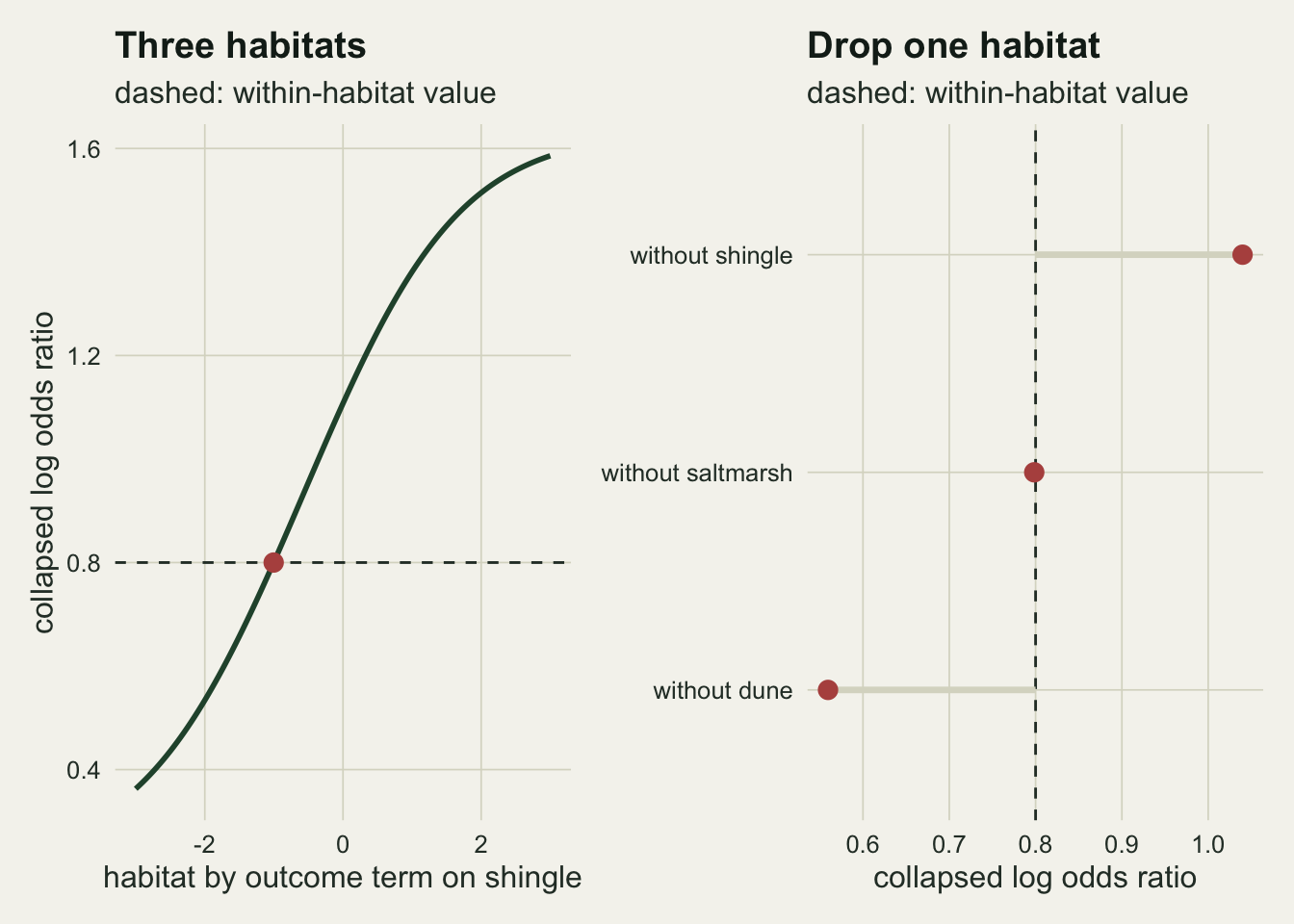
What to report
Name the model, not only the test. “Exclosure and fledging are independent within habitat, [XZ][YZ], deviance 0.79 on 3 degrees of freedom” says what was assumed and what was compared; “chi-square p = 0.031” on a collapsed table does not say which margin was summed over, and the reader cannot tell that the collapsed and three way analyses reach opposite verdicts on the same twelve counts.
Give the table. Twelve counts fit in one line of a results section, and every model in the ladder can be refitted from them in a few seconds. That is rarely true of anything else a paper reports.
If the analysis reports a collapsed association, state which two factor term justifies summing and how it was checked, and say whether the check was a term test on a table the size of this one. A non-significant [XZ] or [YZ] term is weak evidence at a few hundred nests.
If the design was randomised, say which odds ratio is reported. The within-habitat and the collapsed values are both legitimate and differ by construction; call one conditional and the other marginal and do not compare either with an odds ratio from another study that made the other choice.
When the outcome is a response and the other two are explanatory, fit the logistic regression and report it; it is the same model as the log-linear one with every explanatory interaction included, and its coefficients are the ones readers expect. The log-linear form earns its place when no variable is the response, or when the question is about which associations exist at all.
Honest limits
Every table here is two by two by three with a few hundred nests, fixed in total, from a single multinomial draw. Real nest records are clustered by site, season and observer, and a count of nests treated as independent multinomial trials inherits all the problems of pseudoreplication; the deviances above are valid only if each nest is an independent trial.
Habitat has three ordered levels with linear scores, and each habitat holds a third of the nests. The rejection rates in the grid depend on those choices and on the baseline rates, and they are not transferable to another design without rerunning the chunk. Both baseline rates sit near one half, which is why the two habitat strengths are nearly interchangeable in the grid; with a rare outcome they would not be.
The collapsibility statements are about log-linear terms, which for binary X and Y are log odds ratios. Risk differences and risk ratios obey different collapsibility conditions, and nothing here says anything about them.
The counterexample was built by solving for one parameter. It shows that the conditional independence condition is not necessary for collapsing a two by two by three table; it says nothing about how often such cancellation happens in real data, where it would require an unlikely balance between habitat terms.
The worked table is one draw. Its verdicts (collapsed test rejects, conditional model accepted) happen to agree with the grid, but at strength 1 for both habitat terms the collapsed test rejects in 81 per cent of tables, so 19 per cent of draws would have left the collapsed test silent, and the grid is the result.
References
Birch MW 1963 Journal of the Royal Statistical Society B 25(1):220-233 (10.1111/j.2517-6161.1963.tb00504.x)
Whittemore AS 1978 Journal of the Royal Statistical Society B 40(3):328-340 (10.1111/j.2517-6161.1978.tb01046.x)
Agresti A 2013 Categorical Data Analysis, 3rd edition (ISBN 978-0-470-46363-5)