library(ggplot2)

te_pal <- list(forest = "#275139", green = "#2f8f63", sage = "#93a87f",
               clay = "#b5534e", gold = "#cda23f", line = "#dad9ca",
               ink = "#16241d", paper = "#f5f4ee")

theme_te <- function() {
  theme_minimal(base_size = 12) +
    theme(panel.grid.minor = element_blank(),
          panel.grid.major = element_line(colour = "#e7e6dc"),
          plot.background = element_rect(fill = "#f5f4ee", colour = NA),
          panel.background = element_rect(fill = "#f5f4ee", colour = NA),
          plot.title = element_text(face = "bold", colour = te_pal$ink),
          axis.title = element_text(colour = "#2c3a31"),
          legend.position = "bottom")
}

## a 2x2 covariance matrix from two variances and a correlation
make_cov <- function(v1, v2, r) {
  matrix(c(v1, r * sqrt(v1 * v2), r * sqrt(v1 * v2), v2), 2, 2)
}

## the correlation implied by a 2x2 covariance matrix
cor_of <- function(S) S[1, 2] / sqrt(S[1, 1] * S[2, 2])

## simulate two traits measured k_rep times on each of n_ind individuals
sim_pair <- function(n_ind, k_rep, S_among, S_within) {
  A  <- matrix(rnorm(n_ind * 2), n_ind, 2) %*% chol(S_among)
  E  <- matrix(rnorm(n_ind * k_rep * 2), n_ind * k_rep, 2) %*% chol(S_within)
  id <- rep(seq_len(n_ind), each = k_rep)
  list(y = A[id, ] + E, id = id, n_ind = n_ind, k_rep = k_rep)
}

## the balanced-design moment estimator of the two covariance matrices
partition <- function(dat) {
  n_ind <- dat$n_ind
  k_rep <- dat$k_rep
  ybar  <- rowsum(dat$y, dat$id) / k_rep
  wth   <- dat$y - ybar[dat$id, ]
  S_w   <- crossprod(wth) / (n_ind * (k_rep - 1))
  S_b   <- crossprod(sweep(ybar, 2, colMeans(ybar))) * k_rep / (n_ind - 1)
  list(among = (S_b - S_w) / k_rep, within = S_w, means = ybar)
}Behavioural syndromes in R
R
behaviour
mixed models
repeatability
ecology tutorial
Fit a bivariate mixed model by hand in base R to separate a behavioural syndrome from the within-individual correlation in repeated ecological field data.
The field notebook says the same thing every year. Sixty great tits caught in the same winter wood, each one scored twice in a novel-environment box and twice on a feeder for latency to approach. The person doing the analysis pools all the scores, plots latency against exploration, draws a line through the cloud, and writes that bolder birds are more exploratory. The correlation is positive, the p-value is small, and the sentence goes into the paper as evidence of a behavioural syndrome.
The trouble is that the picture contains two entirely different sources of covariation and the pooled correlation mixes them. Some of the covariation is between birds: one bird really is bolder on average than another, and if that same bird is also more exploratory on average, that is the syndrome. Some of it is within birds: on the morning that a bird happened to approach the feeder quickly, it may also have moved around the novel box quickly, because it was hungry that morning, or warm, or because the observer was standing in a different place. That within-individual covariation is real, it is often large, and it has nothing to do with whether individuals differ consistently.
A behavioural syndrome, as the term is normally defined, is a correlation among individual means. It lives in the among-individual covariance matrix. The pooled scatter plot estimates something else: the phenotypic correlation, which is a weighted blend of the among-individual and within-individual correlations. The two numbers are different. Under conditions that occur routinely in behavioural data they have opposite signs, so the pooled plot can be a picture of a syndrome that does not exist, or a picture of the absence of a syndrome that does.
This post writes the decomposition down, checks it numerically, builds a case where the sign flips, fits the bivariate mixed model from scratch with optim and a Cholesky parameterisation, and then measures how precisely the among-individual correlation can actually be estimated. The last section produced the result I did not expect, and it changes the standard design advice.
A note on words, because the literature uses several. A behavioural type is one individual’s average position on one behavioural axis. Personality, or consistent individual difference, is the statement that those averages differ more than measurement noise alone would produce, which is what a repeatability quantifies. A behavioural syndrome is the statement that two of those averages covary. All three live in the among-individual part of the model, and all three are invisible to an analysis that treats every observation as an independent animal.
The one-trait version of this variance partition is in Adjusted repeatability in R; this post is the two-trait extension of exactly that model, so if the notion of splitting a variance into an among-individual and a within-individual piece is new, read that one first.
Four helpers do all the work. make_cov builds a 2 by 2 covariance matrix from two variances and a correlation, cor_of reads a correlation back out of one, sim_pair draws two traits measured repeatedly on the same individuals, and partition is the classical balanced-design moment estimator: within-individual scatter gives the residual matrix directly, among-individual scatter of the individual means gives the residual matrix plus k_rep times the among-individual matrix, and subtracting recovers the among-individual matrix. Everything below is base R and ggplot2.
Nothing here needs a package. The model has a closed-form covariance structure for balanced data, the likelihood is a multivariate normal, and optim is in base R. Writing it out is worth the twenty lines because the structure of the estimator is the thing being taught: once the two covariance matrices are visible as separate objects, the difference between the two correlations stops being an abstract warning and becomes a subtraction you can watch happen.
Two correlations, one data set
Write the model for two traits, indexed by \(t\), measured on individual \(i\) at occasion \(j\):
\[y_{tij} = \mu_t + a_{ti} + e_{tij}\]
The individual deviations \((a_{1i}, a_{2i})\) are drawn from a bivariate normal with covariance matrix \(\Sigma_{\text{ind}}\), and the residuals \((e_{1ij}, e_{2ij})\) from a bivariate normal with covariance matrix \(\Sigma_{\text{e}}\). The two are independent. Because they are independent, the covariance of the observed values adds:
\[\Sigma_{\text{P}} = \Sigma_{\text{ind}} + \Sigma_{\text{e}}\]
Divide through by the phenotypic standard deviations and the additive statement about covariances becomes a mixture statement about correlations. Write \(R_1\) and \(R_2\) for the repeatabilities of the two traits, \(r_{\text{ind}}\) for the among-individual correlation (the syndrome) and \(r_{\text{e}}\) for the within-individual correlation. Then
\[r_{\text{P}} = r_{\text{ind}} \sqrt{R_1 R_2} + r_{\text{e}} \sqrt{(1 - R_1)(1 - R_2)}\]
The weights are the geometric mean of the repeatabilities and the geometric mean of one minus the repeatabilities. They do not sum to one unless \(R_1 = R_2\), which is worth holding on to: this is a weighted blend but it is not an average in the everyday sense, and the phenotypic correlation is not bounded between the two component correlations only because the weights can both be small.
The within-individual correlation deserves better than the label of nuisance. It is a real biological quantity: it says how two behaviours move together within an animal across occasions, which is a statement about time budgets, state dependence and plasticity. A strongly negative within-individual correlation between foraging and resting is not measurement error; it is the fact that an afternoon has a fixed number of hours. Treating it as noise to be averaged away is the mistake that produces the pooled correlation in the first place.
rep1     <- 0.45
rep2     <- 0.25
r_among  <- 0.60
r_within <- -0.35

S_among  <- make_cov(1, 1, r_among)
S_within <- make_cov((1 - rep1) / rep1, (1 - rep2) / rep2, r_within)
S_pheno  <- S_among + S_within

r_pheno_direct   <- cor_of(S_pheno)
r_pheno_identity <- r_among * sqrt(rep1 * rep2) +
                    r_within * sqrt((1 - rep1) * (1 - rep2))

print(round(c(rep1 = rep1, rep2 = rep2,
              r_among = r_among, r_within = r_within,
              r_pheno_direct = r_pheno_direct,
              r_pheno_identity = r_pheno_identity,
              gap = r_pheno_direct - r_pheno_identity), 10))
rep1 rep2 r_among r_within
0.45000000 0.25000000 0.60000000 -0.35000000
r_pheno_direct r_pheno_identity gap
-0.02354545 -0.02354545 0.00000000 print(round(c(among_weight = sqrt(rep1 * rep2),
within_weight = sqrt((1 - rep1) * (1 - rep2)),
r_pheno_4dp = r_pheno_direct), 4)) among_weight within_weight r_pheno_4dp
0.3354 0.6423 -0.0235 The two routes agree. The direct route builds \(\Sigma_{\text{P}}\) by adding the matrices and reads the correlation off it; the identity route never forms \(\Sigma_{\text{P}}\) at all and works only with the four scalars. Both give -0.0235 and the printed gap is 0 at ten decimal places, which is what an algebraic identity should do.
Look at the numbers that produced it. The among-individual correlation is 0.6, a strong positive syndrome. The within-individual correlation is -0.35. The repeatabilities are 0.45 and 0.25, which are ordinary values for behavioural traits. The phenotypic correlation that comes out is -0.0235, which rounds to zero for any practical purpose. A researcher who pooled these observations would report no relationship between the two behaviours and would be wrong about the biology in the most complete way possible: there is a strong syndrome, and the pooled analysis cannot see it.
The weights are worth computing by hand here. With repeatabilities of 0.45 and 0.25, the among-individual weight is the square root of their product and the within-individual weight is the square root of the product of their complements. The second is much the larger of the two, which is why a within-individual correlation of -0.35 can cancel an among-individual correlation of 0.6 despite being smaller in magnitude. Low repeatability does not just shrink the syndrome; it hands most of the weight to the other correlation.
That is the algebra. The next chunk checks that data simulated from the model behave the same way, which is a different claim: the identity is exact for population parameters, and a finite sample only has to obey it approximately.
One thing the simulation cannot check, because it is built into the generating model, is the assumption of independence between the individual deviations and the residuals. Real behavioural data can violate it: an individual whose average is extreme may also be more variable across occasions, which is individual variation in plasticity rather than in mean. The model fitted here has no term for that, and neither does the pooled correlation, so the comparison between them is fair even though both are incomplete.
set.seed(20260727)

n_check <- 4000
k_check <- 8
dat_chk <- sim_pair(n_check, k_check, S_among, S_within)
prt_chk <- partition(dat_chk)

rep1_hat <- prt_chk$among[1, 1] / (prt_chk$among[1, 1] + prt_chk$within[1, 1])
rep2_hat <- prt_chk$among[2, 2] / (prt_chk$among[2, 2] + prt_chk$within[2, 2])

r_pheno_obs <- cor(dat_chk$y[, 1], dat_chk$y[, 2])
r_pheno_fit <- cor_of(prt_chk$among) * sqrt(rep1_hat * rep2_hat) +
               cor_of(prt_chk$within) * sqrt((1 - rep1_hat) * (1 - rep2_hat))

print(round(c(n_ind = n_check, k_rep = k_check, n_obs = n_check * k_check,
              rep1_hat = rep1_hat, rep2_hat = rep2_hat,
              r_among_hat = cor_of(prt_chk$among),
              r_within_hat = cor_of(prt_chk$within),
              r_pheno_observed = r_pheno_obs), 4))
n_ind k_rep n_obs rep1_hat
4000.0000 8.0000 32000.0000 0.4470
rep2_hat r_among_hat r_within_hat r_pheno_observed
0.2450 0.5779 -0.3497 -0.0347 print(round(c(r_pheno_observed = r_pheno_obs,
r_pheno_from_identity = r_pheno_fit,
gap = r_pheno_obs - r_pheno_fit), 6)) r_pheno_observed r_pheno_from_identity gap
-0.034731 -0.034687 -0.000044 With 4000 individuals measured 8 times each, the moment estimator returns repeatabilities of 0.447 and 0.245 against simulated values of 0.45 and 0.25, an among-individual correlation of 0.5779 against 0.6, and a within-individual correlation of -0.3497 against -0.35. Plugging those four estimates into the identity gives -0.034687, and the ordinary pooled correlation of all 32000 observations is -0.034731. The gap is -0.000044, which comes from the different degrees-of-freedom divisors in the two estimators rather than from any failure of the identity.
The estimated syndrome is 0.5779, the pooled correlation is -0.0347, and this is a sample of 32000 observations. Sample size does not help. The pooled correlation converges perfectly well; it just converges to the wrong quantity.
That last sentence is the whole argument in one line, and it is why this is not a power problem. A biased estimator with a huge sample gives a precise answer to a question nobody asked. Adding observations narrows the interval around the pooled correlation and does nothing at all to move it towards the syndrome.
Attenuation: the phenotypic correlation is a shrunken copy
Set the within-individual correlation to zero and the identity collapses to a single product:
\[r_{\text{P}} = r_{\text{ind}} \sqrt{R_1 R_2}\]
This is the same attenuation factor that appears whenever a correlation is computed between two variables measured with error, and it is the case people have in mind when they say that pooling “dilutes” the signal. It is worth separating from the general case, because it is the only situation in which the pooled correlation is guaranteed to be a conservative version of the syndrome: same sign, smaller magnitude, never larger.
The formula also runs backwards, and running it backwards is tempting and dangerous. Dividing an observed pooled correlation by the square root of the product of two estimated repeatabilities gives a disattenuated correlation, which is an old idea from psychometrics. It is unbiased only if the within-individual correlation really is zero, and the correction divides by a small and itself noisy number, so it inflates the sampling error along with the estimate. The bivariate model does the same job without either assumption.
The grid below covers six values of \(R_1\), three of \(R_2\) and three of \(r_{\text{ind}}\), and simulates a large data set at each combination.
set.seed(20260728)

rep_lv1 <- c(0.10, 0.20, 0.37, 0.55, 0.75, 0.95)
rep_lv2 <- c(0.15, 0.40, 0.80)
r_lv    <- c(0.25, 0.55, 0.85)
n_grid  <- 4000
k_grid  <- 6

att <- expand.grid(rep1 = rep_lv1, rep2 = rep_lv2, r_among = r_lv)
att$predicted <- att$r_among * sqrt(att$rep1 * att$rep2)
att$measured  <- NA_real_

for (i in seq_len(nrow(att))) {
  sa <- make_cov(1, 1, att$r_among[i])
  sw <- make_cov((1 - att$rep1[i]) / att$rep1[i],
                 (1 - att$rep2[i]) / att$rep2[i], 0)
  dd <- sim_pair(n_grid, k_grid, sa, sw)
  att$measured[i] <- cor(dd$y[, 1], dd$y[, 2])
}

att$gmr   <- sqrt(att$rep1 * att$rep2)
att$ratio <- att$measured / att$r_among

edge_lo <- sort(att$measured[att$rep1 == min(rep_lv1) & att$rep2 == min(rep_lv2)])
edge_hi <- sort(att$measured[att$rep1 == max(rep_lv1) & att$rep2 == max(rep_lv2)])
squash  <- diff(range(edge_hi)) / diff(range(edge_lo))

print(round(c(rep1_levels = rep_lv1), 4))
rep1_levels1 rep1_levels2 rep1_levels3 rep1_levels4 rep1_levels5 rep1_levels6
0.10 0.20 0.37 0.55 0.75 0.95 print(round(c(rep2_levels = rep_lv2), 4))rep2_levels1 rep2_levels2 rep2_levels3
0.15 0.40 0.80 print(round(c(r_among_levels = r_lv), 4))r_among_levels1 r_among_levels2 r_among_levels3
0.25 0.55 0.85 print(round(c(cells = nrow(att), n_ind = n_grid, k_rep = k_grid,
min_gmr = min(att$gmr), max_gmr = max(att$gmr),
max_gap = max(abs(att$measured - att$predicted)),
mean_abs_gap = mean(abs(att$measured - att$predicted)),
min_ratio = min(att$ratio),
max_ratio = max(att$ratio)), 4)) cells n_ind k_rep min_gmr max_gmr max_gap
54.0000 4000.0000 6.0000 0.1225 0.8718 0.0178
mean_abs_gap min_ratio max_ratio
0.0068 0.1057 0.9058 print(round(c(gmr_low = min(att$gmr), gmr_high = max(att$gmr),
low_edge = edge_lo, spread_low = diff(range(edge_lo)),
spread_high = diff(range(edge_hi)), squash_factor = squash), 4)) gmr_low gmr_high low_edge1 low_edge2 low_edge3
0.1225 0.8718 0.0344 0.0671 0.0899
spread_low spread_high squash_factor
0.0555 0.5202 9.3698 Across all 54 cells, each simulated with 4000 individuals and 6 repeats, the largest discrepancy between the measured pooled correlation and the predicted \(r_{\text{ind}}\sqrt{R_1 R_2}\) is 0.0178 and the mean absolute discrepancy is 0.0068. Those are Monte Carlo residuals at this sample size, not model error.
The grid deliberately includes a repeatability of 0.95, which is higher than almost any behavioural trait achieves, and one of 0.1, which is lower than most published estimates but not absurd for a single-trial assay. Between those extremes sits the range that matters in practice, and the important feature of the range is that the attenuation factor is a product: it takes two good repeatabilities to keep the pooled correlation honest, and one bad one is enough to ruin it.
The two ratio numbers are the ones to take away. The pooled correlation retains between 0.1057 and 0.9058 of the syndrome across this grid. At the bottom end, a syndrome of 0.85 between two traits with repeatabilities of 0.1 and 0.15 shows up in the pooled data at roughly a tenth of its size. It is not that the effect is small; it is that the measurement is diluted by a factor the analyst never computed.
ggplot(att, aes(gmr, measured, colour = factor(r_among))) +
  geom_abline(intercept = 0, slope = r_lv,
              colour = te_pal$sage, linewidth = 0.5, linetype = "22") +
  geom_point(size = 2.1, alpha = 0.9) +
  scale_colour_manual(values = c(te_pal$gold, te_pal$green, te_pal$forest),
                      name = "among-individual correlation") +
  labs(x = "geometric mean of the two repeatabilities",
       y = "measured phenotypic correlation") +
  theme_te()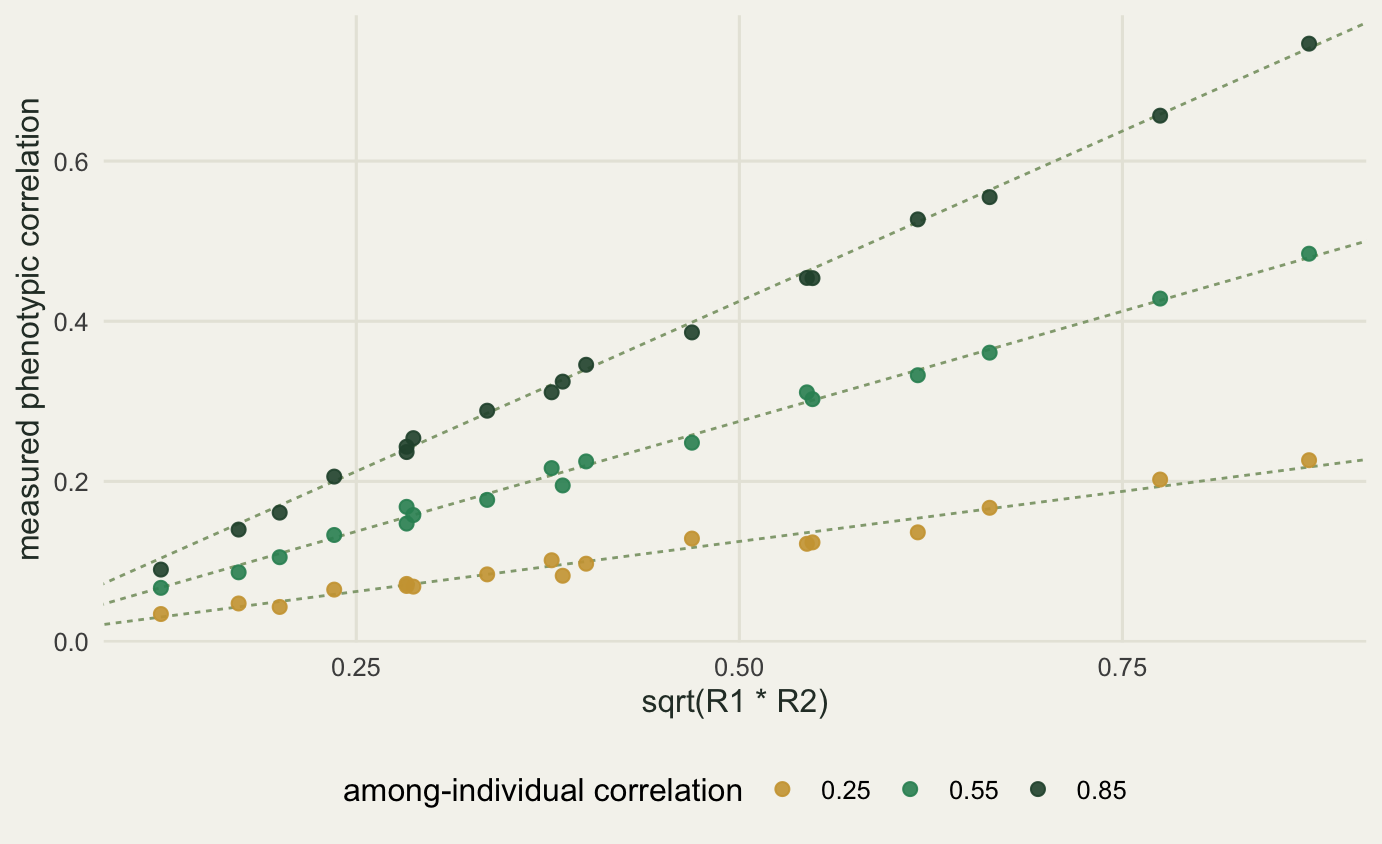
The figure makes the practical consequence visible. Read across the left-hand edge, where the geometric mean repeatability is 0.1225. The three fans have not merged: the points sit at 0.0344, 0.0671 and 0.0899, one clearly above the other. What has happened is compression. The whole span of syndromes, from 0.25 to 0.85, arrives in the pooled data as a band 0.0555 wide, against 0.5202 at the right-hand edge: a factor of 9.4. Running the attenuation backwards from a pooled correlation at the compressed end multiplies the sampling error by roughly the same factor, and no amount of extra observations changes it, because the attenuation factor does not depend on sample size.
The right-hand edge is the reassuring case. When both repeatabilities are high the fans separate cleanly and the pooled correlation is close to the syndrome. That is why the pooled approach survives in fields where measurements are precise. Behaviour is not one of those fields. The repeatability value of 0.37 in the grid was chosen because it sits near the average reported across the behavioural literature by Bell and colleagues, and it is squarely in the region where the fans are still badly compressed.
There is a consequence for reading meta-analyses. If several studies report pooled correlations between the same two behaviours, and the studies differ in how many repeats they took or how carefully they controlled the testing conditions, then they differ in repeatability, and therefore in attenuation. Heterogeneity across those studies is partly a measurement artefact rather than a biological difference between populations, and the usual random-effects summary will attribute it to biology.
When the raw scatter points the wrong way
Attenuation is the comfortable failure mode. The uncomfortable one is a sign reversal, and it needs nothing exotic: a positive syndrome and a negative within-individual correlation.
The within-individual correlation is negative whenever the two behaviours trade off within a session or a day. Time budgets do this automatically. An animal that spends more of a given afternoon foraging spends less of that afternoon resting, no matter how bold or timid it is on average. State does it too: an animal that is hungry on a particular day both forages more and moves more, but the two are being pushed by the same daily state rather than by a stable individual difference.
So take a real syndrome: individuals that forage more on average also rest more on average, perhaps because high-quality individuals hold better territories and can afford both. Set the among-individual correlation to a clear positive value, set the within-individual correlation strongly negative, and give both traits a repeatability typical of behaviour.
The residual variance implied by that repeatability is printed below alongside the design constants, because it is the quantity that makes the reversal possible: the within-individual matrix is much larger than the among-individual one, so its correlation carries most of the weight even before the identity is applied.
set.seed(20260729)

rep_sign <- 0.30
n_sign   <- 300
k_sign   <- 6
ve       <- (1 - rep_sign) / rep_sign

SA_pos <- make_cov(1, 1,  0.70)
SW_neg <- make_cov(ve, ve, -0.80)
SA_neg <- make_cov(1, 1, -0.70)
SW_pos <- make_cov(ve, ve,  0.80)

dat_pos <- sim_pair(n_sign, k_sign, SA_pos, SW_neg)
prt_pos <- partition(dat_pos)
dat_neg <- sim_pair(n_sign, k_sign, SA_neg, SW_pos)
prt_neg <- partition(dat_neg)

case_pos <- c(true_r_among = 0.70, true_r_within = -0.80,
              true_r_pheno = cor_of(SA_pos + SW_neg),
              pooled_r_pheno = cor(dat_pos$y[, 1], dat_pos$y[, 2]),
              r_of_individual_means = cor(prt_pos$means[, 1], prt_pos$means[, 2]),
              est_r_among = cor_of(prt_pos$among),
              est_r_within = cor_of(prt_pos$within))

case_neg <- c(true_r_among = -0.70, true_r_within = 0.80,
              true_r_pheno = cor_of(SA_neg + SW_pos),
              pooled_r_pheno = cor(dat_neg$y[, 1], dat_neg$y[, 2]),
              r_of_individual_means = cor(prt_neg$means[, 1], prt_neg$means[, 2]),
              est_r_among = cor_of(prt_neg$among),
              est_r_within = cor_of(prt_neg$within))

print(round(c(n_ind = n_sign, k_rep = k_sign, n_obs = n_sign * k_sign,
              repeatability = rep_sign, residual_variance = ve), 4))
n_ind k_rep n_obs repeatability
300.0000 6.0000 1800.0000 0.3000
residual_variance
2.3333 print(round(rbind(positive_syndrome = case_pos,
negative_syndrome = case_neg), 4)) true_r_among true_r_within true_r_pheno pooled_r_pheno
positive_syndrome 0.7 -0.8 -0.35 -0.3630
negative_syndrome -0.7 0.8 0.35 0.3346
r_of_individual_means est_r_among est_r_within
positive_syndrome 0.2929 0.7560 -0.8037
negative_syndrome -0.3199 -0.7603 0.7963Take the first row. The simulated syndrome is 0.7, strongly positive. The simulated within-individual correlation is -0.8, strongly negative. Both repeatabilities are 0.3. The identity says the population phenotypic correlation is -0.35, and the pooled correlation measured on 300 simulated individuals with 6 observations each comes out at -0.363. The mixed model recovers the syndrome as 0.756 and the within-individual correlation as -0.8037.
Two analyses of the same 1800 observations. One says the behaviours are positively associated among individuals at 0.756. The other says they are negatively associated at -0.363. Both are correct answers to their own question, and only one of them is the question the phrase “behavioural syndrome” refers to.
The second row is the mirror. A genuinely negative syndrome of -0.7 paired with a positive within-individual correlation of 0.8 produces a pooled correlation of 0.3346, and the mixed model recovers -0.7603. This is the version that should worry people more, because it manufactures a syndrome out of nothing more than shared daily state. Two behaviours that both go up when an animal is hungry will correlate positively in pooled data even if the individuals that do more of one consistently do less of the other.
How would anyone spot the risk before running the analysis? The reliable warning sign is a pair of traits that compete for the same finite resource within an occasion: time, energy, attention, gut capacity. Foraging against resting, vigilance against feeding, courtship against territory defence, and anything expressed as a proportion of a fixed observation period all have a built-in negative within-individual correlation. Traits measured in separate assays on separate days are much safer, though shared state can still couple them.
scat <- rbind(
  data.frame(x = dat_pos$y[, 1], y = dat_pos$y[, 2],
             panel = "all observations"),
  data.frame(x = prt_pos$means[, 1], y = prt_pos$means[, 2],
             panel = "individual means"))

ggplot(scat, aes(x, y, colour = panel)) +
  geom_point(size = 1.1, alpha = 0.35) +
  geom_smooth(method = "lm", formula = y ~ x, se = FALSE, linewidth = 1.1) +
  facet_wrap(~ panel) +
  scale_colour_manual(values = c(te_pal$clay, te_pal$forest), guide = "none") +
  labs(x = "foraging score", y = "resting score") +
  theme_te()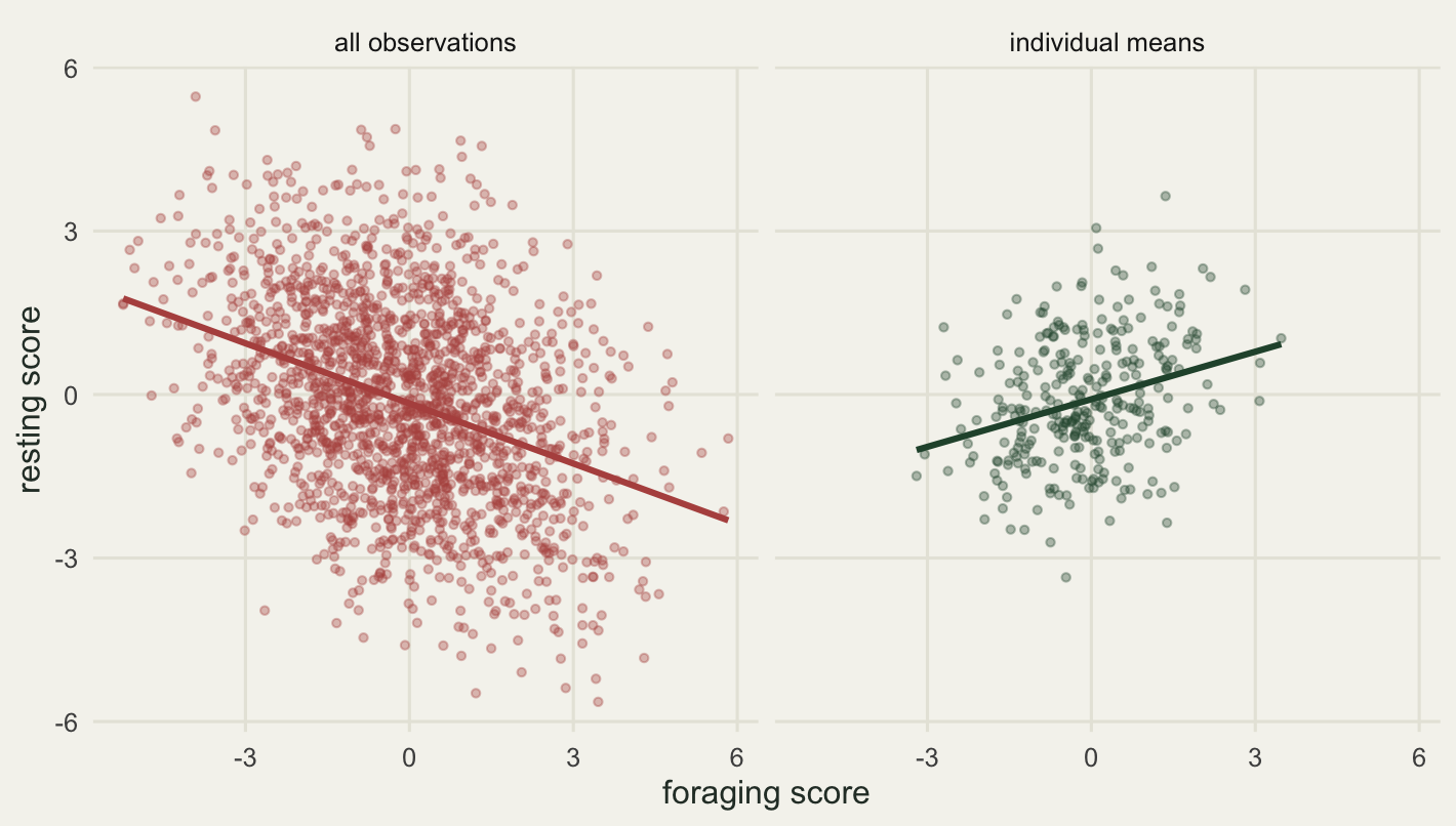
This is the picture most papers show, and this is the picture next to the picture they should have shown. The left panel is the raw scatter of all 1800 observations. It slopes down. Anyone looking at it concludes that foraging and resting trade off. The right panel is the same animals, one point each, and it slopes up.
There is a third number in that row worth pausing on. The correlation of the individual means is 0.2929, which has the right sign but is far below the estimated syndrome of 0.756. Averaging is an improvement over pooling, not a solution. An individual mean of 6 observations still carries residual noise, so the correlation of means is itself attenuated, by a factor that depends on how many repeats each animal received. This is why the right panel of the figure is a better picture but still not the estimate: the mixed model is what removes the remaining bias, because it estimates the variance of the residual noise and subtracts it rather than hoping it averaged away.
There is a quick diagnostic that costs nothing. Compute the correlation of individual means and the correlation of the within-individual deviations separately, which the partition helper already produces, and look at whether they have the same sign. If they do, the pooled correlation is a compromise and the worst that can happen is attenuation. If they differ in sign, the pooled correlation is a weighted difference of two opposing quantities and its value depends on the repeatabilities of the design rather than on the biology.
A practical consequence for reading the literature: a paper that reports the correlation of individual means with no mixed model is closer to right than one that pools, and both under-report the syndrome. The direction of the bias is always the same for the means version, so a mean-based syndrome estimate can be read as a lower bound on the magnitude when the within-individual correlation is weak, though not when it is strong and opposite in sign.
Fitting the bivariate model by hand
The moment estimator used so far is fast and unbiased for balanced designs, but it can return an among-individual matrix that is not positive definite, and it does not generalise to unbalanced data or extra fixed effects. The maximum likelihood fit does, so it is worth writing out.
It is also worth having the likelihood because it gives a likelihood ratio test for free. Fit the model once with the among-individual covariance free and once with the off-diagonal element fixed at zero, and twice the difference in log-likelihood is a test statistic for the null hypothesis of no syndrome. That is a better test than putting a p-value on the pooled correlation, which tests a different null.
Stack each individual’s observations trait by trait: the first k_rep entries are trait one at occasions one to k_rep, the next k_rep are trait two. The covariance matrix of that stacked vector has a Kronecker form. Every pair of occasions within an individual shares the same among-individual contribution, so the among-individual part is \(\Sigma_{\text{ind}} \otimes J_k\) where \(J_k\) is the all-ones matrix; the residual part contributes only on the diagonal in occasion, so it is \(\Sigma_{\text{e}} \otimes
I_k\). The whole thing is
\[V = \Sigma_{\text{ind}} \otimes J_k + \Sigma_{\text{e}} \otimes I_k\]
and it is the same \(V\) for every individual in a balanced design, so one Cholesky decomposition per likelihood evaluation serves all of them.
Both covariance matrices have to stay positive definite while optim wanders. The standard trick is to optimise the Cholesky factor instead of the matrix: write \(\Sigma = LL'\) with \(L\) lower triangular and the diagonal entries exponentiated. Three free numbers per matrix, six in total, and every point in that six-dimensional space maps to a valid pair of covariance matrices.
The exponential on the diagonal keeps the variances positive and the free off-diagonal entry of the factor can be any real number, so the parameter space is unconstrained and optim can use BFGS without any of the boundary trouble that constrained optimisers run into. The price is that the parameters are no longer the quantities of interest, so the covariance matrices have to be rebuilt from the factor before anything can be read off them.
The means drop out. Centring each column of the stacked data before optimising is exact rather than an approximation: with a balanced design and no covariates the generalised least squares estimate of a separate mean per column is that column’s ordinary average, whatever the covariance parameters are.
This is maximum likelihood rather than restricted maximum likelihood. REML would correct the variance components for the degrees of freedom used by the mean, which here is 10 out of 1500 observations, so the difference is small. It stops being small in a design with many fixed effects, and a real analysis with sex, age, trial order and observer in the model should use REML or a Bayesian fit rather than plain ML.
## three free numbers -> a 2x2 positive definite matrix, via a Cholesky factor
chol_pack <- function(p) {
  L <- matrix(0, 2, 2)
  L[1, 1] <- exp(p[1])
  L[2, 1] <- p[2]
  L[2, 2] <- exp(p[3])
  tcrossprod(L)
}

## n_ind by 2*k_rep matrix, trait-major columns
widen <- function(dat) {
  n_ind <- dat$n_ind
  k_rep <- dat$k_rep
  cbind(matrix(dat$y[, 1], n_ind, k_rep, byrow = TRUE),
        matrix(dat$y[, 2], n_ind, k_rep, byrow = TRUE))
}

neg_ll <- function(p, yw, k_rep) {
  SA <- chol_pack(p[1:3])
  SW <- chol_pack(p[4:6])
  V  <- kronecker(SA, matrix(1, k_rep, k_rep)) + kronecker(SW, diag(k_rep))
  ch <- tryCatch(chol(V), error = function(e) NULL)
  if (is.null(ch)) return(1e10)
  z <- backsolve(ch, t(yw), transpose = TRUE)
  0.5 * (nrow(yw) * 2 * sum(log(diag(ch))) + sum(z * z))
}

## moment estimates give the starting point
start_from <- function(S) {
  S <- S + diag(2) * 1e-6
  if (S[1, 1] <= 0 || S[2, 2] <= 0 || det(S) <= 0) {
    S <- diag(c(max(S[1, 1], 1e-3), max(S[2, 2], 1e-3)))
  }
  L <- t(chol(S))
  c(log(L[1, 1]), L[2, 1], log(L[2, 2]))
}

fit_bivariate <- function(dat) {
  yw  <- widen(dat)
  yw  <- sweep(yw, 2, colMeans(yw))
  mom <- partition(dat)
  p0  <- c(start_from(mom$among), start_from(mom$within))
  opt <- optim(p0, neg_ll, yw = yw, k_rep = dat$k_rep, method = "BFGS",
               control = list(maxit = 400, reltol = 1e-10))
  list(among = chol_pack(opt$par[1:3]),
       within = chol_pack(opt$par[4:6]),
       convergence = opt$convergence,
       logLik = -opt$value)
}
The likelihood is the multivariate normal one written efficiently. backsolve with the Cholesky factor turns the quadratic form into a sum of squares, so the whole data set contributes through one triangular solve of a 10 by 10 system and one matrix of the same size. There is no explicit inverse anywhere, and no loop over individuals.
Unbalanced data breaks the shortcut, not the method. If individuals have different numbers of observations, \(V\) has to be built per individual and the likelihood becomes a sum over individuals, which is slower but no harder to write. The Kronecker form still holds within each individual; only the block size changes. Missing one trait on some occasions is handled the same way, by dropping the corresponding rows and columns of \(V\) for that individual.
set.seed(20260730)

n_fit <- 300
k_fit <- 5
SA_true <- make_cov(1.0, 0.6,  0.55)
SW_true <- make_cov(2.0, 1.4, -0.30)

dat_fit <- sim_pair(n_fit, k_fit, SA_true, SW_true)
fit_ml  <- fit_bivariate(dat_fit)
fit_mom <- partition(dat_fit)

print(round(c(n_ind = n_fit, k_rep = k_fit,
              n_obs = n_fit * k_fit,
              system_size = 2 * k_fit,
              df_among = n_fit - 1,
              df_within = n_fit * (k_fit - 1),
              convergence = fit_ml$convergence,
              logLik = fit_ml$logLik), 4))
n_ind k_rep n_obs system_size df_among df_within
300.000 5.000 1500.000 10.000 299.000 1200.000
convergence logLik
0.000 -2518.412 print(round(c(ml_moment_gap = abs(cor_of(fit_ml$among) - cor_of(fit_mom$among))), 4))ml_moment_gap
0.001 print(data.frame(
quantity = c("among var 1", "among var 2", "among correlation",
"within var 1", "within var 2", "within correlation"),
truth = round(c(SA_true[1, 1], SA_true[2, 2], cor_of(SA_true),
SW_true[1, 1], SW_true[2, 2], cor_of(SW_true)), 4),
ml = round(c(fit_ml$among[1, 1], fit_ml$among[2, 2], cor_of(fit_ml$among),
fit_ml$within[1, 1], fit_ml$within[2, 2], cor_of(fit_ml$within)), 4),
moment = round(c(fit_mom$among[1, 1], fit_mom$among[2, 2], cor_of(fit_mom$among),
fit_mom$within[1, 1], fit_mom$within[2, 2],
cor_of(fit_mom$within)), 4))) quantity truth ml moment
1 among var 1 1.00 1.0003 1.0020
2 among var 2 0.60 0.5423 0.5445
3 among correlation 0.55 0.4396 0.4385
4 within var 1 2.00 1.9263 1.9407
5 within var 2 1.40 1.3500 1.3526
6 within correlation -0.30 -0.2775 -0.2743The optimiser converged (convergence is 0) on 300 individuals with 5 repeats each, 1500 observations in total. The within-individual quantities are recovered tightly: variances of 1.9263 and 1.35 against 2 and 1.4, correlation -0.2775 against -0.3. That is unsurprising: the within-individual matrix is estimated from 1200 degrees of freedom.
The among-individual side is the honest part of the output. The simulated syndrome is 0.55 and the fit returns 0.4396. That is not a coding error and it is not a bad optimiser: the maximum likelihood estimate and the moment estimate agree to 0.001, so both estimators are looking at the same information in the same data and both land in the same place. The among-individual matrix is estimated from 299 degrees of freedom, not 1500, and a correlation estimated from 300 units is simply not a precise thing.
Note also that the among-individual variance of the second trait comes back as 0.5423 against a simulated 0.6. The correlation error and the variance error are not independent: the correlation is a ratio, and the denominator is being estimated too.
The starting values come from the moment estimator, which matters more than it looks. Starting from an identity matrix, this likelihood has long flat valleys in the direction that trades among-individual variance against within-individual variance, and BFGS can spend a great many iterations crawling along one. Starting from a consistent estimate puts the optimiser close enough that convergence is quick and the reported log-likelihood of -2518.412 is reached from a sensible direction.
set.seed(20260731)

true_lv   <- c(-0.75, -0.45, -0.15, 0.15, 0.45, 0.75)
n_rec     <- 250
k_rec     <- 4
per_level <- 5

rec <- NULL
for (r_target in true_lv) {
  for (b in seq_len(per_level)) {
    sa <- make_cov(1.0, 0.6, r_target)
    sw <- make_cov(2.0, 1.4, -0.30)
    dd <- sim_pair(n_rec, k_rec, sa, sw)
    ff <- fit_bivariate(dd)
    rec <- rbind(rec, data.frame(truth = r_target,
                                 estimate = cor_of(ff$among),
                                 conv = ff$convergence))
  }
}

rec_span <- sapply(split(rec$estimate, rec$truth), function(v) diff(range(v)))

print(round(c(simulated_levels = true_lv), 4))
simulated_levels1 simulated_levels2 simulated_levels3 simulated_levels4
-0.75 -0.45 -0.15 0.15
simulated_levels5 simulated_levels6
0.45 0.75 print(round(rec_span, 4)) -0.75 -0.45 -0.15 0.15 0.45 0.75
0.1028 0.1802 0.0890 0.2441 0.3535 0.2272 print(round(c(fits = nrow(rec), n_ind = n_rec, k_rep = k_rec,
per_level = per_level,
bias = mean(rec$estimate - rec$truth),
rmse = sqrt(mean((rec$estimate - rec$truth)^2)),
max_abs_error = max(abs(rec$estimate - rec$truth)),
non_converged = sum(rec$conv != 0)), 4)) fits n_ind k_rep per_level bias
30.0000 250.0000 4.0000 5.0000 0.0027
rmse max_abs_error non_converged
0.0803 0.2368 0.0000 30 fits, 5 at each of 6 simulated values of the syndrome, each on 250 individuals with 4 repeats. Every one converged (non_converged is 0). The mean error is 0.0027, so the estimator is close to unbiased across this range. The root mean squared error is 0.0803 and the worst single fit missed by 0.2368.
ggplot(rec, aes(truth, estimate)) +
  geom_abline(intercept = 0, slope = 1,
              colour = te_pal$sage, linewidth = 0.6, linetype = "22") +
  geom_point(aes(colour = "single fit", shape = "single fit"), size = 2.2, alpha = 0.85) +
  stat_summary(aes(colour = "mean of five fits", shape = "mean of five fits"),
               fun = mean, geom = "point", size = 3.2) +
  scale_colour_manual(values = c("single fit" = te_pal$clay,
                                 "mean of five fits" = te_pal$forest),
                      breaks = c("single fit", "mean of five fits"), name = NULL) +
  scale_shape_manual(values = c("single fit" = 16, "mean of five fits" = 17),
                     breaks = c("single fit", "mean of five fits"), name = NULL) +
  labs(x = "simulated among-individual correlation",
       y = "estimated among-individual correlation") +
  theme_te()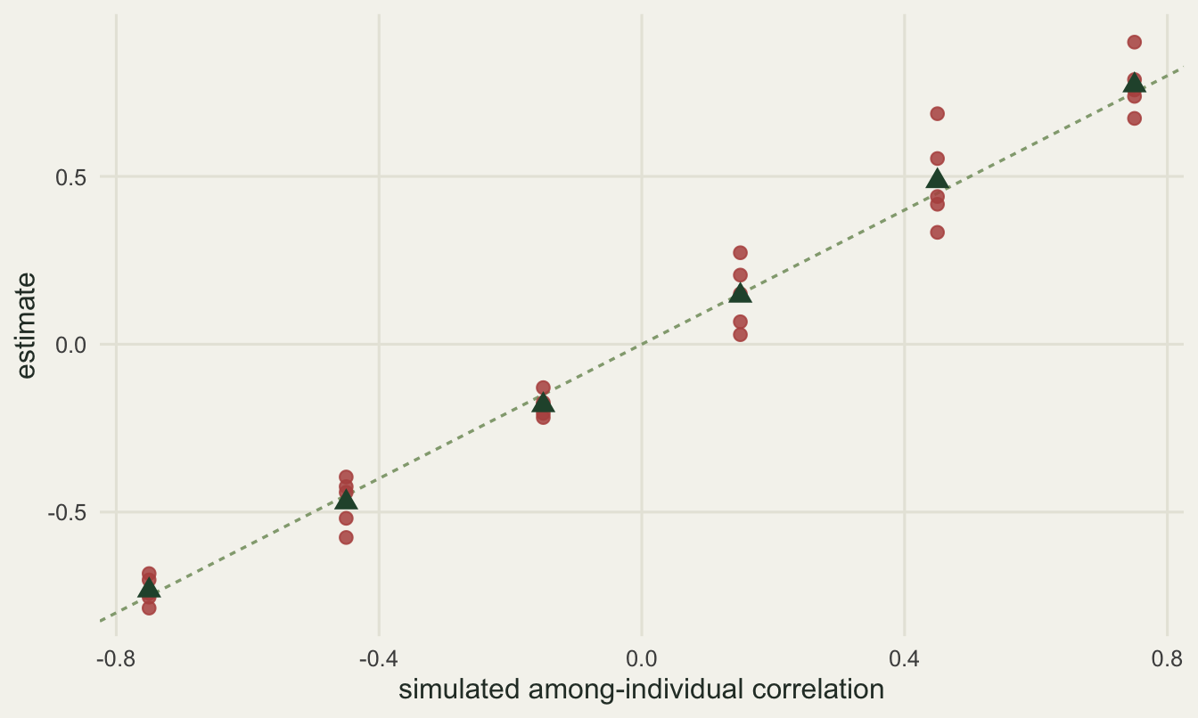
The green triangles sit on the dotted line, which is the definition of an unbiased estimator and the thing the section set out to check. The red points are the reason the next section exists. With 250 individuals, a design most behavioural studies would consider generous, a single fit can land 0.2368 away from the truth. That is the difference between reporting a moderate syndrome and reporting no syndrome at all.
The sampling variance of a correlation scales roughly with \((1 - r^2)^2\), so estimates near zero should be the noisiest in absolute terms. The figure does not show that, and it is worth saying so rather than reading the expected pattern into it. The vertical span of each cluster, printed above, is smallest at a simulated -0.15 at 0.0890, one of the two levels closest to zero, and largest at 0.45 at 0.3535. What the figure does show, that every cluster on the positive side is taller than every one on the negative side, is not a property of the estimator either. Five fits per level put a Monte Carlo error on the spread itself that swamps the effect the theory predicts. The theoretical point still stands, and it is the inconvenient one: the interesting question is usually whether the syndrome differs from zero, and zero is where a correlation is hardest to pin down.
Five fits per level is a small number and it is deliberately small: the point of this figure is to show the spread of individual fits, not to estimate the sampling distribution precisely. The next section does the latter properly with 500 replicates per design, using the moment estimator so that the cost stays reasonable.
How precisely can a syndrome be measured?
The design question every behavioural study faces is how to spend a fixed number of observations. More individuals with fewer repeats each, or fewer individuals measured more often? The advice one usually hears is that among-individual quantities need individuals, so put the effort there.
To measure this rather than assert it, simulate many data sets at each design, estimate the syndrome in each, and report the width of the interval containing the middle 95% of the estimates. The moment estimator is used here rather than the likelihood fit, because the previous section showed the two agree to 0.001 on the same data, and the moment estimator is fast enough to run hundreds of times per cell.
The interval is measured from repeated simulation rather than read off the Hessian of the likelihood. That is a choice. The Hessian gives an asymptotic standard error on the Cholesky scale which then has to be pushed through the transformation to the correlation, and correlations near the boundary are exactly where that approximation is worst. Simulating the design and looking at the spread of estimates answers the design question directly and does not assume normality of the estimator.
set.seed(20260801)

r_from_sim <- function(n_ind, k_rep, S_among, S_within) {
  prt <- partition(sim_pair(n_ind, k_rep, S_among, S_within))
  if (prt$among[1, 1] <= 0 || prt$among[2, 2] <= 0) return(NA_real_)
  cor_of(prt$among)
}

n_boot     <- 500
rep_typ    <- 0.37
r_true_pre <- 0.50
SA_pre <- make_cov(1, 1, r_true_pre)
SW_pre <- make_cov((1 - rep_typ) / rep_typ, (1 - rep_typ) / rep_typ, 0)

pre <- expand.grid(n_ind = c(50, 100, 200, 400), k_rep = c(2, 4, 8))
pre$width <- NA_real_
pre$undefined <- NA_real_

for (i in seq_len(nrow(pre))) {
  v <- replicate(n_boot, r_from_sim(pre$n_ind[i], pre$k_rep[i], SA_pre, SW_pre))
  pre$undefined[i] <- mean(is.na(v) | abs(v) > 1)
  v <- pmax(-1, pmin(1, v[!is.na(v)]))
  pre$width[i] <- as.numeric(diff(quantile(v, c(0.025, 0.975))))
}

pre$n_obs <- pre$n_ind * pre$k_rep

print(round(c(replicates = n_boot, r_simulated = r_true_pre,
              repeatability = rep_typ, interval_pct = 95), 4))
replicates r_simulated repeatability interval_pct
500.00 0.50 0.37 95.00 print(round(pre, 4)) n_ind k_rep width undefined n_obs
1 50 2 1.0321 0.074 100
2 100 2 0.8457 0.018 200
3 200 2 0.5512 0.002 400
4 400 2 0.3748 0.000 800
5 50 4 0.7119 0.002 200
6 100 4 0.5167 0.000 400
7 200 4 0.3344 0.000 800
8 400 4 0.2330 0.000 1600
9 50 8 0.5517 0.000 400
10 100 8 0.4171 0.000 800
11 200 8 0.2722 0.000 1600
12 400 8 0.1901 0.000 3200print(round(c(cost_extra_individuals = pre$n_obs[4] - pre$n_obs[1],
gain_extra_individuals = pre$width[1] - pre$width[4],
cost_extra_repeats = pre$n_obs[9] - pre$n_obs[1],
gain_extra_repeats = pre$width[1] - pre$width[9]), 4))cost_extra_individuals gain_extra_individuals cost_extra_repeats
700.0000 0.6573 300.0000
gain_extra_repeats
0.4804 The simulated syndrome is 0.5 and both repeatabilities are 0.37, near the behavioural average. Each cell is 500 replicate data sets.
Start with the top-left corner, 50 individuals measured 2 times. The 95% interval for the syndrome is 1.0321 wide. The parameter can only live between minus one and one, so an interval of that width is close to no information at all, and 0.074 of the replicates produced an among-individual matrix with a non-positive variance or a correlation outside the legal range, which in a real analysis would appear as a boundary estimate or a convergence failure.
The bottom-right corner, 400 individuals measured 8 times, gives a width of 0.1901. That is a usable estimate, and it costs 3200 observations. A commonly seen design in the literature, 100 individuals measured 2 times, gives 0.8457: an estimate of 0.5 with an interval of that width tells you almost nothing beyond the sign, and only if you are lucky about the sign.
The undefined column is not a nuisance either. At 50 individuals and 2 repeats, 0.074 of replicates failed to return a legal among-individual correlation, either from a variance at or below zero or from a correlation outside minus one to one, which is what a boundary estimate looks like when it happens in real software. A fitting routine that reports a correlation of exactly one, or refuses to converge, is usually telling you that the design cannot support the estimate rather than that the code is broken.
ggplot(pre, aes(n_ind, width,
                colour = factor(k_rep), shape = factor(k_rep))) +
  geom_line(linewidth = 0.8) +
  geom_point(size = 2.6) +
  scale_x_continuous(breaks = c(50, 100, 200, 400)) +
  scale_colour_manual(values = c(te_pal$clay, te_pal$gold, te_pal$forest),
                      name = "repeats per individual") +
  scale_shape_manual(values = c(16, 17, 15),
                     name = "repeats per individual") +
  labs(x = "number of individuals", y = "width of 95% interval") +
  theme_te()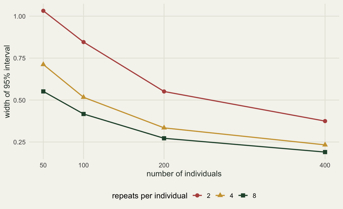
Both axes of effort work, which the figure shows plainly, but they are not interchangeable. Going from 50 to 400 individuals at 2 repeats takes the width from 1.0321 to 0.3748, and costs 700 extra observations. Going from 2 to 8 repeats at 50 individuals takes it from 1.0321 to 0.5517, and costs 300 extra observations. The second move is a smaller gain but a far cheaper one, which is not what the standard advice predicts.
The clean way to settle it is to hold the number of observations fixed and vary how they are spread.
set.seed(20260802)

budget  <- 1200
designs <- data.frame(n_ind = c(600, 300, 200, 150, 100, 60),
                      k_rep = c(2, 4, 6, 8, 12, 20))

bud <- NULL
for (rr in c(0.15, 0.37, 0.65)) {
  sa <- make_cov(1, 1, r_true_pre)
  sw <- make_cov((1 - rr) / rr, (1 - rr) / rr, 0)
  w  <- numeric(nrow(designs))
  for (i in seq_len(nrow(designs))) {
    v <- replicate(n_boot, r_from_sim(designs$n_ind[i], designs$k_rep[i], sa, sw))
    v <- pmax(-1, pmin(1, v[!is.na(v)]))
    w[i] <- as.numeric(diff(quantile(v, c(0.025, 0.975))))
  }
  bud <- rbind(bud, data.frame(repeatability = rr,
                               n_ind = designs$n_ind,
                               k_rep = designs$k_rep,
                               width = round(w, 4)))
}

best <- do.call(rbind, lapply(split(bud, bud$repeatability), function(s) {
  data.frame(repeatability = s$repeatability[1],
             best_k = s$k_rep[which.min(s$width)],
             best_width = min(s$width),
             width_at_k2 = s$width[s$k_rep == 2],
             penalty_for_k2 = round(s$width[s$k_rep == 2] - min(s$width), 4))
}))

print(round(c(budget_obs = budget, replicates = n_boot,
              r_simulated = r_true_pre), 4))
budget_obs replicates r_simulated
1200.0 500.0 0.5 print(bud) repeatability n_ind k_rep width
1 0.15 600 2 0.8847
2 0.15 300 4 0.5718
3 0.15 200 6 0.4990
4 0.15 150 8 0.5146
5 0.15 100 12 0.4775
6 0.15 60 20 0.5660
7 0.37 600 2 0.3133
8 0.37 300 4 0.2829
9 0.37 200 6 0.3026
10 0.37 150 8 0.2973
11 0.37 100 12 0.3621
12 0.37 60 20 0.4616
13 0.65 600 2 0.1668
14 0.65 300 4 0.2032
15 0.65 200 6 0.2303
16 0.65 150 8 0.2520
17 0.65 100 12 0.3203
18 0.65 60 20 0.4038print(best) repeatability best_k best_width width_at_k2 penalty_for_k2
0.15 0.15 12 0.4775 0.8847 0.4072
0.37 0.37 4 0.2829 0.3133 0.0304
0.65 0.65 2 0.1668 0.1668 0.0000Every design in that table costs 1200 observations. The answer is not the one the standard advice gives, and it is not one answer.
At a repeatability of 0.65, the usual advice is right: the widest possible design wins, 600 individuals measured 2 times gives a width of 0.1668, and every step towards fewer individuals with more repeats makes it worse.
At a repeatability of 0.37, which is where most behavioural traits actually sit, the best design in the table uses 4 repeats per individual and gives a width of 0.2829, against 0.3133 for the two-repeat design. The penalty for following the standard advice is 0.0304 of interval width, which is modest but real, and it goes the opposite way to what one is normally told.
At a repeatability of 0.15 the standard advice is clearly wrong. The best design in the table uses 12 repeats per individual for a width of 0.4775, while the maximum-individuals design gives 0.8847. The penalty for spreading the same 1200 observations across as many animals as possible is 0.4072 of interval width, close to doubling it.
The mechanism is not mysterious once the number is in front of you. The among-individual correlation is a correlation between quantities that are themselves estimated. With few repeats and low repeatability, each individual’s mean is such a poor estimate of that individual’s true tendency that adding more individuals adds mostly noise. Repeats buy reliability per individual, individuals buy sample size, and the exchange rate depends on the repeatability. Above roughly the value where the estimated individual mean becomes a decent measurement, individuals win; below it, repeats do.
Two limits explain the shape of the table. With one repeat per individual the model is not identified at all, because there is no within-individual variation to estimate. With an infinite number of repeats each individual mean is exact and the width settles at the width of an ordinary correlation on that many individuals, which cannot be beaten. Between those, the effective sample size behaves like the number of individuals discounted by how reliable each individual mean is, and the discount is severe when repeatability is low.
The practical form of the rule: estimate the repeatability of both traits first, from a pilot or from the literature, and only then decide how to spend the observations. If the repeatabilities are around 0.15, plan for repeats in the range this table found best rather than for the largest possible number of animals. A study that measures 600 animals twice each because that was the advice has, at low repeatability, thrown away roughly half the precision available in its own budget.
What to take away
A behavioural syndrome is a correlation between individual means, and the correlation you get by pooling all observations is a different quantity: a mixture of the among-individual and within-individual correlations, weighted by \(\sqrt{R_1 R_2}\) and \(\sqrt{(1-R_1)(1-R_2)}\). When the within-individual correlation is zero the pooled version is an attenuated copy, which is merely conservative. When the within-individual correlation is strong and opposite in sign, the pooled version can reverse: a simulated syndrome of 0.7 produced a pooled correlation of -0.363, and a simulated syndrome of -0.7 produced a pooled correlation of 0.3346. Both come from time-budget or state effects that are ordinary in behavioural data.
Fitting the bivariate model is not hard. Six free numbers, two Cholesky factors, one optim call, and the estimator recovered the simulated value with a mean error of 0.0027 across 30 fits. What is hard is precision. With 250 individuals and 4 repeats the worst of those 30 fits was off by 0.2368, and at a realistic repeatability of 0.37 a design of 100 individuals by 2 repeats gave a 95% interval 0.8457 wide. Reporting a syndrome without an interval on it is reporting a number whose sign is often not established.
The honest limit is what the estimate is an estimate of. A syndrome measured this way is a statistical association among individual means, in one population, in one set of contexts, over the period the measurements were taken. It is not evidence of a genetic correlation, of a physiological constraint, or of any shared mechanism; a permanent environmental effect such as territory quality or early nutrition produces exactly the same among-individual covariance as a pleiotropic gene, and the design here cannot tell them apart. Measure the same individuals in a different context, or the same species in a different population, and the number can change or reverse without anything being wrong with either measurement. The model separates among-individual from within-individual covariation, which is a real and necessary separation, and it stops there.
What to report, then: both correlations, the two repeatabilities, and the number of individuals and repeats behind them. That is four numbers and a design, and it is enough for a reader to reconstruct the identity and see for themselves how much of the pooled correlation is the syndrome. A paper that gives only the pooled value has not reported the syndrome at all, and a paper that gives only the among-individual value has hidden the within-individual biology that may be the more interesting half.
References
Sih A, Bell A, Johnson JC 2004 Trends in Ecology and Evolution 19(7):372-378 (10.1016/j.tree.2004.04.009)
Reale D, Reader SM, Sol D, McDougall PT, Dingemanse NJ 2007 Biological Reviews 82(2):291-318 (10.1111/j.1469-185X.2007.00010.x)
Bell AM, Hankison SJ, Laskowski KL 2009 Animal Behaviour 77(4):771-783 (10.1016/j.anbehav.2008.12.022)
Nakagawa S, Schielzeth H 2010 Biological Reviews 85(4):935-956 (10.1111/j.1469-185X.2010.00141.x)
Hadfield JD 2010 Journal of Statistical Software 33(2):1-22 (10.18637/jss.v033.i02)
Dingemanse NJ, Dochtermann NA 2013 Journal of Animal Ecology 82(1):39-54 (10.1111/1365-2656.12013)
Lynch M, Walsh B 1998 Genetics and Analysis of Quantitative Traits (ISBN 978-0-87893-481-2)