library(ggplot2)

te_pal <- list(forest = "#275139", green = "#2f8f63", sage = "#93a87f",
               clay = "#b5534e", gold = "#cda23f", line = "#dad9ca",
               ink = "#16241d", paper = "#f5f4ee")

theme_te <- function() {
  theme_minimal(base_size = 12) +
    theme(panel.grid.minor = element_blank(),
          panel.grid.major = element_line(colour = "#e7e6dc"),
          plot.background = element_rect(fill = "#f5f4ee", colour = NA),
          panel.background = element_rect(fill = "#f5f4ee", colour = NA),
          plot.title = element_text(face = "bold", colour = te_pal$ink),
          axis.title = element_text(colour = "#2c3a31"),
          legend.position = "bottom")
}

## fixed-decimal formatter so quoted values match the printed tables
fmt <- function(x, d = 4) sprintf(paste0("%.", d, "f"), x)Adjusted repeatability in R
R
behaviour
mixed models
repeatability
ecology tutorial
Repeatability shifts meaning once a model carries fixed effects. Hand-coded REML in R separates the raw, adjusted and enhanced versions and measures the gap.
The exploration trials happen in a plywood box behind the ringing hut. A great tit comes out of the cloth bag, the sliding door goes up, and for two minutes one person counts how many of the five artificial trees the bird lands on. The number goes on a card, the bird goes back out of the window, and the box gets wiped down for the next one. Sixty birds, six trials each, spread across two winters and the breeding seasons between them.
The point of all that repetition is a single number. If the same bird tends to score high every time and another bird tends to score low, then exploration is a property of birds and not just of mornings, and it makes sense to ask what else it predicts. That number is the repeatability: the share of the total variance in the score that sits among birds rather than within them. It is the first thing anyone reports from a design like this, and it is the number that gets pulled into meta-analyses and into power calculations for the next study.
The trouble starts when you put anything else in the model. Scores are higher in the breeding season than in midwinter, so you fit season as a fixed effect, and now the model has three quantities in it that all get called repeatability in print. They differ in which fit supplies the numerator and in what goes into the denominator, they can be a factor of nearly three apart on the same data, and papers report them without always saying which one they computed. A number copied out of a table into a meta-analysis is therefore not necessarily comparable with the number two rows below it.
This post builds the variance components by hand, computes all three versions of R on one simulated data set, and measures how far apart they land under two designs that differ only in where the season effect sits. It then puts confidence intervals on R two ways and measures whether either of them covers.
One thing this post is not about. This blog already has Checking a measurement-error correction, which computes an intraclass correlation from repeated readings of the same quantity and uses it as a reliability, then corrects a regression slope for the dilution that unreliability causes. There the within-unit variation is the instrument wobbling, and it is a nuisance to be removed. Here the within-individual variation is real: the bird genuinely behaves differently on different mornings, and nobody wants that scrubbed out. The algebra of the intraclass correlation is the same in both places, but the estimand is not, and the two posts answer different questions.
Splitting one variance two ways
The model behind every repeatability is the one-way random effects model. Write \(y_{ij}\) for the \(j\)th score of individual \(i\), and let
\[y_{ij} = \mu + a_i + e_{ij}, \qquad a_i \sim N(0, \sigma^2_a), \qquad e_{ij} \sim N(0, \sigma^2_e).\]
The repeatability is \(R = \sigma^2_a / (\sigma^2_a + \sigma^2_e)\). Everything in this post is an argument about which variances belong in that ratio, so the first job is to get \(\sigma^2_a\) and \(\sigma^2_e\) out of the data.
There are two classical routes. The moment route reads them off the analysis of variance table: the within-individual mean square estimates \(\sigma^2_e\) directly, and the among-individual mean square has expectation \(\sigma^2_e + n_0 \sigma^2_a\), where \(n_0\) is a design constant that equals the number of repeats per individual when the design is balanced and something slightly smaller when it is not. Subtract and divide. The likelihood route maximises the restricted likelihood, which is the likelihood of the residual contrasts left after the fixed part has been projected out. Both are written out below in base R.
The restricted likelihood needs the inverse and the determinant of \(V = \sigma^2_a ZZ' + \sigma^2_e I\), and for a single random intercept both have closed forms that never build the matrix. Factor out \(\sigma^2_e\) and let \(\lambda = \sigma^2_a / \sigma^2_e\). Then \(M = \lambda ZZ' + I\) is block diagonal, its determinant is the product of \(1 + \lambda n_i\) over individuals, and multiplying a vector by \(M^{-1}\) means subtracting a shrunken group sum from every element. That leaves one free parameter to optimise over, because the residual variance can be profiled out analytically, so optim only has to search a line.
Restricted rather than plain maximum likelihood matters here, and it will matter again later in the post. Plain maximum likelihood treats the fixed effects as known when it estimates the variances, so it charges the variance components for degrees of freedom that were actually spent on the mean. The restricted version works with contrasts that carry no information about the fixed part at all, which is exactly why it pays no such charge. On a model with an intercept and nothing else the difference is a factor close to one; on a model with thirty fixed levels it is not.
## moment estimator from the one-way mean squares
anova_vc <- function(yv, idv) {
  ids <- sort(unique(idv)); k <- length(ids); N <- length(yv)
  ni  <- as.vector(tapply(yv, idv, length)[as.character(ids)])
  gmn <- as.vector(tapply(yv, idv, mean)[as.character(ids)])
  pos <- match(idv, ids)
  msa <- sum(ni * (gmn - mean(yv))^2) / (k - 1)
  msw <- sum((yv - gmn[pos])^2) / (N - k)
  n0  <- (N - sum(ni^2) / N) / (k - 1)
  c(among = max((msa - msw) / n0, 0), within = msw,
    msa = msa, msw = msw, n0 = n0)
}

## multiply a vector or matrix by the inverse of M = lambda ZZ' + I
minv <- function(vv, pos, wt) {
  if (is.matrix(vv)) {
    gs <- rowsum(vv, pos)
    vv - wt[pos] * gs[pos, , drop = FALSE]
  } else {
    gs <- as.vector(rowsum(vv, pos))
    vv - wt[pos] * gs[pos]
  }
}

## profiled REML for y = X b + Z a + e with one random intercept
reml_fit <- function(yv, X, idv) {
  ids <- sort(unique(idv)); N <- length(yv); p <- ncol(X)
  pos <- match(idv, ids)
  ni  <- as.vector(table(pos))
  core <- function(lg) {
    lam <- exp(lg); wt <- lam / (1 + lam * ni)
    MiX <- minv(X, pos, wt); Miy <- minv(yv, pos, wt)
    A  <- crossprod(X, MiX); ch <- chol(A)
    bh <- backsolve(ch, backsolve(ch, crossprod(X, Miy), transpose = TRUE))
    rr <- as.vector(yv - X %*% bh)
    qq <- sum(rr * minv(rr, pos, wt))
    s2e <- qq / (N - p)
    list(dev = sum(log(1 + lam * ni)) + 2 * sum(log(diag(ch))) +
                (N - p) * log(s2e),
         s2e = s2e, bh = as.vector(bh))
  }
  op  <- optim(0, function(lg) core(lg)$dev, method = "Brent",
               lower = -12, upper = 8)
  fin <- core(op$par); lam <- exp(op$par)
  list(among = lam * fin$s2e, within = fin$s2e, bta = fin$bh,
       fixed = as.vector(X %*% fin$bh))
}
Now simulate a balanced design and run both estimators on it. The true among-individual variance and the true residual variance are set to values that give a repeatability a little above one third, which is roughly where behavioural repeatabilities in birds tend to sit.
set.seed(20260727)
s2a_t <- 0.60; s2e_t <- 1.00
nind1 <- 40; nrep1 <- 5
id_b <- rep(seq_len(nind1), each = nrep1)
y_b  <- rnorm(nind1, 0, sqrt(s2a_t))[id_b] +
        rnorm(nind1 * nrep1, 0, sqrt(s2e_t))

ab <- anova_vc(y_b, id_b)
rb <- reml_fit(y_b, matrix(1, length(y_b), 1), id_b)

print(round(c(true_among = s2a_t, true_within = s2e_t,
              true_R = s2a_t / (s2a_t + s2e_t),
              n_individuals = nind1, n_per_individual = nrep1,
              n_obs = length(y_b),
              anova_among = ab[["among"]], reml_among = rb$among,
              anova_within = ab[["within"]], reml_within = rb$within,
              gap_among = abs(ab[["among"]] - rb$among),
              gap_within = abs(ab[["within"]] - rb$within)), 6))
true_among true_within true_R n_individuals
0.600000 1.000000 0.375000 40.000000
n_per_individual n_obs anova_among reml_among
5.000000 200.000000 0.699793 0.699793
anova_within reml_within gap_among gap_within
0.895048 0.895048 0.000000 0.000000 The two estimators return the same numbers to six decimal places. The among-individual variance is 0.699793 by both routes and the residual variance is 0.895048 by both routes, so the gaps are 0.000000 and 0.000000.
This is not luck. For a balanced one-way model with nothing but an intercept in the fixed part, the restricted likelihood is maximised exactly at the moment solution whenever that solution is positive, and the two methods are the same estimator wearing different clothes. Both land above the true among-individual variance of 0.600000, which is the sort of error 40 individuals buys you: the standard error on a variance component is governed by the number of individuals, not by the number of observations, and forty is not many.
Unbalance breaks the equivalence. Give another 40 birds wildly different numbers of trials, from two up to twelve, and fit both estimators again.
set.seed(20260728)
nu   <- rep(c(2, 3, 9, 12), length.out = nind1)
id_u <- rep(seq_len(nind1), times = nu)
y_u  <- rnorm(nind1, 0, sqrt(s2a_t))[id_u] +
        rnorm(length(id_u), 0, sqrt(s2e_t))

au <- anova_vc(y_u, id_u)
ru <- reml_fit(y_u, matrix(1, length(y_u), 1), id_u)

print(round(c(n_obs = length(y_u), min_trials = min(nu), max_trials = max(nu),
              mean_trials = length(y_u) / nind1, n0 = au[["n0"]],
              anova_among = au[["among"]], reml_among = ru$among,
              anova_within = au[["within"]], reml_within = ru$within,
              anova_R = au[["among"]] / (au[["among"]] + au[["within"]]),
              reml_R = ru$among / (ru$among + ru$within)), 4))
n_obs min_trials max_trials mean_trials n0 anova_among
260.0000 2.0000 12.0000 6.5000 6.4320 1.2842
reml_among anova_within reml_within anova_R reml_R
1.0734 1.0751 1.0667 0.5443 0.5016 With 260 observations and trial counts running from 2 to 12, the design constant \(n_0\) comes out at 6.4320, which sits below the average of 6.50 trials per bird because \(n_0\) penalises spread in the group sizes. The two estimators now disagree, and not by a rounding error: the moment estimate of the among-individual variance is 1.2842 against 1.0734 from REML. The repeatabilities that follow are 0.5443 and 0.5016.
The reason is that the moment estimator gives every individual the same weight through the single constant \(n_0\), while REML weights an individual by how much information it carries, so a bird with twelve trials counts for more than a bird with two. On unbalanced data the moment estimator is still unbiased but it is no longer efficient, and its answer wanders further from the truth on any particular data set. Papers that report a repeatability computed from mean squares on a badly unbalanced design are not doing anything illegal, but they are leaving information on the floor, and with heavy unbalance the moment estimator also produces negative variance estimates often enough to be a nuisance.
Everything after this section uses REML, and every design after this section is balanced, which removes one source of argument from the comparisons that follow. Balance is not realistic for field data, but it is the right choice for a post whose subject is the difference between three definitions: if the designs were unbalanced as well, you would not know which part of a gap came from the definition and which from the estimator.
Three quantities that all get called repeatability
Now add the season. Sixty birds, six trials each. In the first design each bird is measured three times in one season and three times in the other, so the season contrast lives inside every bird’s record. In the second design each bird is measured six times in a single season, and half the birds belong to each season, so the season contrast lives entirely between birds. The underlying birds are identical in the two designs: the same individual effects, the same residuals, the same season slope. Only the allocation changes.
Both allocations happen in real projects, and usually by accident rather than by choice. The first is what you get when the fieldwork runs continuously and everything gets caught in both halves of the year. The second is what you get when a site is worked hard for one season, then a different site the next, or when birds recruit and disappear fast enough that most individuals only ever overlap with one sampling window. The design decision that produces the difference is often nobody’s decision at all.
Given a fitted model with a fixed effect in it, three ratios are in circulation.
The raw or agreement repeatability leaves the fixed effect out of the model altogether and asks how much of the total observed variance sits among individuals. It answers a question about the data as they came in: if you pick two scores from the same bird and two scores from different birds, how much more alike are the first pair?
The adjusted or conditional repeatability fits the fixed effect, then forms the ratio from the two remaining variance components. The fixed effect is gone from both the top and the bottom of the fraction, so it answers a question about birds compared within a season: given the season, how much of what is left sits among individuals?
The enhanced or marginal version fits the fixed effect, keeps the among-individual variance on top, and puts the variance explained by the fixed effect back into the denominator alongside the residual. It answers the raw question, but with the among-individual variance estimated from the adjusted model rather than the unadjusted one.
bta_t <- 2.0; nind <- 60; nrep <- 6
idv <- rep(seq_len(nind), each = nrep)
x_w <- rep(c(0, 0, 0, 1, 1, 1), times = nind)            # season within bird
x_b <- rep(rep(c(0, 1), each = nind / 2), each = nrep)   # season between birds

three_r <- function(yv, idv, xv) {
  f0 <- reml_fit(yv, matrix(1, length(yv), 1), idv)
  f1 <- reml_fit(yv, cbind(1, xv), idv)
  s2f <- stats::var(f1$fixed)
  c(raw       = f0$among / (f0$among + f0$within),
    adjusted  = f1$among / (f1$among + f1$within),
    enhanced  = f1$among / (f1$among + f1$within + s2f),
    among_raw = f0$among, within_raw = f0$within,
    among_adj = f1$among, within_adj = f1$within,
    fixed_var = s2f, slope = f1$bta[2])
}

set.seed(20260729)
a_i   <- rnorm(nind, 0, sqrt(s2a_t))
e_ij  <- rnorm(nind * nrep, 0, sqrt(s2e_t))
y_win <- a_i[idv] + bta_t * x_w + e_ij
y_btw <- a_i[idv] + bta_t * x_b + e_ij

one_w <- three_r(y_win, idv, x_w)
one_b <- three_r(y_btw, idv, x_b)

sel_fig  <- c(1:5, 31:35)
step_mid <- vapply(sel_fig, function(i) {
  v <- y_win[idv == i]; v[4] - v[3]
}, numeric(1))

print(round(c(n_individuals = nind, n_per_individual = nrep,
              n_obs = nind * nrep, true_slope = bta_t,
              n_shown_in_figure = length(sel_fig),
              n_shown_stepping_up = sum(step_mid > 0),
              largest_step_down = min(step_mid)), 4))
n_individuals n_per_individual n_obs true_slope
60.0000 6.0000 360.0000 2.0000
n_shown_in_figure n_shown_stepping_up largest_step_down
10.0000 9.0000 -2.3026 print(round(one_w, 4)) raw adjusted enhanced among_raw within_raw among_adj within_adj
0.1366 0.3801 0.2201 0.3932 2.4856 0.6349 1.0355
fixed_var slope
1.2147 2.2012 print(round(one_b, 4)) raw adjusted enhanced among_raw within_raw among_adj within_adj
0.5991 0.3820 0.2477 1.5604 1.0442 0.6453 1.0442
fixed_var slope
0.9161 1.9116 print(round(c(ratio_within = one_w[["adjusted"]] / one_w[["raw"]],
ratio_between = one_b[["adjusted"]] / one_b[["raw"]]), 4)) ratio_within ratio_between
2.7828 0.6376 keep <- idv %in% sel_fig
occ <- rep(seq_len(nrep), times = nind)
traj <- data.frame(
occasion = rep(occ[keep], 2),
value = c(y_win[keep], y_btw[keep]),
ind = factor(rep(idv[keep], 2)),
season = factor(c(x_w[keep], x_b[keep]),
labels = c("season 1", "season 2")),
design = factor(rep(c("W", "B"), each = sum(keep)), levels = c("W", "B"),
labels = c("season varies within individuals",
"season varies between individuals")))
ggplot(traj, aes(occasion, value)) +
geom_line(aes(group = ind), colour = "#8c8b7e", linewidth = 0.9) +
geom_line(aes(group = interaction(ind, season), colour = season),
linewidth = 1.1) +
geom_point(aes(colour = season, shape = season), size = 2) +
facet_wrap(~design) +
scale_colour_manual(values = c(te_pal$forest, te_pal$clay)) +
scale_shape_manual(values = c(16, 17)) +
scale_x_continuous(breaks = 1:6) +
labs(x = "measurement occasion", y = "exploration score",
colour = NULL, shape = NULL) +
theme_te()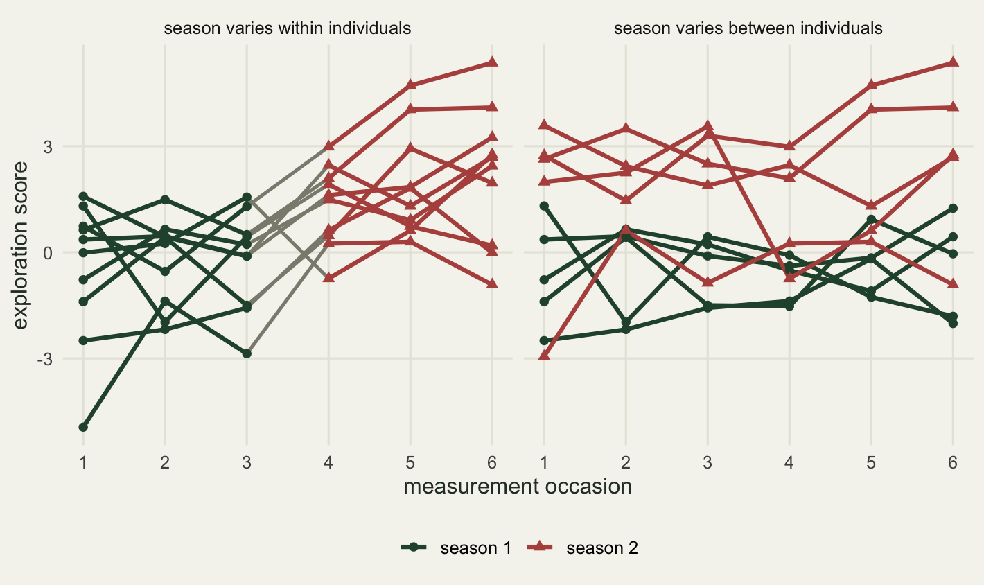
Read the two blocks of output against each other. In the within-individual design the raw repeatability is 0.1366 and the adjusted repeatability is 0.3801, a ratio of 2.7828. In the between-individual design the raw repeatability is 0.5991 and the adjusted repeatability is 0.3820, a ratio of 0.6376. The same adjustment, applied to data generated from the same individual effects and the same residuals, multiplies the raw value by 2.7828 in one design and by 0.6376 in the other.
The variance components say why. In the within-individual design the unadjusted residual variance is 2.4856 against 1.0355 once season is fitted, because the season step is inside each bird’s record and the unadjusted model has nowhere to put it except the residual. In the between-individual design the unadjusted among-individual variance is 1.5604 against 0.6453 once season is fitted, because there the season step is a difference between birds and the unadjusted model files it under individual identity. Adjusting deflates the denominator in the first case and the numerator in the second, which is why the ratio lands above one in one design and below one in the other.
The enhanced version is 0.2201 in the within design and 0.2477 in the between design. It sits below the adjusted value in both, because it adds the fixed-effect variance, 1.2147 and 0.9161 respectively, back into the denominator without touching the numerator. The estimated season slopes are 2.2012 and 1.9116 against a true 2.0, so the fixed part itself is being recovered fine in both designs, and the differences between the three ratios are not a failure to estimate the season effect.
One number in the within-individual block looks wrong at first sight. The unadjusted among-individual variance there is 0.3932, well under the 0.6349 from the adjusted fit, even though the season effect in that design is exactly balanced within every bird and so should not touch the among-individual variance at all. Every bird’s mean contains three trials from each season, and the season effect therefore cancels out of every bird’s mean exactly. The among-individual variance is built from those means. It should not have moved.
One data set cannot settle whether that is a real feature of the estimator or a draw that happened to fall low. The next section repeats the whole comparison enough times to tell the two apart, which is also the only way to see what these three quantities do on average rather than what they did once.
The number that moves is the unadjusted one
Repeat the whole thing three hundred times. Each replicate draws fresh individual effects and fresh residuals, builds both designs from them, and fits both models to each. Three hundred replicates pins the means down to a couple of units in the third decimal, which is enough for the comparison at hand, and it keeps the chunk to a few seconds.
set.seed(20260730)
nsim <- 300
ow <- matrix(NA_real_, nsim, 7); ob <- ow
for (i in seq_len(nsim)) {
  aa <- rnorm(nind, 0, sqrt(s2a_t))
  ee <- rnorm(nind * nrep, 0, sqrt(s2e_t))
  ow[i, ] <- three_r(aa[idv] + bta_t * x_w + ee, idv, x_w)[1:7]
  ob[i, ] <- three_r(aa[idv] + bta_t * x_b + ee, idv, x_b)[1:7]
}
cn <- c("raw", "adjusted", "enhanced", "among_raw", "within_raw",
        "among_adj", "within_adj")
mw <- colMeans(ow); mb <- colMeans(ob)
names(mw) <- names(mb) <- cn

tab3 <- rbind(within_design = mw, between_design = mb)
print(round(tab3, 4))
raw adjusted enhanced among_raw within_raw among_adj
within_design 0.153 0.3707 0.2291 0.4009 2.1926 0.5995
between_design 0.611 0.3708 0.2308 1.5953 1.0012 0.5999
within_adj
within_design 1.0010
between_design 1.0012print(round(c(n_replicates = nsim,
true_adjusted = s2a_t / (s2a_t + s2e_t),
ratio_within = mw[["adjusted"]] / mw[["raw"]],
ratio_between = mb[["adjusted"]] / mb[["raw"]],
raw_between_over_raw_within = mb[["raw"]] / mw[["raw"]],
adjusted_gap = abs(mw[["adjusted"]] - mb[["adjusted"]]),
enhanced_gap = abs(mw[["enhanced"]] - mb[["enhanced"]])), 5)) n_replicates true_adjusted
300.00000 0.37500
ratio_within ratio_between
2.42373 0.60678
raw_between_over_raw_within adjusted_gap
3.99483 0.00004
enhanced_gap
0.00169 qw <- apply(ow[, 1:3], 2, quantile, c(0.025, 0.975))
qb <- apply(ob[, 1:3], 2, quantile, c(0.025, 0.975))
g3 <- data.frame(
est = factor(rep(c("raw", "adjusted", "enhanced"), 2),
levels = c("raw", "adjusted", "enhanced")),
design = factor(rep(c("within-individual", "between-individual"), each = 3),
levels = c("within-individual", "between-individual")),
mid = c(mw[1:3], mb[1:3]),
lo = c(qw[1, ], qb[1, ]),
hi = c(qw[2, ], qb[2, ]))
ggplot(g3, aes(est, mid, colour = design, shape = design)) +
geom_hline(yintercept = s2a_t / (s2a_t + s2e_t), linetype = 2,
colour = te_pal$ink) +
geom_errorbar(aes(ymin = lo, ymax = hi), width = 0.14, linewidth = 0.5,
position = position_dodge(width = 0.4)) +
geom_point(size = 3, position = position_dodge(width = 0.4)) +
scale_colour_manual(values = c(te_pal$green, te_pal$clay)) +
scale_shape_manual(values = c(16, 17)) +
scale_y_continuous(expand = expansion(mult = 0.09)) +
annotate("text", x = 1.5, y = s2a_t / (s2a_t + s2e_t),
label = "true adjusted R", hjust = 0.5, vjust = -0.7, size = 3.1,
colour = te_pal$ink) +
labs(x = NULL, y = "repeatability", colour = "season effect",
shape = "season effect") +
theme_te()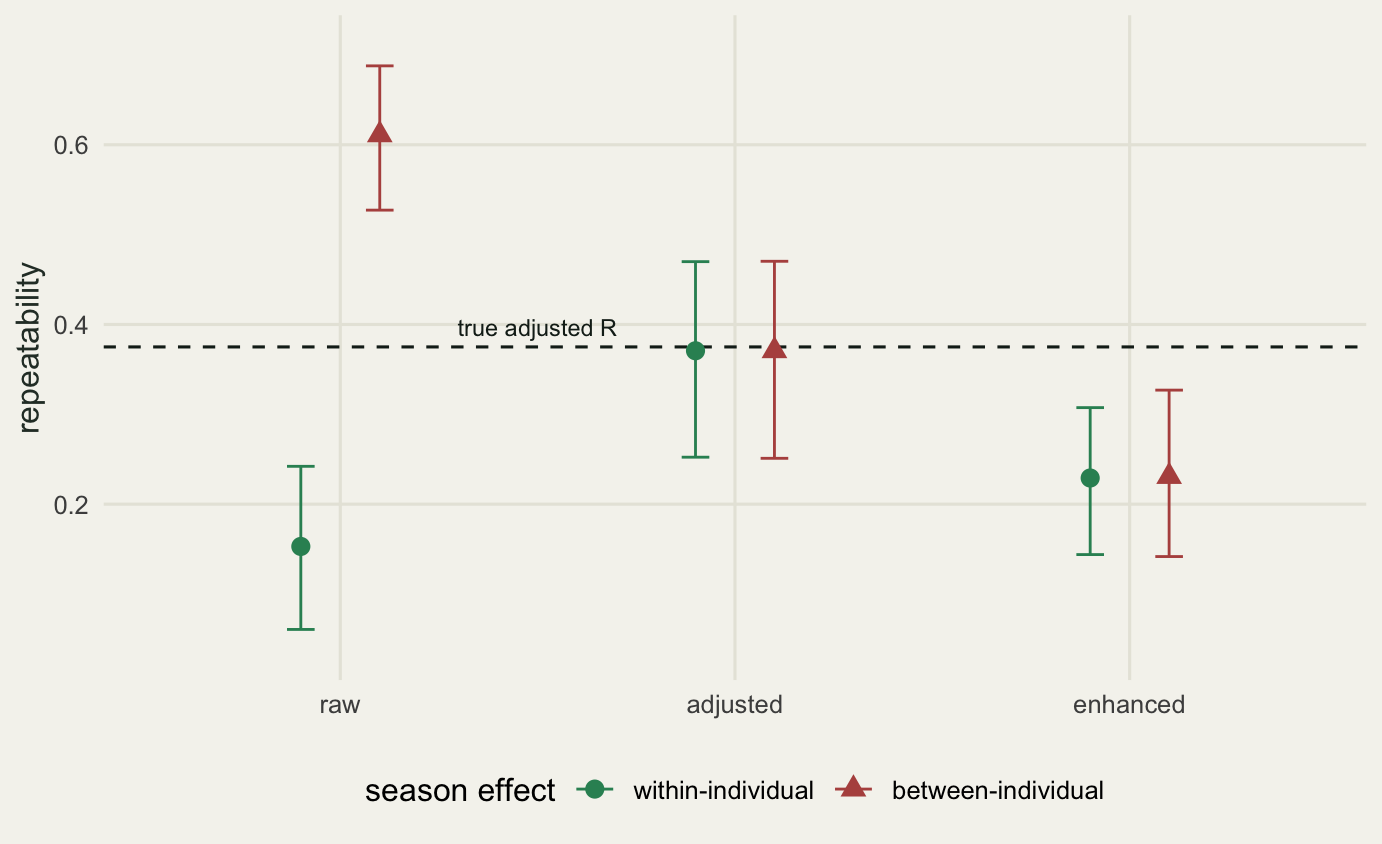
Averaged over 300 replicates the raw repeatability is 0.1530 in the within-individual design and 0.6110 in the between-individual design, a factor of 3.99483. The adjusted repeatability is 0.3707 and 0.3708: the two designs differ by 0.00004. The enhanced version is 0.2291 and 0.2308, differing by 0.00169.
That is not the result the usual framing leads you to expect. The story is normally told as “adjusting raises R when the fixed effect is within individuals and lowers it when the fixed effect is between individuals”, which sounds as though the adjustment has a mind of its own and pushes the answer in a design-dependent direction. The measurement says something else. The adjusted values from the two designs agree to within 0.00004, and the enhanced values agree to within 0.00169. The quantity that moves, by a factor of 3.99483, is the raw one. Both ratios from the previous section are real, but they are ratios to a moving reference, not evidence that the adjustment is unstable.
That reframes what the three numbers are for. The adjusted repeatability estimates a property of the birds, and it came back the same whatever the field schedule did with the seasons. The raw repeatability estimates a property of the birds plus the schedule, and it is only interpretable if you know the schedule. The enhanced version is the raw question answered with the good numerator: it was also design-invariant here, at 0.2291 against 0.2308, because the season contributed the same total variance under both allocations by construction. Change the season slope in one design and that agreement would go, which is the point: the enhanced value is a statement about this population under this sampling regime, and it says so honestly by carrying the fixed-effect variance in its denominator.
The oddity from the previous section resolves in the component columns. In the within-individual design the mean unadjusted among-individual variance is 0.4009 while the adjusted one is 0.5995, so the deflation was not a fluke of one data set. The mechanism is arithmetic. The unadjusted residual variance in that design averages 2.1926, inflated by the ignored season step, and the among-individual variance is recovered by subtracting a share of that residual from the among-individual mean square. Inflate the residual and you over-subtract. The bird means really are untouched by a within-bird season effect, as the argument above said; what is not untouched is the quantity that gets subtracted from them.
Ignoring a within-individual fixed effect therefore damages both halves of the raw ratio: it pads the denominator and it eats the numerator. That is why the raw value falls as far as 0.1530 against a true 0.3750, which is a larger drop than the inflated residual alone would produce. In the between-individual design the same table shows the opposite: unadjusted among-individual variance 1.5953 against adjusted 0.5999, with the residual essentially untouched at 1.0012 and 1.0012. The season effect there is a difference between birds and the unadjusted model has only one place to put it.
Does adjusting eat real individual variance?
There is a standing worry about between-individual fixed effects: if each bird sits in one level of the factor, the factor and the birds are partly confounded, so fitting the factor might soak up genuine individual differences and drag the adjusted repeatability down for no good reason. The worry gets sharper as the factor gets more levels, because with sixty birds and thirty sampling periods there are only two birds per period.
That is testable. Simulate with no fixed effect at all: birds and residuals only, so the true adjusted repeatability is exactly the true raw one, and any gap between them is the cost of the adjustment rather than a difference in what is being estimated. Then fit a between-individual factor with two, ten or thirty levels anyway, and see what it costs.
set.seed(20260731)
lev_set <- c(2, 10, 30); nsim2 <- 200
res <- matrix(NA_real_, length(lev_set), 6)
for (j in seq_along(lev_set)) {
  L   <- lev_set[j]
  lev <- rep(seq_len(L), each = nind / L)
  Xf  <- (outer(lev, seq_len(L), "==") * 1)[idv, , drop = FALSE]
  acc <- matrix(NA_real_, nsim2, 2)
  for (i in seq_len(nsim2)) {
    aa <- rnorm(nind, 0, sqrt(s2a_t))
    ee <- rnorm(nind * nrep, 0, sqrt(s2e_t))
    yv <- aa[idv] + ee
    f0 <- reml_fit(yv, matrix(1, length(yv), 1), idv)
    f1 <- reml_fit(yv, Xf, idv)
    acc[i, ] <- c(f0$among / (f0$among + f0$within),
                  f1$among / (f1$among + f1$within))
  }
  dd <- acc[, 2] - acc[, 1]
  res[j, ] <- c(colMeans(acc), sd(acc[, 1]), sd(acc[, 2]),
                mean(dd), sd(dd) / sqrt(nsim2))
}
dimnames(res) <- list(paste0("levels_", lev_set),
                      c("mean_raw", "mean_adjusted", "sd_raw", "sd_adjusted",
                        "mean_paired_diff", "se_paired_diff"))
print(round(res, 4))
mean_raw mean_adjusted sd_raw sd_adjusted mean_paired_diff
levels_2 0.3672 0.3665 0.0596 0.0610 -0.0007
levels_10 0.3752 0.3754 0.0610 0.0656 0.0002
levels_30 0.3749 0.3651 0.0614 0.0753 -0.0098
se_paired_diff
levels_2 0.0006
levels_10 0.0016
levels_30 0.0039print(round(c(n_replicates = nsim2, n_individuals = nind,
n_levels_low = min(lev_set), n_levels_high = max(lev_set),
birds_per_level_max = nind / min(lev_set),
birds_per_level_min = nind / max(lev_set),
true_R = s2a_t / (s2a_t + s2e_t),
sd_inflation_high = res[3, 4] / res[3, 3]), 4)) n_replicates n_individuals n_levels_low n_levels_high
200.000 60.000 2.000 30.000
birds_per_level_max birds_per_level_min true_R sd_inflation_high
30.000 2.000 0.375 1.227 The worry is mostly wrong, and the part of it that survives is not the part people state. With the low setting, meaning 30 birds per level, the adjusted mean is 0.3665 against a raw mean of 0.3672; the paired difference on the same data sets is -0.0007 with a standard error of 0.0006. With the high setting, meaning 2 birds per level and 30 fixed parameters fitted to 60 birds, the adjusted mean is 0.3651 against 0.3749 raw, a paired difference of -0.0098 with a standard error of 0.0039.
So there is a small downward pull at the high setting, but it is around a tenth of the estimator’s own standard deviation and it would be invisible in any single study. The reason it stays small is the R in REML. The restricted likelihood is built on contrasts that are orthogonal to the fixed part, so the degrees of freedom spent on the factor are accounted for rather than silently charged to the variance components. Plain maximum likelihood, which does not do this, would show a good part of the shrinkage that the worry predicts, and this is the concrete reason the earlier section insisted on the restricted version.
What the extra fixed effects do cost is precision. The standard deviation of the adjusted estimate goes from 0.0610 at the low setting to 0.0753 at the high one, while the raw estimate goes from 0.0596 to 0.0614. That is an inflation of 1.2270 on the same data. Fitting a between-individual factor with many levels is barely a way of biasing R downwards; it is mostly a way of throwing away information about the comparison you care about, because after the factor is fitted the only birds still being compared with each other are birds that shared a level.
The distinction matters, because the two problems have different fixes. Bias would need a different estimator or a correction term. Imprecision needs more birds, or fewer levels, or a level structure that lets birds be compared across it. It also tells you what to do when a reviewer asks for site or year as a fixed effect on a design where every animal sits in one site: agreeing costs you a wider interval far more than it shifts the point estimate, and the wider interval is the honest one.
The honest version of the warning is therefore about the estimand, not the estimator. When the between-individual factor really does explain individual differences, the adjusted repeatability is genuinely lower than the raw one, as the previous section measured. That is not an artefact: it is the correct answer to a different question. The mistake is to fit a factor that stands in for something individual, such as a bird’s territory or its permanent capture site, and then present the adjusted value as though it described how different the birds are, when it describes how different they are once you have already removed the thing that made them different.
Two intervals for R
A repeatability without an interval is not worth much, and R is a ratio of estimated variances, so its sampling distribution is skewed, bounded at both ends, and piles up at zero whenever the among-individual mean square drops below the within-individual one. None of that is friendly to a standard error plus or minus twice itself, which is one reason repeatabilities are so often reported without any interval at all.
Two intervals are in common use. The closed-form interval exploits the fact that, on balanced Gaussian data, the ratio of the two mean squares follows a scaled F distribution, which inverts to an exact interval for R. The parametric bootstrap treats the fitted variance components as if they were the truth, simulates new data sets from them, refits, and takes the middle 95 per cent of the resulting values.
r_moment <- function(Ymat, idx, k, n) {
  gm  <- rowsum(Ymat, idx) / n
  ssw <- colSums((Ymat - gm[idx, , drop = FALSE])^2)
  ssa <- n * colSums(sweep(gm, 2, colMeans(gm))^2)
  msa <- ssa / (k - 1); msw <- ssw / (k * (n - 1))
  list(R = pmax((msa - msw) / (msa + (n - 1) * msw), 0),
       among = pmax((msa - msw) / n, 0), within = msw, msa = msa, msw = msw)
}

anova_ci <- function(msa, msw, k, n, alpha = 0.05) {
  f0 <- msa / msw
  lo <- f0 / qf(1 - alpha / 2, k - 1, k * (n - 1)) - 1
  hi <- f0 / qf(alpha / 2, k - 1, k * (n - 1)) - 1
  c(max(lo / (lo + n), 0), min(hi / (hi + n), 1))
}

boot_r <- function(among, within, k, n, B) {
  idx <- rep(seq_len(k), each = n)
  Y <- matrix(rnorm(k * n * B, 0, sqrt(within)), k * n, B) +
       matrix(rnorm(k * B, 0, sqrt(among)), k, B)[idx, , drop = FALSE]
  r_moment(Y, idx, k, n)$R
}

Rtrue <- s2a_t / (s2a_t + s2e_t)
kk <- 25; nn <- 5; nboot <- 999
set.seed(20260802)
idx1 <- rep(seq_len(kk), each = nn)
y1   <- matrix(rnorm(kk * nn, 0, sqrt(s2e_t)), kk * nn, 1) +
        rnorm(kk, 0, sqrt(s2a_t))[idx1]
m1   <- r_moment(y1, idx1, kk, nn)
ci_a <- anova_ci(m1$msa, m1$msw, kk, nn)
bs   <- boot_r(m1$among, m1$within, kk, nn, nboot)
ci_b <- as.vector(quantile(bs, c(0.025, 0.975)))

print(round(c(n_individuals = kk, n_per_individual = nn,
              n_bootstrap = nboot, R_hat = m1$R, R_true = Rtrue,
              among_hat = m1$among, within_hat = m1$within,
              closed_lo = ci_a[1], closed_hi = ci_a[2],
              boot_lo = ci_b[1], boot_hi = ci_b[2],
              closed_width = ci_a[2] - ci_a[1],
              boot_width = ci_b[2] - ci_b[1],
              boot_mean = mean(bs), boot_median = median(bs)), 4))
n_individuals n_per_individual n_bootstrap R_hat
25.0000 5.0000 999.0000 0.3570
R_true among_hat within_hat closed_lo
0.3750 0.6196 1.1161 0.1826
closed_hi boot_lo boot_hi closed_width
0.5706 0.1388 0.5318 0.3880
boot_width boot_mean boot_median
0.3930 0.3509 0.3545 ggplot(data.frame(R = bs), aes(R)) +
geom_histogram(bins = 40, fill = te_pal$sage, colour = te_pal$paper,
linewidth = 0.2) +
annotate("segment", x = ci_a[1], xend = ci_a[2], y = -6, yend = -6,
colour = te_pal$forest, linewidth = 1.1) +
annotate("point", x = c(ci_a[1], ci_a[2]), y = c(-6, -6),
colour = te_pal$forest, size = 2) +
annotate("text", x = ci_a[2], y = -6, label = "closed form", hjust = -0.08,
size = 3.2, colour = te_pal$forest) +
annotate("segment", x = ci_b[1], xend = ci_b[2], y = -17, yend = -17,
colour = te_pal$clay, linewidth = 1.1) +
annotate("point", x = c(ci_b[1], ci_b[2]), y = c(-17, -17),
colour = te_pal$clay, size = 2) +
annotate("text", x = ci_b[2], y = -17, label = "bootstrap", hjust = -0.08,
size = 3.2, colour = te_pal$clay) +
annotate("segment", x = Rtrue, xend = Rtrue, y = 0, yend = Inf,
linetype = 2, colour = te_pal$ink) +
annotate("text", x = Rtrue, y = Inf, label = "true R", vjust = 1.6,
hjust = -0.15, size = 3.2, colour = te_pal$ink) +
scale_x_continuous(expand = expansion(mult = c(0.03, 0.16))) +
scale_y_continuous(breaks = c(0, 20, 40, 60)) +
labs(x = "bootstrap replicate of R", y = "count") +
theme_te() +
theme(plot.margin = margin(6, 14, 6, 6))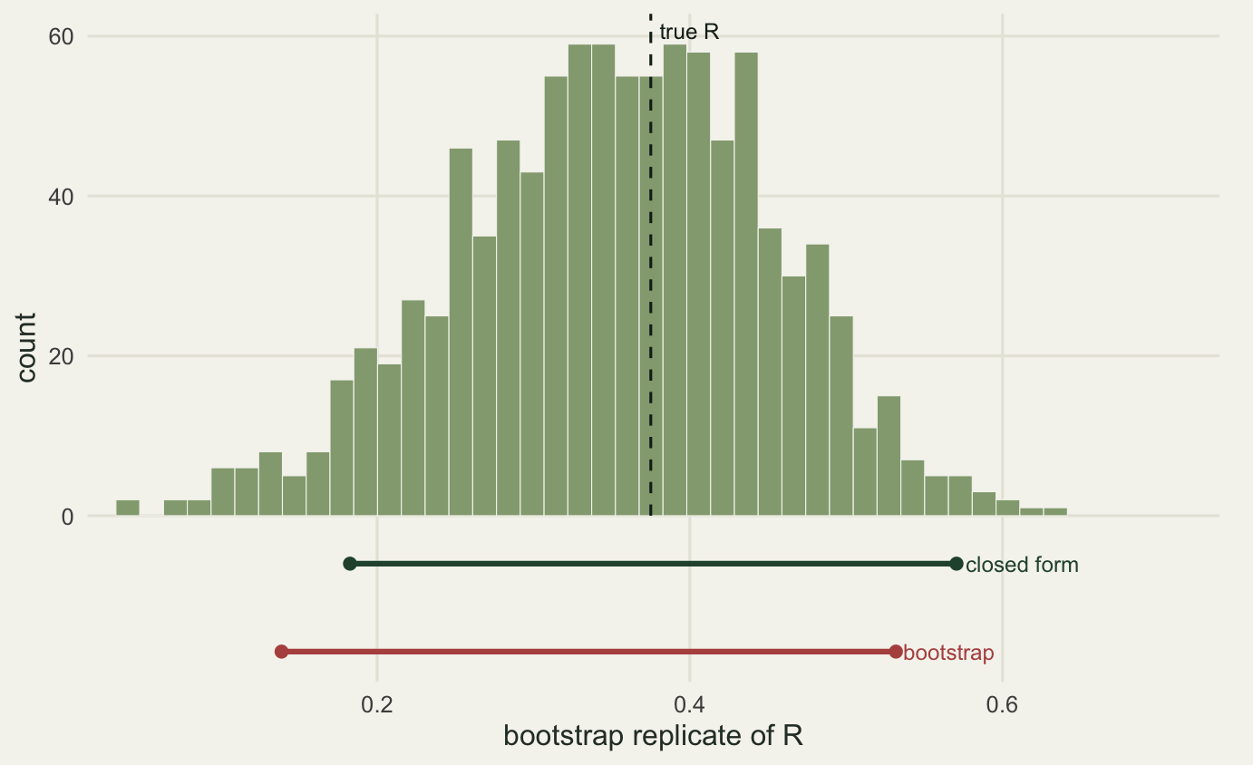
On this data set the point estimate is 0.3570 against a true 0.3750. The closed-form interval runs from 0.1826 to 0.5706 and the bootstrap interval from 0.1388 to 0.5318. Their widths are 0.3880 and 0.3930, close enough to each other, but the bootstrap interval is displaced towards zero at both ends.
The displacement is structural rather than accidental. The bootstrap simulates from 0.6196 and 1.1161, the estimated components, so the cloud of replicate values is centred near the estimate: the bootstrap mean is 0.3509 and the median 0.3545, both close to the 0.3570 it started from. A percentile interval then puts its two endpoints where those replicates fall. When the estimate happens to be low, as here, the whole interval follows it down instead of reaching up to cover the values that could plausibly have produced a low estimate. The closed-form interval does not have this problem, because it inverts a pivotal quantity whose distribution does not depend on where the estimate landed.
Both intervals here are wide. Twenty-five individuals measured five times each gives an interval about 0.3880 wide on a scale that only runs from zero to one, so that same fraction of the whole range stays compatible with the data. Published repeatabilities from small studies are frequently given to three decimal places with an interval half the unit interval wide, and the decimals are decoration.
What the intervals actually cover
An interval that looks reasonable is not the same as an interval that covers. Run six hundred fresh data sets at each of three designs, build both intervals on every one, and count how often the true R falls inside. Six hundred replicates puts a standard error of about nine parts in a thousand on each coverage figure, which is fine enough to see a shortfall of a few percentage points and not fine enough to argue about one. The bootstrap uses fewer resamples per data set here than in the single-data-set example above, which is what keeps the whole study inside a few seconds; that costs a little resolution in the percentile endpoints and none of the conclusion.
set.seed(20260803)
n_set <- c(3, 5, 10); nsim3 <- 600; nboot_c <- 199
cov_tab <- matrix(NA_real_, length(n_set), 6)
for (j in seq_along(n_set)) {
  n <- n_set[j]; idx <- rep(seq_len(kk), each = n)
  hit_a <- 0; hit_b <- 0; low_a <- 0; low_b <- 0
  wid_a <- numeric(nsim3); wid_b <- numeric(nsim3)
  for (i in seq_len(nsim3)) {
    yv <- matrix(rnorm(kk * n, 0, sqrt(s2e_t)), kk * n, 1) +
          rnorm(kk, 0, sqrt(s2a_t))[idx]
    mm <- r_moment(yv, idx, kk, n)
    ca <- anova_ci(mm$msa, mm$msw, kk, n)
    cb <- as.vector(quantile(boot_r(mm$among, mm$within, kk, n, nboot_c),
                             c(0.025, 0.975)))
    hit_a <- hit_a + (ca[1] <= Rtrue && Rtrue <= ca[2])
    hit_b <- hit_b + (cb[1] <= Rtrue && Rtrue <= cb[2])
    low_a <- low_a + (ca[2] < Rtrue)
    low_b <- low_b + (cb[2] < Rtrue)
    wid_a[i] <- ca[2] - ca[1]; wid_b[i] <- cb[2] - cb[1]
  }
  cov_tab[j, ] <- c(hit_a / nsim3, hit_b / nsim3, mean(wid_a), mean(wid_b),
                    low_a / nsim3, low_b / nsim3)
}
dimnames(cov_tab) <- list(paste0("n_", n_set),
                          c("cover_closed", "cover_boot", "width_closed",
                            "width_boot", "miss_low_closed", "miss_low_boot"))
print(round(cov_tab, 4))
cover_closed cover_boot width_closed width_boot miss_low_closed
n_3 0.9533 0.9183 0.4682 0.4577 0.0217
n_5 0.9467 0.9317 0.3789 0.3697 0.0217
n_10 0.9383 0.9200 0.3167 0.3030 0.0300
miss_low_boot
n_3 0.0600
n_5 0.0550
n_10 0.0667print(round(c(n_replicates = nsim3, n_bootstrap = nboot_c,
n_individuals = kk, nominal = 0.95, nominal_percent = 95,
noncoverage_budget = 0.05,
mc_se = sqrt(0.95 * 0.05 / nsim3),
mean_cover_closed = mean(cov_tab[, 1]),
mean_cover_boot = mean(cov_tab[, 2]),
shortfall_boot = 0.95 - mean(cov_tab[, 2])), 4)) n_replicates n_bootstrap n_individuals nominal
600.0000 199.0000 25.0000 0.9500
nominal_percent noncoverage_budget mc_se mean_cover_closed
95.0000 0.0500 0.0089 0.9461
mean_cover_boot shortfall_boot
0.9233 0.0267 gcov <- data.frame(n = rep(n_set, 2),
cov = c(cov_tab[, 1], cov_tab[, 2]),
method = factor(rep(c("closed form", "parametric bootstrap"),
each = length(n_set))))
gcov$se <- sqrt(gcov$cov * (1 - gcov$cov) / nsim3)
ggplot(gcov, aes(n, cov, colour = method, shape = method)) +
geom_hline(yintercept = 0.95, linetype = 2, colour = te_pal$ink) +
geom_line(aes(group = method), linewidth = 0.5,
position = position_dodge(width = 0.35)) +
geom_errorbar(aes(ymin = cov - 2 * se, ymax = cov + 2 * se), width = 0.25,
linewidth = 0.5, position = position_dodge(width = 0.35)) +
geom_point(size = 3, position = position_dodge(width = 0.35)) +
scale_colour_manual(values = c(te_pal$forest, te_pal$clay)) +
scale_shape_manual(values = c(16, 17)) +
scale_x_continuous(breaks = n_set, expand = expansion(mult = 0.1)) +
scale_y_continuous(expand = expansion(mult = 0.1)) +
labs(x = "measurements per individual",
y = "coverage of the interval", colour = NULL, shape = NULL) +
theme_te()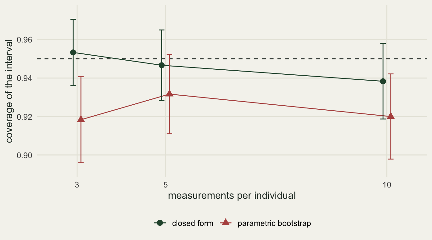
The closed-form interval covers. Its three figures are 0.9533, 0.9467 and 0.9383 against a nominal 0.95, with a Monte Carlo standard error of 0.0089 on each, so all three sit within about two standard errors of where they should be. Their mean is 0.9461. That is the expected result on balanced Gaussian data generated from exactly the model the interval assumes, and it is the benchmark the bootstrap has to beat.
It does not. The bootstrap covers 0.9183, 0.9317 and 0.9200, mean 0.9233, a shortfall of 0.0267 that is several standard errors from nominal in the pooled comparison and shows no sign of closing as the number of repeats rises. Part of it is width: the bootstrap intervals average 0.4577, 0.3697 and 0.3030 against 0.4682, 0.3789 and 0.3167 for the closed form, so they are slightly shorter everywhere.
Most of it is position, and the miss columns show it. Counting only the misses where the whole interval lies below the truth, the bootstrap fails that way on 0.0600, 0.0550 and 0.0667 of data sets, against 0.0217, 0.0217 and 0.0300 for the closed form. The closed form spreads its errors roughly evenly between the two sides, as a well-behaved interval should. The bootstrap does not: a low-side miss rate of 0.0667 out of a total non-coverage budget of 0.05 means it throws most of its errors in one direction. It sits too low, exactly as the single data set in the previous section suggested it would.
The practical consequence is specific rather than general. A percentile bootstrap interval for a repeatability will tend to understate how high R could be, so a study that reports one and concludes the trait is only weakly repeatable has slightly more of a case to answer than its interval suggests. The effect is small on this scale. It is not small enough to ignore when the whole argument of a paper rests on whether an interval excluded some value.
None of this makes the parametric bootstrap useless. It is the only one of the two that survives unbalanced data, non-Gaussian responses or extra random effects, where no closed form exists, and the standard tooling for repeatability in R leans on it for that reason. The measurement here says something narrower: on the one design where an exact interval exists, the percentile bootstrap is worse, and the way it is worse is a systematic tilt rather than random noise. If you are running the bootstrap on a design where the closed form applies, use the closed form. If you are running it elsewhere, expect the interval to be a little short and a little low, and do not read its endpoints as though they were exact.
What to take away
Compute the adjusted repeatability and say that is what you computed. It is the one that estimates a property of the animals rather than a property of the animals combined with the field schedule, and in the simulation it returned 0.3707 and 0.3708 from two designs that put the season effect in completely different places. The raw value moved by a factor of 3.99483 between those same two designs. If you report a raw repeatability, report it alongside the design, because on its own it does not mean anything a reader can use. If you report the enhanced version, say which fixed effects went into its denominator, because that is what defines it.
The direction the adjustment moves the number is not a property of adjusting. It follows from where the fixed effect sits relative to individual identity, and both directions happen: 2.7828 times the raw value when the effect varies within individuals, 0.6376 times it when the effect varies between them. There is no rule of thumb here to memorise. Look at how the covariate is distributed across individuals, and the direction follows from that alone.
Here is the honest limit, and it is a large one. A repeatability is not a constant of a species or a trait. It depends on which population you sampled, because R falls when the individuals happen to be alike; on how long you left between measurements, because within-individual variance grows with the gap and R falls with it; and on which fixed effects the analyst decided to fit, because that choice is precisely what separates the numerator from the denominator. Every number in this post came from data whose true variance components were known and fixed, and even under those conditions the raw definition alone ran from 0.1530 to 0.6110 across the two allocations of the season effect. In real data none of those conditions hold. A repeatability is only interpretable next to a description of the design that produced it, and comparing two published values without that description is not a comparison of anything.
References
Biro PA, Stamps JA 2015 Animal Behaviour 105:223-230 (10.1016/j.anbehav.2015.04.008)
Dingemanse NJ, Dochtermann NA 2013 Journal of Animal Ecology 82(1):39-54 (10.1111/1365-2656.12013)
Donner A, Wells G 1986 Biometrics 42(2):401-412 (10.2307/2531060)
Lessells CM, Boag PT 1987 The Auk 104(1):116-121 (10.2307/4087240)
Nakagawa S, Schielzeth H 2010 Biological Reviews 85(4):935-956 (10.1111/j.1469-185X.2010.00141.x)
Stoffel MA, Nakagawa S, Schielzeth H 2017 Methods in Ecology and Evolution 8(11):1639-1644 (10.1111/2041-210X.12797)
Wolak ME, Fairbairn DJ, Paulsen YR 2012 Methods in Ecology and Evolution 3(1):129-137 (10.1111/j.2041-210X.2011.00125.x)