library(ggplot2)

te_paper  <- "#f5f4ee"
te_ink    <- "#16241d"
te_body   <- "#2c3a31"
te_forest <- "#275139"
te_rust   <- "#b5534e"
te_line   <- "#dad9ca"

theme_datasheet <- function() {
  theme_minimal(base_size = 12) +
    theme(plot.background  = element_rect(fill = te_paper, colour = NA),
          panel.background = element_rect(fill = te_paper, colour = NA),
          panel.grid.major = element_line(colour = te_line, linewidth = 0.3),
          panel.grid.minor = element_blank(),
          text             = element_text(colour = te_body),
          plot.title       = element_text(colour = te_ink, face = "bold"),
          axis.text        = element_text(colour = te_body))
}

# observed agreement, chance agreement and kappa from a square confusion matrix
kappa_hand <- function(m) {
  n  <- sum(m)
  po <- sum(diag(m)) / n
  pe <- sum(rowSums(m) * colSums(m)) / n^2
  c(agreement = po, expected = pe, kappa = (po - pe) / (1 - pe))
}Observer agreement and Cohen’s kappa in R
R
measurement error
survey design
statistics
ecology tutorial
Per cent agreement flatters two surveyors, and Cohen’s kappa moves with class prevalence. Simulate both in base R and weight kappa for ordered cover classes.
Corrected 1 October 2026: the post said the rise in per cent agreement as mire gets rarer is mild because the surveyors are accurate, and steeper if they were less so; it now says the rise comes from the gap between the accuracies on the two classes, and that with equal accuracies there would be none.
Corrected 30 September 2026: the post said PABAK fixes the prevalence dependence; it now says PABAK removes the marginals from the formula but still moves with prevalence through per cent agreement.
Two surveyors walk the same 200 quadrats and each writes down a habitat class. Back in the office someone counts the quadrats where the cards match, divides by 200, and reports a percentage. If the site is a mosaic of mire and grassland in roughly equal parts, that number means something. If the site is grassland with a few wet flushes in it, a surveyor who wrote “grassland” on every card without looking up would still match a careful colleague on nearly every quadrat, and the count would be measuring the site, not the surveyors.
Cohen’s kappa exists to fix exactly that. It subtracts the agreement two observers would reach by chance alone, given how often each of them uses each class, and rescales what is left. The instinct is right. What is less often said is that the correction imports the prevalence of the classes into the answer: two surveyors whose per-class accuracy never changes will produce a different kappa on a different site. Over the sweep below it runs from about an eighth to about three quarters, the distance from “slight” to “substantial” on the usual benchmark table.
Everything here apart from the plots is base R. The arithmetic is fifteen lines, worth having in your fingers because the number it produces is one you will have to defend.
Agreement, chance, and kappa by hand
pe is the whole idea. Multiply the row total for a class by the column total for the same class, sum over classes, divide by the square of the sample size: that is the agreement two observers would reach if each kept their own habit of using the classes but assigned quadrats at random.
Now a generator where the truth is known. Each quadrat has a true class; each surveyor gets it right with a probability that depends on that class, and errs independently of the other.
classify <- function(truth, acc) {
  ok <- runif(length(truth)) < acc[truth]
  ifelse(ok, truth, 3L - truth)
}

survey <- function(n, prev_rare, acc) {
  truth <- sample(1:2, n, replace = TRUE, prob = c(prev_rare, 1 - prev_rare))
  lab   <- c("mire", "grassland")
  table(surveyor_A = factor(lab[classify(truth, acc)], lab),
        surveyor_B = factor(lab[classify(truth, acc)], lab))
}

acc <- c(mire = 0.90, grassland = 0.95)
set.seed(1)
balanced <- survey(200, 0.5, acc)
balanced
surveyor_B
surveyor_A mire grassland
mire 84 11
grassland 17 88round(kappa_hand(balanced), 3)agreement expected kappa
0.86 0.50 0.72 round(c(agreement_expected = sum(0.5 * (acc^2 + (1 - acc)^2))), 4)agreement_expected
0.8625 Two surveyors who are 90 and 95 per cent accurate on the two classes agreed on 86.0 per cent of the quadrats, against an expectation of 86.25 per cent from the known truth, and kappa came out at 0.72. Seed 1 is used because it gives a middling draw rather than a flattering one; the last section shows how far kappa scatters between surveys of this size, at a lower mire prevalence. The reflex is to load irr or psych; a package returns the same 0.72 without showing what pe is made of, and pe is the part a referee will ask about.
The same two surveyors, a different kappa
Hold the accuracy fixed. Nobody retrains, nobody buys a better field guide. Only the site changes: mire goes from half the quadrats to one in a hundred. The sweep uses very large surveys to keep sampling noise out of the picture, so what moves is the estimand and not the estimate.
prev_grid <- exp(seq(log(0.5), log(0.01), length.out = 30))
set.seed(11)
sweep_out <- data.frame(prevalence = prev_grid,
                        agreement = NA_real_, kappa = NA_real_)
for (i in seq_along(prev_grid)) {
  k <- kappa_hand(survey(60000, prev_grid[i], acc))
  sweep_out$agreement[i] <- k[["agreement"]]
  sweep_out$kappa[i]     <- k[["kappa"]]
}
round(sweep_out[c(1, 10, 20, 30), ], 4)
prevalence agreement kappa
1 0.5000 0.8622 0.7239
10 0.1485 0.8898 0.6195
20 0.0385 0.9012 0.3545
30 0.0100 0.9047 0.1259round(c(kappa_low = min(sweep_out$kappa), kappa_high = max(sweep_out$kappa),
agreement_low = min(sweep_out$agreement),
agreement_high = max(sweep_out$agreement)), 4) kappa_low kappa_high agreement_low agreement_high
0.1259 0.7245 0.8622 0.9047 Per cent agreement went up, from 86.2 to 90.5 per cent, as the site got more lopsided. That is the failure the opening paragraph described, mild here because the two classes are identified almost equally well: the climb comes from the gap between the two per-class accuracies, and with equal accuracies there would be none. Kappa went the other way, from 0.724 at an even split to 0.126 at one mire quadrat in a hundred, a factor of about six.
It is not quite monotone either, and reading the wobble off the sweep would be reading noise: the largest kappa on the grid sits 0.0006 above the value at the even split, and every point is a single draw. For two classes the population kappa is four lines of the same quantities, with no simulation in it.
# population kappa from prevalence and the two per-class accuracies
kappa_pop <- function(p, se = acc[["mire"]], sp = acc[["grassland"]]) {
  q  <- p * se + (1 - p) * (1 - sp)   # chance either surveyor writes "mire"
  po <- p * (se^2 + (1 - se)^2) + (1 - p) * (sp^2 + (1 - sp)^2)
  pe <- q^2 + (1 - q)^2
  (po - pe) / (1 - pe)
}
peak <- optimize(kappa_pop, c(0.01, 0.99), maximum = TRUE)
round(c(peak_prevalence = peak$maximum, peak_kappa = peak$objective,
        even_split = kappa_pop(0.5), one_in_a_hundred = kappa_pop(0.01)), 3)
peak_prevalence peak_kappa even_split one_in_a_hundred
0.421 0.729 0.724 0.130 The bump is real and interior, but not where the sweep put it: kappa peaks near a prevalence of 0.42, at 0.729 against 0.724 at the even split, then falls away either side. A bump of 0.005 is small; the collapse below a prevalence of about 0.2 is not, and both ends describe the same surveyors making the same mistakes at the same rates.
long <- data.frame(
  prevalence = rep(sweep_out$prevalence, 2),
  value      = c(sweep_out$agreement, sweep_out$kappa),
  measure    = rep(c("per cent agreement", "Cohen's kappa"),
                   each = nrow(sweep_out)))

ggplot(long, aes(x = prevalence, y = value, colour = measure)) +
  geom_hline(yintercept = c(0.2, 0.4, 0.6), linetype = "dotted",
             colour = te_body, linewidth = 0.3) +
  geom_line(linewidth = 1) +
  scale_x_log10(breaks = c(0.01, 0.02, 0.05, 0.1, 0.2, 0.5)) +
  scale_colour_manual(values = c(te_rust, te_forest)) +
  ylim(0, 1) +
  labs(x = "prevalence of the rarer class", y = NULL, colour = NULL,
       title = "Same surveyors, same accuracy, a moving kappa") +
  theme_datasheet() +
  theme(legend.position = "bottom")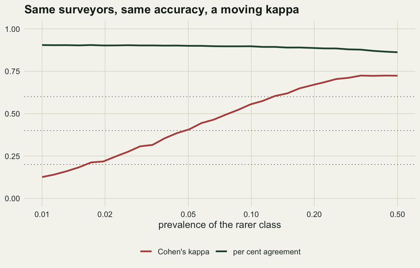
A kappa copied out of one paper therefore cannot be compared with a kappa in another: the two were computed on sites with different class mixtures, and the benchmark tables that turn a kappa into a word are silent about that. Surveyors called “substantial” on a mixed site are “fair” where the interesting habitat is scarce.
What else moves kappa at a fixed level of agreement
Prevalence is not the only thing loose in the denominator. Fix the per cent agreement at 0.85 in a 200-quadrat survey and ask what kappa is still free to do.
grid_po <- expand.grid(a = 0:170, b = 0:30)
grid_po$kappa <- mapply(function(a, b)
  kappa_hand(matrix(c(a, 30 - b, b, 170 - a), 2, 2))[["kappa"]],
  grid_po$a, grid_po$b)
round(range(grid_po$kappa[is.finite(grid_po$kappa)]), 3)
[1] -0.081 0.707Every one of those tables has 170 matching quadrats out of 200. Kappa runs from -0.081 to 0.707, so per cent agreement pins kappa down hardly at all.
The second thing moving inside that range is the difference between the two observers’ marginal totals, and here kappa behaves in a way most readers do not expect. Take two tables with identical agreement. In the first the disagreements are symmetric, fifteen quadrats each way. In the second they are entirely one-sided: B calls thirty quadrats mire that A calls grassland, and never the reverse.
same_po <- list(
  symmetric = matrix(c(45, 15,  15, 125), 2, 2, byrow = TRUE),
  one_sided = matrix(c(45,  0,  30, 125), 2, 2, byrow = TRUE))

round(t(sapply(same_po, function(m)
  c(kappa_hand(m), pabak = 2 * sum(diag(m)) / sum(m) - 1))), 3)
agreement expected kappa pabak
symmetric 0.85 0.580 0.643 0.7
one_sided 0.85 0.569 0.652 0.7sapply(same_po, function(m)
formatC(mcnemar.test(m)$p.value, format = "e", digits = 1))symmetric one_sided
"1.0e+00" "1.2e-07" The second table is a surveyor with a systematic habit, serious and fixable: B’s mire is not A’s mire, and any area estimate from B’s cards will be too high. Per cent agreement is 0.85 in both. Kappa is 0.643 and 0.652, very slightly higher where the bias is, which is Feinstein and Cicchetti’s second paradox: disagreeing about how often to use a class lowers the chance agreement and props kappa up. Neither summary flags the thing that matters. The marginals do, and a McNemar test on the off-diagonal cells separates the two tables at once.
Prevalence-adjusted bias-adjusted kappa is one published response to the first paradox, replacing the observed marginals with even ones, which collapses to 2 * po - 1: for both tables above, 0.70. That takes the marginals out of the formula but not all of the prevalence dependence, because per cent agreement itself moved with prevalence in the sweep above and PABAK is a rescaling of it. It also makes PABAK per cent agreement on a stretched scale, unable to separate any two tables that agree equally often, including the pair here and the surveyor who wrote grassland on every card. Report it with the per cent agreement and the two marginal distributions beside it, because that is what PABAK threw away.
Ordered classes: adjacent errors should not cost full price
Braun-Blanquet cover classes are ordered, as are DAFOR scales and most rapid habitat assessments. Unweighted kappa treats them as names: calling a class-1 quadrat class 5 costs the same as calling it class 2, which is not how anyone reads a cover chart. Weighted kappa gives partial credit instead, and the weight matrix is one line of outer.
set.seed(20260813)
n_quad   <- 300
true_cov <- sample(1:5, n_quad, replace = TRUE, prob = c(.30, .25, .20, .15, .10))

slip <- function(x) {
  step <- sample(c(0, -1, 1, -2, 2), length(x), replace = TRUE,
                 prob = c(0.60, 0.17, 0.17, 0.03, 0.03))
  pmin(pmax(x + step, 1), 5)
}
cov_A <- slip(true_cov)
cov_B <- slip(true_cov)
cover <- table(surveyor_A = factor(cov_A, 1:5), surveyor_B = factor(cov_B, 1:5))
cover
surveyor_B
surveyor_A 1 2 3 4 5
1 50 24 6 2 0
2 19 30 10 2 0
3 8 20 23 16 7
4 1 2 10 20 7
5 0 0 5 10 28round(kappa_hand(cover), 3)agreement expected kappa
0.503 0.209 0.372 k_classes <- 5
w_lin <- 1 - abs(outer(1:k_classes, 1:k_classes, "-")) / (k_classes - 1)
w_quad <- 1 - (outer(1:k_classes, 1:k_classes, "-") / (k_classes - 1))^2
kappa_weighted <- function(m, w) {
p <- m / sum(m)
pm <- outer(rowSums(p), colSums(p))
(sum(w * p) - sum(w * pm)) / (1 - sum(w * pm))
}
round(c(unweighted = kappa_hand(cover)[["kappa"]],
linear = kappa_weighted(cover, w_lin),
quadratic = kappa_weighted(cover, w_quad)), 3)unweighted linear quadratic
0.372 0.602 0.770 apart <- abs(cov_A - cov_B)
table(classes_apart = apart)classes_apart
0 1 2 3
151 116 30 3 round(mean(apart[apart > 0] == 1), 3)[1] 0.779The two surveyors put the same quadrat in the same class only 50.3 per cent of the time, and unweighted kappa reports 0.37. But 78 per cent of the disagreements are by a single class, and only 3 quadrats out of 300 are more than two apart. Linear weights raise kappa to 0.60 and quadratic weights to 0.77.
cover_df <- as.data.frame(cover)
names(cover_df) <- c("A", "B", "count")

ggplot(cover_df, aes(x = B, y = A, fill = count)) +
  geom_tile(colour = te_paper, linewidth = 1) +
  geom_text(aes(label = count, colour = count > 35), size = 3.4) +
  scale_fill_gradient(low = te_paper, high = te_forest) +
  scale_colour_manual(values = c("FALSE" = te_ink, "TRUE" = te_paper)) +
  labs(x = "surveyor B, cover class", y = "surveyor A, cover class",
       title = "Most disagreement is one class wide") +
  theme_datasheet() +
  theme(panel.grid = element_blank(), legend.position = "none")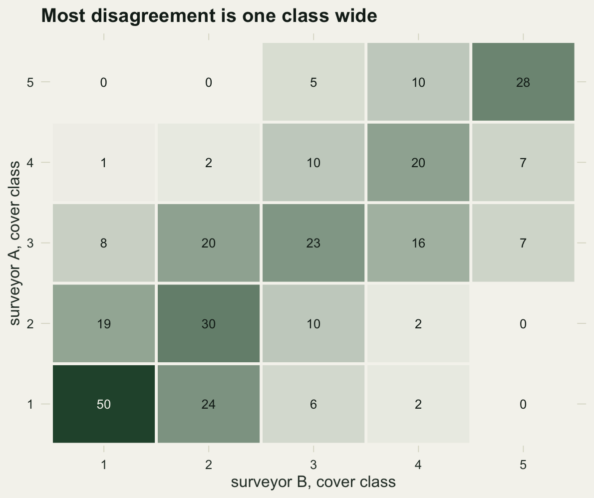
Which weights? Linear says a two-class error is twice as bad as a one-class error, quadratic four times as bad. Quadratic has a property worth knowing: quadratic-weighted kappa is the two-way intraclass correlation for absolute agreement, treating the class numbers as measurements (Fleiss and Cohen 1973). Two-way, not one-way, and what separates the two is marginal bias, the subject of the section before this.
icc_two_way <- function(m) {   # ICC(A,1): subjects in rows, observers in columns
  n <- nrow(m); k <- ncol(m); gm <- mean(m)
  msr <- k * sum((rowMeans(m) - gm)^2) / (n - 1)          # between subjects
  msc <- n * sum((colMeans(m) - gm)^2) / (k - 1)          # between observers
  mse <- (sum((m - gm)^2) - (n - 1) * msr - (k - 1) * msc) / ((n - 1) * (k - 1))
  (msr - mse) / (msr + (k - 1) * mse + k * (msc - mse) / n)
}
icc_one_way <- function(m) {          # written for two raters, as used here
  rm_ <- rowMeans(m); gm <- mean(m)
  msb <- ncol(m) * sum((rm_ - gm)^2) / (nrow(m) - 1)
  msw <- sum((m - rm_)^2) / (nrow(m) * (ncol(m) - 1))
  (msb - msw) / (msb + msw)
}
pair    <- cbind(cov_A, cov_B)
shifted <- cbind(cov_A, pmin(cov_B + 1, 5))   # give B a one-class habit
cover_s <- table(factor(shifted[, 1], 1:5), factor(shifted[, 2], 1:5))
qk      <- c(kappa_weighted(cover, w_quad), kappa_weighted(cover_s, w_quad))
compare <- rbind(quadratic_kappa = qk,
                 icc_two_way = c(icc_two_way(pair), icc_two_way(shifted)),
                 icc_one_way = c(icc_one_way(pair), icc_one_way(shifted)))
colnames(compare) <- c("as_recorded", "B_shifted")
round(compare, 4)
as_recorded B_shifted
quadratic_kappa 0.7698 0.6014
icc_two_way 0.7704 0.6022
icc_one_way 0.7704 0.5618round(c(mean_A = mean(cov_A), mean_B = mean(cov_B)), 3) # matched marginalsmean_A mean_B
2.670 2.673 On the recorded pair, whose mean scores differ by 0.003 of a class, all three agree to within 0.0007 and either version would have passed. Push every one of B’s scores up a class, as far as the top class allows, and they part company: the two-way figure stays within 0.0008 of the weighted kappa, while the one-way figure falls 0.040 below it, having nowhere to put a systematic difference between observers and charging it to error.
The equivalence is also a warning: quadratic weights are a decision that the classes are equally spaced numbers, which Braun-Blanquet cover bands are emphatically not. If you will make that assumption, the intraclass correlation is better documented territory, covered here in Adjusted repeatability in R and Checking a repeatability analysis. If you will not, stay with linear weights and say so.
Six observers instead of two
Cohen’s kappa is defined for a named pair. With a panel scoring the same recordings, Fleiss’s kappa asks a different question: how much do raters drawn from this pool agree, treated as interchangeable. It needs only the counts of raters choosing each category per subject.
set.seed(99)
n_rec <- 120
n_sp  <- 4
sp_truth <- sample(1:n_sp, n_rec, replace = TRUE, prob = c(.4, .3, .2, .1))
skill    <- c(0.90, 0.88, 0.90, 0.86, 0.89, 0.55)
scores   <- sapply(skill, function(a)
  ifelse(runif(n_rec) < a, sp_truth, sample(1:n_sp, n_rec, replace = TRUE)))

correct <- colMeans(scores == sp_truth)
round(correct, 3)
[1] 0.908 0.958 0.933 0.850 0.933 0.767counts <- t(apply(scores, 1, function(r) tabulate(r, n_sp)))
fleiss_kappa <- function(counts) { # constant panel size, as here
raters <- sum(counts[1, ])
subj <- nrow(counts)
p_cat <- colSums(counts) / (subj * raters)
p_subj <- (rowSums(counts^2) - raters) / (raters * (raters - 1))
(mean(p_subj) - sum(p_cat^2)) / (1 - sum(p_cat^2))
}
pairs_ij <- combn(ncol(scores), 2)
pairwise <- apply(pairs_ij, 2, function(p)
kappa_hand(table(factor(scores[, p[1]], 1:n_sp),
factor(scores[, p[2]], 1:n_sp)))[["kappa"]])
round(c(fleiss = fleiss_kappa(counts),
mean_pairwise_cohen = mean(pairwise),
lowest_pair = min(pairwise), highest_pair = max(pairwise)), 3) fleiss mean_pairwise_cohen lowest_pair highest_pair
0.721 0.722 0.583 0.844 round(sapply(seq_len(ncol(scores)), function(k)
mean(pairwise[apply(pairs_ij, 2, function(p) k %in% p)])), 3)[1] 0.739 0.768 0.759 0.698 0.761 0.607Fleiss returns 0.721 and the mean of the fifteen pairwise Cohen kappas is 0.722, which is the sense in which they answer nearly the same question. The pairs run from 0.58 to 0.84, and the last row shows why. Observer six listens to the recording only 55 per cent of the time and guesses otherwise, and a guess still lands on the right category some of the time, so the generator gives them about 66 per cent right in the long run; in this draw they were right on 77 per cent of the recordings, against 92 per cent for the other five, which is enough to put their mean pairwise kappa lowest of the six. No panel-level number tells you that; the per-observer means take one more line, and in a training exercise that line is the point.
Honest limits
The benchmark tables come first: the most quoted thing in this literature and the least defensible. The slight, fair, moderate, substantial and almost perfect bands were offered as a convenience with no theoretical backing, and their authors said so. The sweep should settle it: one unchanged pair of surveyors crossed three of those boundaries because the vegetation map changed under them.
The simulation assumes the two surveyors err independently. Real observers are trained together, carry the same field guide, and misread the same ambiguous flush the same way, and every measure here treats that shared error as agreement. Correlated errors inflate per cent agreement, kappa and the weighted versions alike, and nothing computed from the two cards alone separates shared competence from shared mistake. Hence the occasional specimen-verified quadrat.
Agreement is not accuracy either. Two surveyors who both call every flush “grassland” agree perfectly and are both wrong. Kappa answers whether the classification is reproducible, a precondition for accuracy rather than evidence of it. If you want accuracy you need a truth column, and the quantity to report is a per-class error rate.
Sampling error in kappa is also large at the sizes people actually survey.
set.seed(7)
reps <- replicate(500, kappa_hand(survey(200, 0.10, acc))[["kappa"]])
round(c(mean = mean(reps), sd = sd(reps), quantile(reps, c(0.025, 0.975))), 3)
mean sd 2.5% 97.5%
0.548 0.089 0.368 0.710 Five hundred repeats of a 200-quadrat survey at a mire prevalence of 0.10, with the accuracies held fixed, put kappa’s standard deviation at 0.089 and its central 95 per cent between 0.37 and 0.71. That interval spans three benchmark bands on its own, before anything about the site or surveyors changes. The sweep used 60000 quadrats per point so that this scatter would not obscure the systematic movement; a real survey has no such luxury. Finally, two classes make the prevalence argument visible, but with more classes there are more marginals free to move and the problem is harder to see, not smaller.
References
Byrt T, Bishop J, Carlin JB 1993 Journal of Clinical Epidemiology 46(5):423-429 (10.1016/0895-4356(93)90018-V)
Cohen J 1960 Educational and Psychological Measurement 20(1):37-46 (10.1177/001316446002000104)
Cohen J 1968 Psychological Bulletin 70(4):213-220 (10.1037/h0026256)
Feinstein AR, Cicchetti DV 1990 Journal of Clinical Epidemiology 43(6):543-549 (10.1016/0895-4356(90)90158-L)
Fleiss JL 1971 Psychological Bulletin 76(5):378-382 (10.1037/h0031619)
Fleiss JL, Cohen J 1973 Educational and Psychological Measurement 33(3):613-619 (10.1177/001316447303300309)
Landis JR, Koch GG 1977 Biometrics 33(1):159-174 (10.2307/2529310)