library(ggplot2)

te_pal <- list(forest = "#275139", green = "#2f8f63", sage = "#93a87f",
               clay = "#b5534e", gold = "#cda23f", line = "#dad9ca",
               ink = "#16241d", paper = "#f5f4ee")

fmt <- function(x, digits = 4) formatC(x, format = "f", digits = digits)

theme_te <- function() {
  theme_minimal(base_size = 12) +
    theme(panel.grid.minor = element_blank(),
          panel.grid.major = element_line(colour = "#e7e6dc"),
          plot.background = element_rect(fill = "#f5f4ee", colour = NA),
          panel.background = element_rect(fill = "#f5f4ee", colour = NA),
          plot.title = element_text(face = "bold", colour = te_pal$ink),
          axis.title = element_text(colour = "#2c3a31"),
          legend.position = "bottom")
}Checking a repeatability analysis
R
behaviour
repeatability
model checking
ecology tutorial
Four measured checks on a behavioural repeatability estimate in R: design efficiency, the gap between repeats, observer confounding, and the zero boundary.
The great tit boxes were checked on a Tuesday in March, and every bird that went into a bag came back out with a number: seconds spent motionless after release into a novel room. Those numbers went into a spreadsheet over three weeks, and by April the spreadsheet had turned into a single value sitting in the abstract of a draft. The draft said the trait was moderately repeatable and therefore worth treating as a personality axis.
That value is a ratio of two variance components, and it is doing a lot of work. It decides whether the trait gets called personality, and it sets the ceiling on any heritability the same data could support. A reviewer will hold it up against the published meta-analytic average for the same behaviour. And it was computed from a design somebody chose, over an interval somebody chose, by observers somebody assigned, with an estimator that cannot go below zero even when the truth is zero.
Each of those four choices can move the estimate. Not by a rounding error: by enough to change the sentence in the abstract. This post measures how much, using simulations where the true value is known and the estimate can be held up against it. Four checks, one per choice, and each one either survives contact with the measurement or gets rebuilt around what the measurement said. Two of them had to be rebuilt, and the rebuilt versions are more useful than the originals.
Everything below is base R plus ggplot2. The estimator is a handful of lines of arithmetic on mean squares, the mixed model is a Cholesky factorisation inside optim, and the whole post knits in well under a minute with a few hundred replicates per cell.
If the variance partition itself is new, start with adjusted repeatability in R, which sets up the three repeatabilities (raw, adjusted and among-individual) and shows where each one belongs. The two-trait version lives in behavioural syndromes in R, and when the response is an observed state rather than a score, see behaviour sequences as Markov chains.
The estimator, written out once
Every check below uses the same one-way random effects estimator, so it is worth having it on the page rather than behind a function call in a package. Put the data in a matrix with one row per individual and one column per repeat. The between-individual mean square and the within-individual mean square are the only two quantities the estimator needs, and the ratio it builds from them is the intraclass correlation that gets reported as repeatability.
icc_balanced <- function(Y) {
  n <- nrow(Y); k <- ncol(Y)
  row_mean <- rowMeans(Y)
  msb <- k * sum((row_mean - mean(row_mean))^2) / (n - 1)
  msw <- sum((Y - row_mean)^2) / (n * (k - 1))
  (msb - msw) / (msb + (k - 1) * msw)
}

sim_balanced <- function(n, k, R) {
  matrix(rnorm(n * k, 0, sqrt(1 - R)), n, k) + rnorm(n, 0, sqrt(R))
}

set.seed(20260728)
chk_n <- 4000; chk_k <- 5; chk_R <- 0.35
chk_1 <- icc_balanced(sim_balanced(chk_n, chk_k, chk_R))
chk_2 <- icc_balanced(sim_balanced(chk_n, chk_k, chk_R))
print(c(n = chk_n, k = chk_k, observations = chk_n * chk_k))
n k observations
4000 5 20000 print(round(c(R_true = chk_R, R_hat_study1 = chk_1, R_hat_study2 = chk_2), 4)) R_true R_hat_study1 R_hat_study2
0.3500 0.3451 0.3558 Two simulated studies, each with 4000 individuals measured 5 times, each generated from a true repeatability of 0.3500. The estimator returns 0.3451 for one and 0.3558 for the other: neither is the truth and the two do not agree with each other. That gap is the whole subject of the post, and with 20000 observations behind each estimate it is already about as small as it will ever get. The estimator is unbiased and correct; the estimate still wanders, and how far it wanders depends on choices made long before anyone opened R.
sim_balanced builds the data the way the model says it works. The matrix of residual deviates has variance one minus R, the vector of individual deviates has variance R, and the vector adds down the columns because the matrix is n by k and R recycles a length-n vector along the first dimension. Total variance is one by construction, so the repeatability equals the individual variance directly and there is no bookkeeping to get wrong when checking an estimate against its target.
Two features of icc_balanced matter later. It has no lower bound built in: if the within-individual mean square happens to exceed the between-individual one, it returns a negative number, which is impossible for a variance ratio and which every software package quietly replaces with zero. And it assumes the design is balanced, which is why every simulated design below gives every individual the same number of repeats. Real datasets are rarely balanced, and the unbalanced estimator is messier without being different in kind.
Check one: how many individuals, how many repeats
You have funding for a fixed number of measurements. Do you catch a lot of animals once or twice each, or fewer animals many times each? The advice that gets quoted, in review comments and in method papers, is that three or four repeats per individual is enough and every remaining measurement should be spent on more individuals.
That is a claim about the sampling variance of the estimate, so it can be measured. Hold the total number of observations fixed, walk the number of repeats from two to twelve, set the number of individuals to the total divided by the repeats, and record the spread of the estimate across replicate studies. Since a negative estimate would be reported as zero, take the maximum of zero and the raw estimate before measuring the spread: that is the quantity a reader would actually see in a paper.
set.seed(20260812)
n_total <- 240
k_grid <- c(2, 3, 4, 5, 6, 8, 12)
Rtrue_grid <- c(0.10, 0.30, 0.60)
reps_a <- 800

grid_a <- NULL
for (Rt in Rtrue_grid) {
  for (kk in k_grid) {
    nn <- n_total / kk
    est <- numeric(reps_a)
    for (r in seq_len(reps_a)) est[r] <- max(0, icc_balanced(sim_balanced(nn, kk, Rt)))
    grid_a <- rbind(grid_a,
                    data.frame(R_true = Rt, k = kk, n = nn,
                               se = sd(est), bias = mean(est) - Rt,
                               p_zero = mean(est <= 0)))
  }
}
print(round(c(total_observations = n_total, replicates_per_cell = reps_a), 0))
total_observations replicates_per_cell
240 800 print(round(grid_a, 4)) R_true k n se bias p_zero
1 0.1 2 120 0.0813 0.0028 0.1500
2 0.1 3 80 0.0632 -0.0006 0.0725
3 0.1 4 60 0.0611 -0.0010 0.0512
4 0.1 5 48 0.0564 0.0024 0.0412
5 0.1 6 40 0.0553 0.0021 0.0288
6 0.1 8 30 0.0507 -0.0012 0.0163
7 0.1 12 20 0.0519 -0.0011 0.0225
8 0.3 2 120 0.0824 -0.0030 0.0013
9 0.3 3 80 0.0693 0.0003 0.0000
10 0.3 4 60 0.0694 -0.0005 0.0000
11 0.3 5 48 0.0710 -0.0037 0.0000
12 0.3 6 40 0.0718 -0.0024 0.0000
13 0.3 8 30 0.0737 -0.0072 0.0000
14 0.3 12 20 0.0849 -0.0110 0.0000
15 0.6 2 120 0.0577 -0.0015 0.0000
16 0.6 3 80 0.0551 -0.0029 0.0000
17 0.6 4 60 0.0594 -0.0031 0.0000
18 0.6 5 48 0.0643 -0.0069 0.0000
19 0.6 6 40 0.0680 -0.0076 0.0000
20 0.6 8 30 0.0742 -0.0117 0.0000
21 0.6 12 20 0.0889 -0.0216 0.0000best_a <- do.call(rbind, lapply(split(grid_a, grid_a$R_true), function(s) {
data.frame(R_true = s$R_true[1],
k_best = s$k[which.min(s$se)],
n_best = s$n[which.min(s$se)],
se_best = min(s$se),
cost_of_k3 = s$se[s$k == 3] / min(s$se),
cost_of_k4 = s$se[s$k == 4] / min(s$se),
k_algebra = 1 + 1 / s$R_true[1])
}))
row.names(best_a) <- NULL
print(round(best_a, 4)) R_true k_best n_best se_best cost_of_k3 cost_of_k4 k_algebra
1 0.1 8 30 0.0507 1.2452 1.2049 11.0000
2 0.3 3 80 0.0693 1.0000 1.0016 4.3333
3 0.6 3 80 0.0551 1.0000 1.0784 2.6667print(round(c(worst_cost_k3 = max(best_a$cost_of_k3),
worst_cost_k4 = max(best_a$cost_of_k4)), 4))worst_cost_k3 worst_cost_k4
1.2452 1.2049 plot_a <- grid_a
plot_a$series <- factor(plot_a$R_true, levels = Rtrue_grid,
labels = paste("true R =", Rtrue_grid))
mins_a <- do.call(rbind, lapply(split(plot_a, plot_a$series), function(s) s[which.min(s$se), ]))
ggplot(plot_a, aes(k, se, colour = series)) +
geom_line(linewidth = 0.9) +
geom_point(size = 2) +
geom_point(data = mins_a, shape = 21, size = 5.2, stroke = 1.1, fill = te_pal$paper,
show.legend = FALSE) +
scale_x_continuous(breaks = k_grid) +
scale_colour_manual(values = c(te_pal$green, te_pal$gold, te_pal$clay), name = NULL) +
labs(title = "Where the estimate is most stable",
subtitle = "the ring on each curve marks its measured minimum",
x = "repeats per individual k (individuals n = 240 / k)",
y = "standard error of reported R") +
theme_te() +
theme(plot.subtitle = element_text(colour = "#2c3a31"))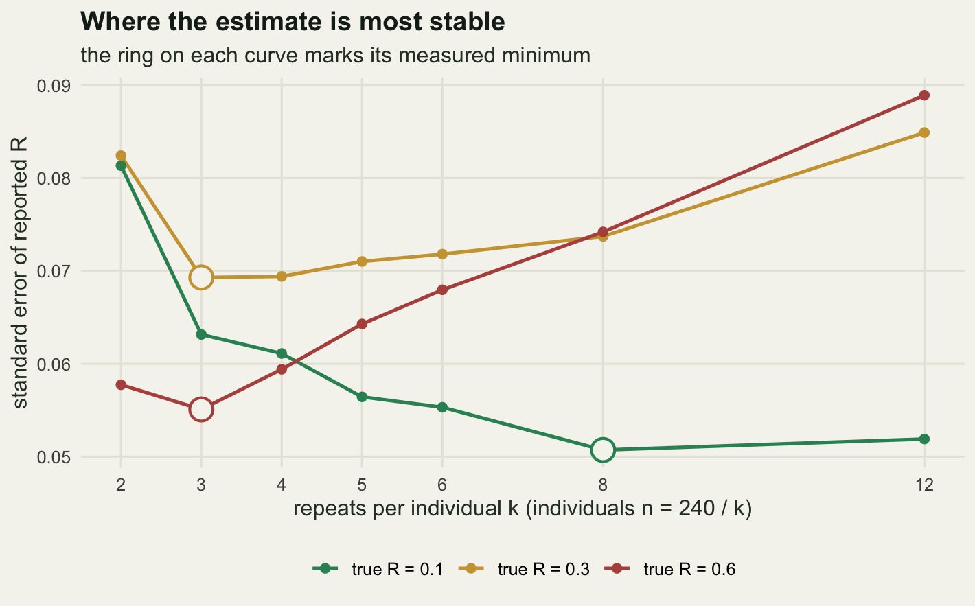
The measured minima sit at 8, 3 and 3 repeats for true repeatabilities of 0.1, 0.3 and 0.6. So the advice is right for the two higher values and wrong for the low one. For a weakly repeatable trait the best design in this grid was 8 repeats on 30 individuals, which is close to the opposite of what the rule says to do.
There is an algebraic reason and it is short enough to state. The large-sample variance of the intraclass correlation is proportional to \((1 + (k-1)R)^2 / (k(k-1)(n-1))\). Substituting \(n = N/k\) for a fixed total \(N\) cancels the k in the numerator of the denominator, leaving \((1 + (k-1)R)^2 / (k-1)\), and setting the derivative of that to zero gives \(k = 1 + 1/R\). The k_algebra column above is that expression evaluated at each true value: 11.0000, 4.3333 and 2.6667. The measurement and the algebra agree on the direction and, for the two higher true values, roughly on the location. At the low end the measured optimum (8) falls short of the algebraic one (11.0000), which is what you would expect when the curve is nearly flat over that whole region and eight hundred replicates cannot separate neighbouring cells.
The rule of thumb has quietly assumed that R is somewhere around the middle of its range, which is where most published behavioural repeatabilities sit, and it drifts off the optimum on either side of that. But the size of the drift is the part that matters, and it turns out to be smaller than the paragraphs above would lead you to expect.
The cost_of_k3 and cost_of_k4 columns are the ratios of the standard error at three and at four repeats to the standard error at the measured optimum for that row. The worst case anywhere in the grid is 1.2452 for three repeats and 1.2049 for four, both of them at the weakly repeatable trait. In other words, following the rule when the rule is wrong inflates the standard error by about a quarter at worst, and following the three-repeat half of it when the rule is right costs nothing at all, while four repeats costs 8 per cent at a true R of 0.6. The optimum is real, it moves with the true value in the direction the algebra predicts, and it is shallow enough that a design near three or four repeats is never a disaster.
Where the design does hurt is at the ends of the grid. With two repeats and a weakly repeatable trait, the raw estimator went negative and had to be truncated in 0.1500 of replicate studies, so that fraction of a hypothetical literature would report a flat zero for a trait that genuinely varies among individuals. At twelve repeats with a strongly repeatable trait the standard error is 0.0889 against 0.0551 at three repeats, and it is worse simply because twenty individuals is not many individuals. Both failures are about the number of individuals, one of them indirectly.
The practical reading. If you expect a weak signal, extra repeats per individual buy real precision and the standard advice will cost you a little. If you expect a strong signal, lean towards individuals: three repeats, not twelve. If you have no expectation at all, four repeats is a defensible hedge, because across every true value tested here its standard error was at most 1.2049 times the best available one.
Check two: how far apart were the repeats
A repeatability is not a property of a trait. It is a property of a trait and an interval. Two boldness scores taken twenty minutes apart share whatever the animal’s state was that morning; two taken three years apart share only what is stable across three years, and those are different quantities travelling under the same name and the same symbol.
Model that by letting each individual’s mean drift instead of holding it fixed. An Ornstein-Uhlenbeck process does it with one parameter: the individual deviate at the second measurement equals the first, shrunk by a factor that decays exponentially with the gap, plus fresh noise scaled to keep the total individual variance constant over time. The drift timescale is the parameter, and the repeatability you measure is the instantaneous repeatability multiplied by the shrinkage factor at your gap.
set.seed(20260729)
tau_days <- 45
sd_ind <- 1; sd_err <- 1
R_instant <- sd_ind^2 / (sd_ind^2 + sd_err^2)
n_b <- 200; reps_b <- 300

icc_pair <- function(gap, n, reps) {
  rho <- exp(-gap / tau_days)
  out <- numeric(reps)
  for (r in seq_len(reps)) {
    a1 <- rnorm(n, 0, sd_ind)
    a2 <- rho * a1 + rnorm(n, 0, sd_ind * sqrt(1 - rho^2))
    Y <- cbind(a1, a2) + matrix(rnorm(2 * n, 0, sd_err), n, 2)
    out[r] <- icc_balanced(Y)
  }
  mean(out)
}

gaps_head <- c(0.02, 21, 1095)
gap_names <- c("30 minutes", "3 weeks", "3 years")
R_head <- vapply(gaps_head, icc_pair, numeric(1), n = n_b, reps = reps_b)
names(R_head) <- gap_names
print(round(c(tau_true = tau_days, R_instant = R_instant,
              n_individuals = n_b, replicates = reps_b), 4))
tau_true R_instant n_individuals replicates
45.0 0.5 200.0 300.0 print(round(R_head, 4))30 minutes 3 weeks 3 years
0.4947 0.3129 -0.0059 tau_from_gap <- -gaps_head / log(pmax(R_head / R_instant, 1e-8))
names(tau_from_gap) <- gap_names
print(round(tau_from_gap, 2))30 minutes 3 weeks 3 years
1.88 44.80 59.44 One simulated process, measured three ways, gives 0.4947 at half an hour, 0.3129 at three weeks and -0.0059 at three years. The last of those is the raw estimator averaging fractionally below zero, which is its way of saying there is no detectable individual variance left. Same animals, same trait, same estimator, same code. A meta-analysis that pools the first value and the third is averaging two different quantities, and the distance between them is larger than most of the biological contrasts such analyses are built to detect.
The second chunk inverts the decay, recovering the drift timescale from each single estimate. From the three-week gap it returns 44.80 days against a true 45.0, which is close enough to be useful. From the half-hour gap it returns 1.88 days, which is nonsense, and the reason is worth sitting with: at a gap of 0.02 days the shrinkage factor is indistinguishable from one, so the logarithm in the denominator is taking the log of a quantity that is one plus noise, and dividing a small gap by a near-zero logarithm gives whatever the noise felt like. A short-gap study contains no information about how fast individuals drift. It cannot, and no amount of sample size at that one gap will change it.
set.seed(20260802)
gaps_curve <- c(0.02, 1, 3, 7, 14, 21, 45, 90, 180, 365, 730, 1095)
reps_curve <- 150
R_curve <- vapply(gaps_curve, icc_pair, numeric(1), n = n_b, reps = reps_curve)
curve_b <- data.frame(gap = gaps_curve, R = R_curve,
                      predicted = R_instant * exp(-gaps_curve / tau_days))
print(round(curve_b, 4))
gap R predicted
1 0.02 0.4981 0.4998
2 1.00 0.4968 0.4890
3 3.00 0.4723 0.4678
4 7.00 0.4262 0.4280
5 14.00 0.3732 0.3663
6 21.00 0.3142 0.3135
7 45.00 0.1702 0.1839
8 90.00 0.0636 0.0677
9 180.00 0.0053 0.0092
10 365.00 -0.0049 0.0002
11 730.00 -0.0096 0.0000
12 1095.00 -0.0036 0.0000print(round(c(replicates_per_gap = reps_curve,
max_gap_to_prediction = max(abs(curve_b$R - curve_b$predicted))), 4)) replicates_per_gap max_gap_to_prediction
150.0000 0.0138 head_b <- data.frame(gap = gaps_head, R = as.numeric(R_head), lab = gap_names)
head_b$lab_x <- c(gaps_head[1], 11, gaps_head[3])
head_b$lab_y <- c(head_b$R[1] + 0.075, 0.225, head_b$R[3] + 0.085)
head_b$hj <- c(0, 1, 1)
long_b <- rbind(data.frame(gap = curve_b$gap, R = curve_b$R, series = "measured"),
data.frame(gap = curve_b$gap, R = curve_b$predicted,
series = "exponential decay, tau = 45 days"))
ggplot(long_b, aes(gap, R, colour = series, linetype = series, linewidth = series)) +
geom_line() +
geom_point(data = long_b[long_b$series == "measured", ], size = 2,
show.legend = FALSE) +
annotate("segment", x = 12.5, xend = 19.5, y = 0.238, yend = 0.300,
colour = te_pal$ink, linewidth = 0.35) +
geom_text(data = head_b, aes(lab_x, lab_y, label = lab), inherit.aes = FALSE,
hjust = head_b$hj, size = 3.4, colour = te_pal$ink) +
scale_x_log10(breaks = c(0.02, 1, 7, 30, 180, 1095),
labels = c("0.02", "1", "7", "30", "180", "1095")) +
scale_colour_manual(values = c(te_pal$clay, te_pal$green), name = NULL) +
scale_linetype_manual(values = c(2, 1), name = NULL) +
scale_linewidth_manual(values = c(1.6, 0.7), name = NULL) +
coord_cartesian(ylim = c(-0.06, 0.62)) +
labs(title = "Repeatability decays with the gap between repeats",
x = "gap between the two repeats (days, log scale)",
y = "measured R") +
theme_te()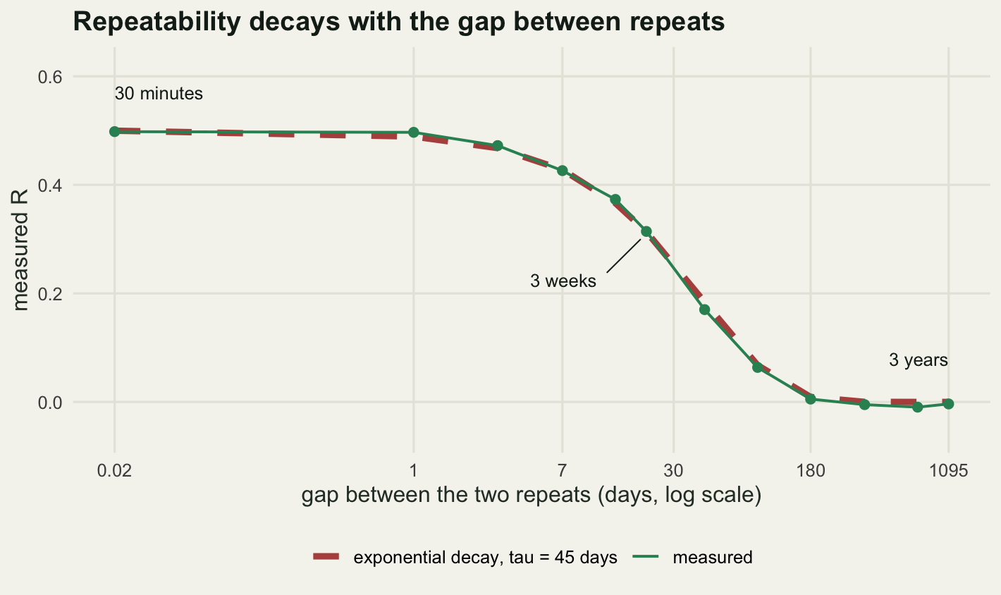
Across the twelve gaps the measured curve and the exponential prediction never differ by more than 0.0138, which is inside the Monte Carlo noise of 150 replicates per point. The decay is therefore not an artefact of the estimator misbehaving over long gaps: it is the process, seen through an estimator that is doing its job correctly at every gap.
Two things follow for a real study. Report the interval alongside the value, always, in the same sentence: 0.3129 over a three-week interval is a result, while the same number on its own is a quantity with a missing unit. And if the question is whether individuals differ in a stable way, one gap cannot answer it. Two or three well-separated gaps identify the timescale, and the timescale is usually the more interesting parameter, because it is what separates a mood from a trait.
This also explains a pattern that looks like publication bias and is not. Studies on short-lived animals, or studies run inside a single field season, will systematically report higher repeatabilities than studies that follow the same species across years. The gap is confounded with the study design, the study design is confounded with the taxon, and the resulting between-study variation in R has a mechanical component that no amount of careful meta-analysis coding will remove unless the interval is coded as a moderator.
Check three: who held the stopwatch
Here is the design that happens by accident rather than by decision. Two field assistants split the nest boxes geographically, so each bird is nearly always scored by the same person. If the two assistants differ at all in how they read the stopwatch, that difference is now attached to the individual, and the estimator has no way to tell the observer apart from the bird.
Simulate it with three variance components: individual, observer and residual. The target is the observer-adjusted repeatability, individual variance over individual plus residual, because the observer is a nuisance you want to condition away rather than a real source of among-individual difference. The unadjusted repeatability, with observer variance left in the denominator, is a different and smaller quantity, and keeping both in view turns out to matter.
n_c <- 30; k_c <- 4; m_c <- 6
va_c <- 0.30; vo_c <- 0.25; ve_c <- 0.70
p_primary <- 0.85
R_adjusted <- va_c / (va_c + ve_c)
R_unadjusted <- va_c / (va_c + vo_c + ve_c)
print(round(c(individuals = n_c, repeats = k_c, observers = m_c,
              var_ind = va_c, var_obs = vo_c, var_resid = ve_c,
              share_primary = p_primary,
              R_adjusted = R_adjusted, R_unadjusted = R_unadjusted), 4))
individuals repeats observers var_ind var_obs
30.00 4.00 6.00 0.30 0.25
var_resid share_primary R_adjusted R_unadjusted
0.70 0.85 0.30 0.24 icc_long <- function(y, ind, n, k) {
ind_mean <- as.vector(rowsum(y, ind)) / k
msb <- k * sum((ind_mean - mean(ind_mean))^2) / (n - 1)
msw <- sum((y - ind_mean[ind])^2) / (n * (k - 1))
(msb - msw) / (msb + (k - 1) * msw)
}
assign_confounded <- function(n, k, m, share = p_primary) {
primary <- rep(seq_len(m), length.out = n)
out <- integer(n * k)
for (i in seq_len(n)) {
swap <- runif(k) >= share
alt <- sample(setdiff(seq_len(m), primary[i]), k, replace = TRUE)
out[((i - 1) * k + 1):(i * k)] <- ifelse(swap, alt, primary[i])
}
out
}
assign_rotated <- function(n, k, m) {
as.integer(sapply(seq_len(n), function(i) sample(m, k)))
}
sim_observer <- function(n, k, m, obs) {
ind <- rep(seq_len(n), each = k)
a <- rnorm(n, 0, sqrt(va_c)); o <- rnorm(m, 0, sqrt(vo_c))
list(y = a[ind] + o[obs] + rnorm(n * k, 0, sqrt(ve_c)), ind = ind, obs = obs)
}The confounded design gives each individual a primary observer who scores a share 0.85 of its repeats, with the remainder scattered across the other observers. The rotated design draws 4 distinct observers for each individual from the 6 available, so no observer is attached to any particular animal. Same animals, same variance components, different assignment sheet.
The modelling fix needs a mixed model with two crossed random effects, and because this blog writes its own, here it is. The covariance matrix is the individual incidence matrix times its transpose, scaled by a variance ratio, plus the same construction for observer, plus the identity. Scaling everything by the residual variance leaves only two ratios to search over. The mean comes out by generalised least squares inside the objective, and the residual variance profiles out analytically, so optim only ever sees two free parameters.
neg_ll <- function(p, K_ind, K_obs, X, N) {
  ra <- exp(p[1]); ro <- exp(p[2])
  V <- ra * K_ind + ro * K_obs
  diag(V) <- diag(V) + 1
  ch <- chol(V)
  S <- backsolve(ch, X, transpose = TRUE)
  mu <- sum(S[, 1] * S[, 2]) / sum(S[, 2]^2)
  q <- sum((S[, 1] - mu * S[, 2])^2)
  0.5 * (2 * sum(log(diag(ch))) + N * log(q / N) + N)
}

fit_crossed <- function(d) {
  N <- length(d$y)
  K_ind <- outer(d$ind, d$ind, "==") * 1
  K_obs <- outer(d$obs, d$obs, "==") * 1
  X <- cbind(d$y, 1)
  opt <- optim(c(log(0.4), log(0.3)), neg_ll, K_ind = K_ind, K_obs = K_obs,
               X = X, N = N, method = "Nelder-Mead",
               control = list(maxit = 200, reltol = 1e-7))
  ra <- exp(opt$par[1]); ro <- exp(opt$par[2])
  V <- ra * K_ind + ro * K_obs
  diag(V) <- diag(V) + 1
  ch <- chol(V)
  S <- backsolve(ch, X, transpose = TRUE)
  mu <- sum(S[, 1] * S[, 2]) / sum(S[, 2]^2)
  s2 <- sum((S[, 1] - mu * S[, 2])^2) / N
  c(var_ind = ra * s2, var_obs = ro * s2, var_resid = s2, R = ra / (ra + 1))
}set.seed(20260730)
reps_c <- 150
conf_icc <- rot_icc <- conf_mod <- rot_mod <- numeric(reps_c)
va_hat <- vo_hat <- numeric(reps_c)
for (r in seq_len(reps_c)) {
d_conf <- sim_observer(n_c, k_c, m_c, assign_confounded(n_c, k_c, m_c))
conf_icc[r] <- icc_long(d_conf$y, d_conf$ind, n_c, k_c)
f <- fit_crossed(d_conf)
conf_mod[r] <- f["R"]; va_hat[r] <- f["var_ind"]; vo_hat[r] <- f["var_obs"]
d_rot <- sim_observer(n_c, k_c, m_c, assign_rotated(n_c, k_c, m_c))
rot_icc[r] <- icc_long(d_rot$y, d_rot$ind, n_c, k_c)
rot_mod[r] <- fit_crossed(d_rot)["R"]
}
means_c <- c(mean(conf_icc), mean(rot_icc), mean(conf_mod), mean(rot_mod))
res_c <- data.frame(
design = c("confounded, plain ICC", "rotated, plain ICC",
"confounded, observer in model", "rotated, observer in model"),
mean_R = means_c,
sd_R = c(sd(conf_icc), sd(rot_icc), sd(conf_mod), sd(rot_mod)),
bias = means_c - R_adjusted,
abs_bias = abs(means_c - R_adjusted))
print(round(c(replicates = reps_c), 0))replicates
150 print(data.frame(design = res_c$design, round(res_c[, -1], 4))) design mean_R sd_R bias abs_bias
1 confounded, plain ICC 0.3647 0.1008 0.0647 0.0647
2 rotated, plain ICC 0.2081 0.0978 -0.0919 0.0919
3 confounded, observer in model 0.2928 0.0990 -0.0072 0.0072
4 rotated, observer in model 0.2873 0.0976 -0.0127 0.0127print(round(c(var_ind_true = va_c, var_ind_fitted = mean(va_hat),
var_obs_true = vo_c, var_obs_fitted = mean(vo_hat),
lower_q = 0.025, upper_q = 0.975), 4)) var_ind_true var_ind_fitted var_obs_true var_obs_fitted lower_q
0.3000 0.2976 0.2500 0.2153 0.0250
upper_q
0.9750 qs_c <- rbind(quantile(conf_icc, c(0.025, 0.975), names = FALSE),
quantile(rot_icc, c(0.025, 0.975), names = FALSE),
quantile(conf_mod, c(0.025, 0.975), names = FALSE),
quantile(rot_mod, c(0.025, 0.975), names = FALSE))
plot_c <- data.frame(design = factor(res_c$design, levels = rev(res_c$design)),
mean_R = res_c$mean_R, lo = qs_c[, 1], hi = qs_c[, 2],
fix = c("no fix", "design fix", "modelling fix",
"design and modelling fix"))
plot_c$fix <- factor(plot_c$fix, levels = c("no fix", "design fix",
"modelling fix",
"design and modelling fix"))
ggplot(plot_c, aes(mean_R, design, colour = fix, shape = fix)) +
geom_vline(xintercept = R_adjusted, colour = te_pal$ink, linetype = 2, linewidth = 0.6) +
geom_vline(xintercept = R_unadjusted, colour = te_pal$ink, linetype = 3, linewidth = 0.6) +
geom_errorbar(aes(xmin = lo, xmax = hi), orientation = "y", width = 0.22, linewidth = 0.8) +
geom_point(size = 3) +
annotate("text", x = R_unadjusted - 0.008, y = 4.8, label = "unadjusted target",
hjust = 1, size = 3.1, colour = te_pal$ink) +
annotate("text", x = R_adjusted + 0.008, y = 4.8, label = "adjusted target",
hjust = 0, size = 3.1, colour = te_pal$ink) +
scale_y_discrete(expand = expansion(add = c(0.6, 1.25))) +
scale_colour_manual(values = c(te_pal$clay, te_pal$gold, te_pal$green, te_pal$forest),
name = NULL) +
scale_shape_manual(values = c(16, 17, 15, 18), name = NULL) +
guides(colour = "none", shape = "none") +
labs(title = "What the observer does to R",
x = "repeatability", y = NULL) +
theme_te() +
theme(plot.margin = margin(6, 16, 6, 6))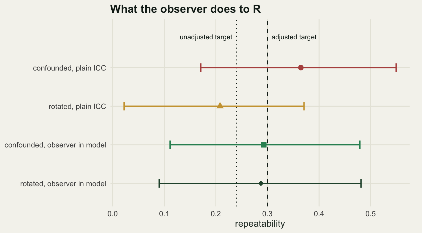
The confounded design returns 0.3647 against a target of 0.30, an inflation of 0.0647. That is the expected failure, and its size is the part to hold on to: an observer variance of 0.25 against an individual variance of 0.30 moved the headline number by 0.0647, with the observer only partly confounded rather than fully, in a design with 6 observers rather than the two that a real field season often has.
The surprise is the rotated design. Rotating observers across individuals removes the inflation and then overshoots in the other direction: the plain ICC on rotated data gives 0.2081, which is 0.0919 below the adjusted target and further from it than the confounded estimate was on the other side. That is not a bug in the rotation. Rotation moves the observer variance out of the between-individual term and into the within-individual term, so a plain ICC computed on rotated data is estimating individual variance over a total that still contains observer variance. That quantity is the unadjusted repeatability, 0.24, and the measured 0.2081 sits a little below even that, because drawing 4 distinct observers from a pool of 6 without replacement makes the observer contributions within one individual mildly anticorrelated and shaves the between-individual mean square further.
So the design fix and the modelling fix are not two roads to the same number. Rotation removes the confounding and hands you a clean estimate of a different estimand. Fitting observer as a random effect on the confounded data gives 0.2928, within 0.0072 of the target, and on rotated data it gives 0.2873. Only the model-based rows are estimating the quantity that most papers mean when they write repeatability, and the difference between the two model-based rows is small enough to be Monte Carlo noise at 150 replicates.
There is a residual downward bias in the model-based estimates and its source is visible in the variance components. The fitted observer variance averages 0.2153 against a true 0.25, a clear underestimate, because the observer pool has only 6 members and maximum likelihood shrinks a variance component estimated from that few levels. The fitted individual variance averages 0.2976 against 0.30, which is only modestly biased. Observer variance that the model fails to find stays in the residual, and residual variance sits in the denominator of R, so the estimate comes out slightly low. With a smaller observer pool this would be worse; with a larger one it would mostly disappear.
The one-line version. Rotation is a design fix, it is the cheaper of the two, and it changes what you are estimating. Observer as a random effect is a modelling fix, it keeps the estimand, and it needs enough observers to be worth fitting. The two fixes are not interchangeable, and the last row shows that the combination lands in the same place as the model alone rather than compounding.
Check four: the boundary at zero
A repeatability cannot be negative, and its estimator can be. When the true value is small, a sizeable fraction of studies produce a raw estimate below zero, report zero instead, and the sampling distribution of what gets reported develops a spike sitting on the boundary. Standard interval methods assume the estimate wanders symmetrically around the truth, and next to a wall it cannot.
Three intervals go head to head. The naive one takes the plug-in large-sample standard error and adds and subtracts 1.96 of them. The parametric bootstrap simulates fresh studies from the fitted values and takes the 0.025 and 0.975 quantiles of the resulting estimates. The likelihood-ratio interval collects every value of R whose profile deviance is within the chi-squared threshold of the minimum. For a balanced design the profile deviance has a closed form after concentrating out the total variance, which is what makes it cheap enough to run several hundred times at each grid point.
n_d <- 30; k_d <- 3
df_b <- n_d - 1; df_w <- n_d * (k_d - 1); df_tot <- df_b + df_w
z_norm <- 1.96; nominal <- 0.95

ss_of <- function(Y) {
  row_mean <- rowMeans(Y)
  c(k_d * sum((row_mean - mean(row_mean))^2), sum((Y - row_mean)^2))
}
icc_from_ss <- function(s) {
  msb <- s[1] / df_b; msw <- s[2] / df_w
  (msb - msw) / (msb + (k_d - 1) * msw)
}
deviance_R <- function(R, s) {
  if (R < 0 || R >= 1) return(Inf)
  a <- 1 + (k_d - 1) * R; b <- 1 - R
  v <- (s[1] / a + s[2] / b) / df_tot
  df_tot * log(v) + df_b * log(a) + df_w * log(b)
}
profile_min <- function(s) {
  Rh <- max(0, icc_from_ss(s))
  c(Rh, deviance_R(Rh, s))
}
lr_interval <- function(s, crit = qchisq(nominal, 1)) {
  pm <- profile_min(s); Rh <- pm[1]; d0 <- pm[2]
  f <- function(R) deviance_R(R, s) - d0 - crit
  lo <- if (f(0) <= 0) 0 else uniroot(f, c(0, Rh), tol = 1e-7)$root
  hi <- if (f(0.9999) <= 0) 0.9999 else uniroot(f, c(max(Rh, 1e-9), 0.9999), tol = 1e-7)$root
  c(lo, hi)
}
se_plugin <- function(R) {
  sqrt(2 * (1 - R)^2 * (1 + (k_d - 1) * R)^2 / (k_d * (k_d - 1) * (n_d - 1)))
}
boot_icc <- function(Rh, n, k, B) {
  Y <- matrix(rnorm(n * k * B, 0, sqrt(1 - Rh)), n, k * B)
  ab <- matrix(rnorm(n * B, 0, sqrt(Rh)), n, B)
  Y <- Y + ab[, rep(seq_len(B), each = k)]
  idx <- lapply(seq_len(k), function(j) seq(j, k * B, by = k))
  row_mean <- 0
  for (j in seq_len(k)) row_mean <- row_mean + Y[, idx[[j]], drop = FALSE]
  row_mean <- row_mean / k
  ssb <- k * colSums((row_mean - rep(colMeans(row_mean), each = n))^2)
  ssw <- 0
  for (j in seq_len(k)) ssw <- ssw + colSums((Y[, idx[[j]], drop = FALSE] - row_mean)^2)
  msb <- ssb / (n - 1); msw <- ssw / (n * (k - 1))
  pmax(0, (msb - msw) / (msb + (k - 1) * msw))
}
print(round(c(individuals = n_d, repeats = k_d, nominal = nominal,
              z_norm = z_norm, lower_q = 0.025, upper_q = 0.975,
              chisq_crit = qchisq(nominal, 1), boundary_theory = 0.5), 4))
individuals repeats nominal z_norm lower_q
30.0000 3.0000 0.9500 1.9600 0.0250
upper_q chisq_crit boundary_theory
0.9750 3.8415 0.5000 The bootstrap is the expensive part of that grid, so boot_icc generates every resampled study for one dataset in a single matrix rather than looping. Each column block of k columns is one bootstrap study, the individual deviates are recycled across the block, and the two sums of squares come out of a handful of colSums calls. It is the same arithmetic as icc_balanced, arranged so that R does the loop in C, and it is what keeps this section inside the knit budget.
set.seed(20260731)
R_grid_d <- c(0, 0.05, 0.10, 0.20, 0.40, 0.70)
reps_d <- 600; n_boot <- 199
cover_d <- NULL
for (Rt in R_grid_d) {
  miss <- matrix(0, 3, 2); at_zero <- 0; neg_lower <- 0
  for (r in seq_len(reps_d)) {
    s <- ss_of(sim_balanced(n_d, k_d, Rt))
    R_raw <- icc_from_ss(s); Rh <- max(0, R_raw)
    at_zero <- at_zero + (R_raw <= 0)
    half <- z_norm * se_plugin(Rh)
    neg_lower <- neg_lower + (Rh - half < 0)
    miss[1, ] <- miss[1, ] + c(Rh - half > Rt, Rh + half < Rt)
    boot <- boot_icc(Rh, n_d, k_d, n_boot)
    qb <- quantile(boot, c(0.025, 0.975), names = FALSE)
    miss[2, ] <- miss[2, ] + c(qb[1] > Rt, qb[2] < Rt)
    ci <- lr_interval(s)
    miss[3, ] <- miss[3, ] + c(ci[1] > Rt, ci[2] < Rt)
  }
  cover_d <- rbind(cover_d, data.frame(
    R_true = Rt, at_zero = at_zero / reps_d, neg_lower = neg_lower / reps_d,
    naive = 1 - sum(miss[1, ]) / reps_d,
    bootstrap = 1 - sum(miss[2, ]) / reps_d,
    likelihood = 1 - sum(miss[3, ]) / reps_d))
}
print(round(c(replicates = reps_d, bootstrap_draws = n_boot), 0))
replicates bootstrap_draws
600 199 print(round(cover_d, 4)) R_true at_zero neg_lower naive bootstrap likelihood
1 0.00 0.5017 0.9783 0.9783 0.9800 0.9767
2 0.05 0.3667 0.9517 0.9783 0.9800 0.9733
3 0.10 0.1950 0.8850 0.9817 0.9867 0.9717
4 0.20 0.0417 0.6333 0.9850 0.9783 0.9633
5 0.40 0.0000 0.0767 0.9500 0.9500 0.9550
6 0.70 0.0000 0.0000 0.9283 0.9317 0.9400print(round(c(mc_se_of_coverage = sqrt(nominal * (1 - nominal) / reps_d),
max_bootstrap_minus_naive = max(abs(cover_d$bootstrap - cover_d$naive))), 4)) mc_se_of_coverage max_bootstrap_minus_naive
0.0089 0.0067 long_d <- rbind(
data.frame(R_true = cover_d$R_true, coverage = cover_d$naive, series = "naive normal"),
data.frame(R_true = cover_d$R_true, coverage = cover_d$bootstrap,
series = "parametric bootstrap"),
data.frame(R_true = cover_d$R_true, coverage = cover_d$likelihood,
series = "likelihood ratio"))
long_d$series <- factor(long_d$series,
levels = c("naive normal", "parametric bootstrap",
"likelihood ratio"))
ggplot(long_d, aes(R_true, coverage, colour = series)) +
geom_hline(yintercept = nominal, linetype = 2, colour = te_pal$ink, linewidth = 0.6) +
geom_line(linewidth = 0.9) +
geom_point(size = 2.2) +
scale_colour_manual(values = c(te_pal$green, te_pal$gold, te_pal$clay), name = NULL) +
scale_x_continuous(breaks = R_grid_d) +
labs(title = "Coverage of three intervals for R",
x = "true repeatability", y = "measured coverage") +
theme_te()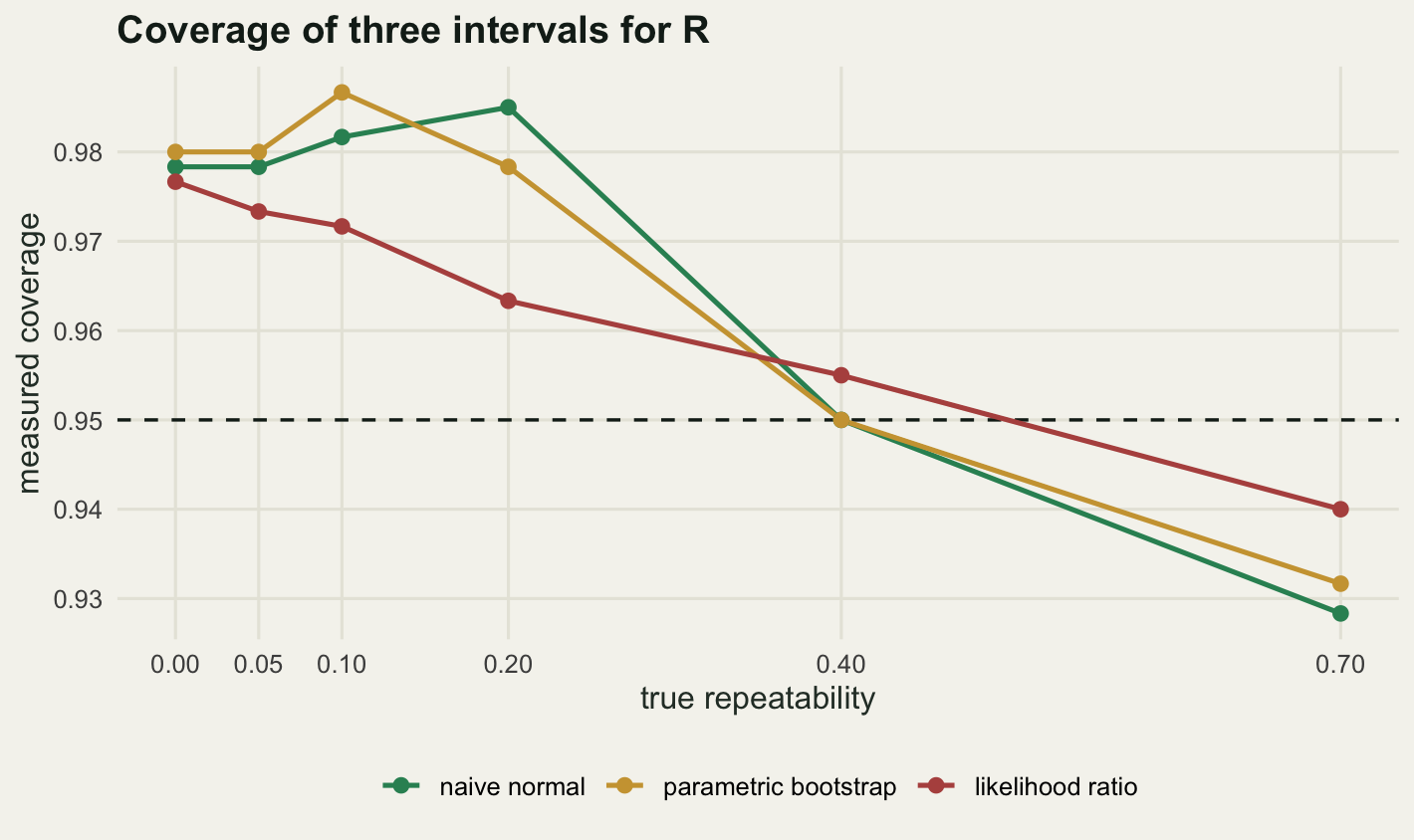
Start with the boundary itself. At a true R of zero the raw estimator came out at or below zero in 0.5017 of studies, against the theoretical 0.5, and the proportion falls to 0.3667 at a true R of 0.05 and 0.1950 at 0.10. With thirty individuals and three repeats, a genuinely weak but non-zero repeatability is reported as a flat zero in a meaningful fraction of studies, and those are exactly the studies least likely to be written up at all.
Now the intervals, and this is where the plan I started with was wrong. The expectation was that the naive normal interval would undercover near the boundary. It does not. At the four smallest true values its measured coverage is 0.9783, 0.9783, 0.9817 and 0.9850, every one of them above the nominal 0.95. It overcovers, and it overcovers by cheating: its lower limit is below zero in 0.9783 of studies at a true R of zero, and still 0.6333 at a true R of 0.20. An interval that reaches into impossible territory will of course contain the truth more often than advertised. That is not conservatism in any useful sense: it is a reported range of which a large part cannot occur.
Truncating the naive interval at zero, which is what any careful person does before printing it, changes none of this. Every study whose lower limit was negative had a lower limit that still sits at or below the truth after truncation, so coverage is identical either way. The truncation removes the embarrassment and leaves the error.
The undercoverage is real, but it appears only once the true value has moved well away from the boundary, which is not where anyone goes looking for it. At a true R of 0.40 the three coverages are 0.9500 for the naive interval, 0.9500 for the bootstrap and 0.9550 for the likelihood ratio, and at 0.70 they are 0.9283, 0.9317 and 0.9400. The Monte Carlo standard error of a coverage estimate at this number of replicates is 0.0089, so a shortfall has to be about twice that before it counts as evidence, which is worth saying plainly rather than reading a two-point dip as a finding.
What survives that caution is an ordering rather than any single value. The likelihood-ratio interval is the only one of the three that never sits more than two Monte Carlo standard errors below nominal anywhere in the grid: its worst value is 0.9400, at the largest true R tested. The naive interval is the furthest below nominal at that same point, 0.9283, and the parametric bootstrap does not rescue the situation either, which was also not the expectation going in. Resampling from a truncated point estimate inherits the truncation, so at small true values the bootstrap distribution is itself piled up on the boundary, and its coverage tracks the analytic interval closely rather than improving on it: the two agree to within 0.0067 at every grid point.
set.seed(20260801)
reps_lrt <- 3000
alpha <- 0.05
stat_lrt <- numeric(reps_lrt)
for (r in seq_len(reps_lrt)) {
  s <- ss_of(sim_balanced(n_d, k_d, 0))
  stat_lrt[r] <- deviance_R(0, s) - profile_min(s)[2]
}
print(c(replicates = reps_lrt))
replicates
3000 print(round(c(alpha = alpha), 4))alpha
0.05 print(round(c(crit_chisq1 = qchisq(1 - alpha, 1), crit_mixture = qchisq(1 - 2 * alpha, 1),
error_chisq1 = mean(stat_lrt > qchisq(1 - alpha, 1)),
error_mixture = mean(stat_lrt > qchisq(1 - 2 * alpha, 1)),
prop_stat_zero = mean(stat_lrt <= 0)), 4)) crit_chisq1 crit_mixture error_chisq1 error_mixture prop_stat_zero
3.8415 2.7055 0.0243 0.0483 0.5067 The last piece is the test of R = 0 itself. Comparing the likelihood-ratio statistic against a chi-squared with one degree of freedom, the threshold 3.8415, is what a naive reading of any model comparison gives you, and across 3000 null datasets it produced a type I error rate of 0.0243 against a nominal 0.05. The test is conservative by roughly a factor of two, and the reason is in the next printed number: the statistic was exactly zero in 0.5067 of null datasets, because half of the time the estimate is already sitting on the boundary and there is no likelihood to be gained by moving off it.
The correct null distribution is therefore an even mixture of a point mass at zero and a chi-squared with one degree of freedom. Half the mass never exceeds any positive threshold, so the threshold that leaves 0.05 of the mixture in the upper tail is the one that leaves 0.1 of the plain chi-squared there, namely 2.7055. Using that value gives a measured error rate of 0.0483, which is what a test at 0.05 is supposed to do. The practical consequence runs opposite to most calibration problems: the naive test is too cautious, so it discards real among-individual variance rather than inventing it, and the studies it silences are the weakly repeatable ones that the meta-analysis most needs to see.
What to take away
Four checks, two of which came back against the plan they were written from. The design check said the rule of three or four repeats is right for moderate and high repeatabilities and wrong for low ones, where the measured optimum sat at 8 repeats, but it also said the penalty for following the rule anyway is at most 1.2452 times the best available standard error, which is a much weaker indictment than the section started out expecting. The boundary check said the naive interval overcovers rather than undercovers near zero, and that it does so by reporting negative lower limits, while the undercoverage that does exist lives out at the top of the range tested, where nobody thinks to look for it.
The other two behaved as expected in direction and were larger than expected in size. The interval between repeats moved the estimate from 0.4947 to -0.0059 on a single simulated process, which is the full range from a strong result to nothing. Observer confounding moved it by 0.0647 upwards, and the obvious design fix moved it 0.0919 downwards past the target rather than onto it, because rotation changes the estimand instead of correcting the estimate.
The honest limit of all of this: every number above comes from a Gaussian, balanced, correctly specified simulation, so what has been measured is how the estimator behaves when the model it assumes is exactly true, and a real repeatability analysis usually breaks one of those assumptions before it gets anywhere near the four issues studied here. Counts and proportions, unequal numbers of repeats, individuals that drop out because they died, and traits that change with age all alter the arithmetic in ways this post does not touch, and the sizes quoted here should be read as directions with a rough scale rather than as corrections to apply.
What does survive is enough to act on, and none of it needs a bigger dataset. Report the interval between repeats in the same sentence as the value. Say who scored what, and if the answer is that one person mostly scored one set of animals, fit observer as a random effect rather than rotating and hoping. Prefer a likelihood-ratio interval to an estimate plus or minus two standard errors, and if the estimate is near zero, test it against the mixture rather than the plain chi-squared. Every one of those is a decision about the analysis, not about the budget, and each of them was measured above against a truth that was known in advance.
References
Nakagawa S, Schielzeth H 2010 Biological Reviews 85(4):935-956 (10.1111/j.1469-185X.2010.00141.x)
Bell AM, Hankison SJ, Laskowski KL 2009 Animal Behaviour 77(4):771-783 (10.1016/j.anbehav.2008.12.022)
Araya-Ajoy YG, Mathot KJ, Dingemanse NJ 2015 Methods in Ecology and Evolution 6(12):1462-1473 (10.1111/2041-210X.12430)
Dingemanse NJ, Dochtermann NA 2013 Journal of Animal Ecology 82(1):39-54 (10.1111/1365-2656.12013)
Stoffel MA, Nakagawa S, Schielzeth H 2017 Methods in Ecology and Evolution 8(11):1639-1644 (10.1111/2041-210X.12797)
Self SG, Liang KY 1987 Journal of the American Statistical Association 82(398):605-610 (10.1080/01621459.1987.10478472)