library(ggplot2)

te_pal <- list(forest = "#275139", green = "#2f8f63", sage = "#93a87f",
               clay = "#b5534e", gold = "#cda23f", line = "#dad9ca",
               ink = "#16241d", paper = "#f5f4ee")

theme_te <- function() {
  theme_minimal(base_size = 12) +
    theme(panel.grid.minor = element_blank(),
          panel.grid.major = element_line(colour = "#e7e6dc"),
          plot.background = element_rect(fill = "#f5f4ee", colour = NA),
          panel.background = element_rect(fill = "#f5f4ee", colour = NA),
          plot.title = element_text(face = "bold", colour = te_pal$ink),
          axis.title = element_text(colour = "#2c3a31"))
}Checking an acoustic monitoring analysis
R
bioacoustics
acoustic monitoring
model diagnostics
ecology tutorial
ggplot2
Four diagnostics for automated acoustic monitoring in R: bout overdispersion, thresholds that fail to transfer between sites, duty cycles and validation effort.
An automated recogniser turns a night of audio into a table: a time, a score, sometimes a species label. The three earlier posts in this cluster built the analysis that sits on top of that table. Detections became a corrected index in Automated acoustic detections as data; a score cut was chosen against precision; call counts became a rate and then a density. Every one of those steps rests on an assumption about how calls arrive, how the recogniser behaves away from the site it was tuned on, and how well the correction factors are known.
This post measures four of those assumptions against simulated data where the truth is fixed and visible. Each check is self-contained: a simulator, a number, and the consequence for something an ecologist would actually report. Two of them behave as the textbook account says. One produces a standard fix that makes matters worse, and one overturns the received wisdom about recording schedules in both directions at once. The simulators are written by hand so that every constant is visible and every design number is printed rather than asserted; nothing here needs a package beyond ggplot2.
Bouts break the recorder-hour as a unit
Almost nothing calls at a constant rate. A bird sings, then sings again a few seconds later, then falls silent for twenty minutes. A bat forages through a patch and leaves. The result is a clustered point process: bout onsets arrive at random, and each onset drags a random number of cues behind it. The simulator below is a Neyman-Scott process in the crudest form. Bout onsets are Poisson in time, bout size is one plus a Poisson draw, and the cues in a bout are scattered over a short window. A plain Poisson process with the identical mean rate is the comparison.
set.seed(20260814)
n_rep <- 2000L
n_hours <- 12L
bout_rate <- 0.75
bout_mu <- 5
bout_spread <- 3
cue_rate <- bout_rate * (1 + bout_mu)
print(c(surveys = n_rep, recorder_hours = n_hours, bouts_per_hour = bout_rate,
        mean_bout_size = 1 + bout_mu, bout_window_minutes = bout_spread,
        cues_per_hour = cue_rate))
surveys recorder_hours bouts_per_hour mean_bout_size
2000.00 12.00 0.75 6.00
bout_window_minutes cues_per_hour
3.00 4.50 sim_bout_hours <- function(n_hours, bout_rate, bout_mu, bout_spread) {
span <- n_hours * 60
n_bouts <- rpois(1, bout_rate * (n_hours + bout_spread / 60))
if (n_bouts == 0L) return(integer(n_hours))
onset <- runif(n_bouts, -bout_spread, span)
sizes <- 1L + rpois(n_bouts, bout_mu)
cues <- rep(onset, sizes) + runif(sum(sizes), 0, bout_spread)
cues <- cues[cues >= 0 & cues < span]
tabulate(floor(cues / 60) + 1L, nbins = n_hours)
}The onsets start slightly before the survey window so that a bout straddling the first minute is represented. Without that warm-up the first block of every simulated night is quietly too empty, which biases anything that compares the start of a recording with the rest of it.
clus_counts <- t(replicate(n_rep, sim_bout_hours(n_hours, bout_rate, bout_mu, bout_spread)))
pois_counts <- matrix(rpois(n_rep * n_hours, cue_rate), nrow = n_rep)
vmr <- function(x) var(as.numeric(x)) / mean(as.numeric(x))

bin_len <- 60
mean_size <- 1 + bout_mu
mean_sq_size <- bout_mu + (1 + bout_mu)^2
# q(u) is the share of a bout's cues that land in the hour the onset sits in;
# the variance needs the integral of q(u)^2 over the hour, not just of q(u)
overlap <- (bin_len - bout_spread) + 2 * bout_spread / 3
vmr_whole_bout <- mean_sq_size / mean_size
vmr_expected <- (mean_size * (bin_len - overlap) + mean_sq_size * overlap) /
                (mean_size * bin_len)

# delete-one-night jackknife standard error of the simulated ratio
row_s <- rowSums(clus_counts)
row_q <- rowSums(clus_counts^2)
m_left <- length(clus_counts) - n_hours
s_left <- sum(row_s) - row_s
q_left <- sum(row_q) - row_q
jack <- ((q_left - s_left^2 / m_left) / (m_left - 1)) / (s_left / m_left)
vmr_se <- sqrt((n_rep - 1) / n_rep * sum((jack - mean(jack))^2))

print(round(c(mean_poisson = mean(pois_counts), mean_bouts = mean(clus_counts),
              vmr_poisson = vmr(pois_counts), vmr_bouts = vmr(clus_counts),
              vmr_whole_bout = vmr_whole_bout, vmr_expected = vmr_expected,
              vmr_jackknife_se = vmr_se,
              gap_in_se = (vmr(clus_counts) - vmr_expected) / vmr_se), 4))
mean_poisson mean_bouts vmr_poisson vmr_bouts
4.5130 4.4784 0.9964 6.8339
vmr_whole_bout vmr_expected vmr_jackknife_se gap_in_se
6.8333 6.7361 0.0651 1.5030 Both processes deliver about 4.5 cues per recorder-hour: the means are 4.5130 and 4.4784. The variance-to-mean ratio is 0.9964 for the Poisson counts and 6.8339 for the bout counts. The compound-Poisson algebra gives 6.8333 for a bout size with mean 6 and variance 5, but that value holds only if every bout falls inside one hourly bin. A bout scattered over a three-minute window sometimes straddles the boundary between two hours and is cut in two, which pulls the prediction down to 6.7361. A delete-one-night jackknife puts the standard error of the simulated ratio at 0.0651, so the simulation sits 1.5030 standard errors above the corrected prediction: the two agree to the precision two thousand simulated nights can support. Either way the bout process is not a little overdispersed. It carries almost seven times the variance of the Poisson process it is impersonating.
That ratio is a curiosity until it is attached to an interval. A survey of twelve recorder-hours yields a total count; the Poisson standard error of the rate is the square root of that total divided by the number of hours. Three intervals are compared here: that Poisson interval, a quasi-Poisson interval whose dispersion is estimated from the twelve hourly counts, and a bootstrap that resamples whole recorder-hours. Coverage is the fraction of simulated surveys whose interval contains the true rate.
n_boot <- 400L
covered <- function(counts) {
  total <- rowSums(counts)
  rate_hat <- total / n_hours
  se_pois <- sqrt(total) / n_hours
  phi <- apply(counts, 1, function(y) sum((y - mean(y))^2) / mean(y)) / (n_hours - 1)
  se_quasi <- sqrt(phi * rate_hat / n_hours)
  tq <- qt(0.975, n_hours - 1)
  hit_boot <- vapply(seq_len(nrow(counts)), function(i) {
    bs <- matrix(sample(counts[i, ], n_hours * n_boot, replace = TRUE), nrow = n_boot)
    lim <- quantile(rowMeans(bs), c(0.025, 0.975), names = FALSE)
    cue_rate >= lim[1] && cue_rate <= lim[2]
  }, logical(1))
  c(poisson_se = mean(abs(rate_hat - cue_rate) <= 1.96 * se_pois),
    quasi_se = mean(abs(rate_hat - cue_rate) <= tq * se_quasi),
    hour_bootstrap = mean(hit_boot),
    mean_width_poisson = mean(2 * 1.96 * se_pois),
    mean_width_quasi = mean(2 * tq * se_quasi))
}
cov_pois <- covered(pois_counts)
cov_clus <- covered(clus_counts)
print(c(bootstrap_resamples = n_boot, nominal_coverage = 0.95))
bootstrap_resamples nominal_coverage
400.00 0.95 print(round(rbind(poisson_process = cov_pois, bout_process = cov_clus), 4)) poisson_se quasi_se hour_bootstrap mean_width_poisson
poisson_process 0.9445 0.9415 0.912 2.3983
bout_process 0.5305 0.9160 0.890 2.3534
mean_width_quasi
poisson_process 2.6267
bout_process 6.7436print(round(c(se_inflation = sqrt(vmr(clus_counts)),
width_ratio = cov_clus[["mean_width_quasi"]] /
cov_clus[["mean_width_poisson"]]), 4))se_inflation width_ratio
2.6142 2.8655 The nominal 0.95 interval built from the Poisson standard error covers the truth 0.9445 of the time on Poisson data and 0.5305 of the time on bout data. An interval advertised as 95 per cent is a 53 per cent interval. The quasi-Poisson version recovers most of the loss, 0.9160, and the hour-level bootstrap reaches 0.8900 on bout data; both still fall short, because a dispersion estimated from twelve hours is itself noisy and twelve is a thin base for a percentile bootstrap. The mean interval width tells the same story from the other side: 2.3534 for the Poisson interval against 6.7436 for the quasi-Poisson interval on the same bout data, a ratio of 2.8655.
cov_dat <- data.frame(
  process = rep(c("Poisson process", "bout process"), each = 3),
  interval = rep(c("Poisson SE", "quasi-Poisson SE", "hour bootstrap"), 2),
  coverage = c(cov_pois[1:3], cov_clus[1:3]))
cov_dat$interval <- factor(cov_dat$interval,
                           c("Poisson SE", "quasi-Poisson SE", "hour bootstrap"))
cov_dat$process <- factor(cov_dat$process, c("Poisson process", "bout process"))

p_cov <- ggplot(cov_dat, aes(interval, coverage, fill = process)) +
  geom_col(position = position_dodge(width = 0.8), width = 0.7) +
  geom_hline(yintercept = 0.95, linetype = 2, colour = te_pal$clay) +
  scale_fill_manual(values = c("Poisson process" = te_pal$sage,
                               "bout process" = te_pal$forest)) +
  coord_cartesian(ylim = c(0, 1)) +
  labs(title = "A nominal 95 percent interval on bout-structured counts",
       x = NULL, y = "realised coverage", fill = NULL) +
  theme_te() + theme(legend.position = "top")
p_cov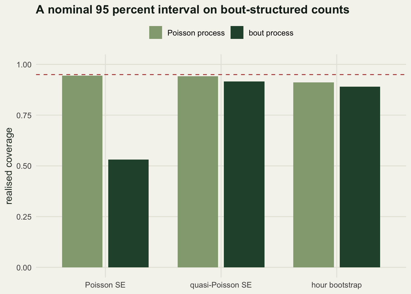
The lesson is a statement about units, not about distributions. The recorder-hour is not the independent unit of an acoustic survey; the bout is. Anything that treats hours, or minutes, or individual detections as independent replicates will report an interval that is too narrow by roughly the square root of the dispersion, which here is 2.6142.
A threshold tuned at one site does not travel
A recogniser score separates true calls from noise imperfectly. The usual practice is to listen to a sample of clips, find the score at which precision reaches some target, and use that score everywhere. The hidden assumption is that the noise score distribution is the same everywhere. It is not: a site near a stream, a road or a windy ridge produces higher-scoring rubbish.
Two sites are simulated with the same true call rate and different background noise. Scores for true calls are Normal around a fixed mean at both sites; noise scores are Normal around a site mean plus a nightly shift. The first eight nights at each site are the labelled validation nights, the remaining sixteen are the survey.
set.seed(4021)
n_nights <- 24L
n_val_nights <- 8L
hours_per_night <- 6L
call_rate <- 6
noise_rate <- 40
signal_mu <- 3.2
night_sd <- 0.4
target_prec <- 0.90
print(c(nights = n_nights, validation_nights = n_val_nights,
        hours_per_night = hours_per_night, calls_per_hour = call_rate,
        noise_per_hour = noise_rate, signal_mean = signal_mu,
        night_sd = night_sd, target_precision = target_prec))
nights validation_nights hours_per_night calls_per_hour
24.0 8.0 6.0 6.0
noise_per_hour signal_mean night_sd target_precision
40.0 3.2 0.4 0.9 sim_site <- function(label, noise_mu) {
night_shift <- rnorm(n_nights, 0, night_sd)
do.call(rbind, lapply(seq_len(n_nights), function(k) {
n_call <- rpois(1, call_rate * hours_per_night)
n_noise <- rpois(1, noise_rate * hours_per_night)
data.frame(site = label, night = k, noise_mean = noise_mu + night_shift[k],
truth = rep(c(1L, 0L), c(n_call, n_noise)),
score = c(rnorm(n_call, signal_mu, 1),
rnorm(n_noise, noise_mu + night_shift[k], 1)))
}))
}
d_all <- rbind(sim_site("quiet", 0), sim_site("noisy", 1))
d_all$phase <- ifelse(d_all$night <= n_val_nights, "val", "use")
thr_grid <- seq(0, 6, by = 0.01)
tune_thr <- function(sc, tr) {
pv <- vapply(thr_grid, function(s) {
keep <- sc >= s
if (sum(keep) < 10L) NA_real_ else mean(tr[keep])
}, numeric(1))
ok <- which(!is.na(pv) & pv >= target_prec)
if (length(ok)) thr_grid[min(ok)] else thr_grid[which.max(replace(pv, is.na(pv), -1))]
}
is_val <- d_all$phase == "val"
thr_q <- tune_thr(d_all$score[is_val & d_all$site == "quiet"],
d_all$truth[is_val & d_all$site == "quiet"])
thr_n <- tune_thr(d_all$score[is_val & d_all$site == "noisy"],
d_all$truth[is_val & d_all$site == "noisy"])
print(c(threshold_quiet = thr_q, threshold_noisy = thr_n))threshold_quiet threshold_noisy
2.86 3.86 The quiet site needs a score of 2.86 to reach 90 per cent precision; the noisy site needs 3.86. Now apply the quiet-site threshold at both, on the survey nights that were never used for tuning, and record what an analyst would see: a detection rate, a precision and a recall.
u_use <- d_all[d_all$phase == "use", ]
hrs_use <- (n_nights - n_val_nights) * hours_per_night
at_thr <- function(s_quiet, s_noisy) {
  a <- u_use$site == "quiet"
  b <- u_use$site == "noisy"
  ka <- u_use$score[a] >= s_quiet
  kb <- u_use$score[b] >= s_noisy
  c(rate_quiet = sum(ka) / hrs_use, rate_noisy = sum(kb) / hrs_use,
    ratio = sum(kb) / sum(ka),
    prec_quiet = mean(u_use$truth[a][ka]), prec_noisy = mean(u_use$truth[b][kb]),
    recall_quiet = sum(u_use$truth[a] == 1L & ka) / sum(u_use$truth[a]),
    recall_noisy = sum(u_use$truth[b] == 1L & kb) / sum(u_use$truth[b]))
}
seen <- rbind(one_threshold = at_thr(thr_q, thr_q), per_site = at_thr(thr_q, thr_n))
print(round(seen, 4))
rate_quiet rate_noisy ratio prec_quiet prec_noisy recall_quiet
one_threshold 4.3854 6.0208 1.3729 0.9857 0.6401 0.6587
per_site 4.3854 1.7083 0.3895 0.9857 0.8293 0.6587
recall_noisy
one_threshold 0.5968
per_site 0.2194truth_ratio <- sum(u_use$truth[u_use$site == "noisy"]) /
sum(u_use$truth[u_use$site == "quiet"])
print(round(c(true_rate_quiet = sum(u_use$truth[u_use$site == "quiet"]) / hrs_use,
true_rate_noisy = sum(u_use$truth[u_use$site == "noisy"]) / hrs_use,
true_ratio = truth_ratio,
bias_one_threshold = seen["one_threshold", "ratio"] - truth_ratio,
bias_per_site = seen["per_site", "ratio"] - truth_ratio), 4)) true_rate_quiet true_rate_noisy true_ratio bias_one_threshold
6.5625 6.4583 0.9841 0.3888
bias_per_site
-0.5946 With one threshold everywhere, precision is 0.9857 at the quiet site and 0.6401 at the noisy site: a third of the noisy site’s detections are rubbish. The detection rates are 4.3854 and 6.0208 per hour, so the noisy site looks 1.3729 times as active as the quiet one, against a realised truth of 0.9841. The ratio is off by 0.3888, and that spurious difference is the entire signal a naive comparison would report. It is a property of the microphone’s surroundings.
Recalibrating per site is the obvious fix, and it does not work. Tuning the noisy site to the same 90 per cent target lifts its threshold to 3.86, which brings precision to 0.8293 out of sample, but recall collapses from 0.6587 at the quiet site to 0.2194 at the noisy one. The detection rate falls to 1.7083 per hour and the apparent ratio becomes 0.3895, an error of -0.5946 where the one-threshold error was 0.3888. The spurious difference has not been removed; its sign has flipped and its size has grown. Equal precision buys unequal recall, and a detection count is proportional to recall.
night_key <- interaction(d_all$site, d_all$night, drop = TRUE)
thr_night <- tapply(seq_len(nrow(d_all)), night_key,
                    function(i) tune_thr(d_all$score[i], d_all$truth[i]))
use_key <- as.character(interaction(u_use$site, u_use$night, drop = TRUE))
kept_night <- u_use$score >= as.numeric(thr_night[use_key])
n_keep_q <- sum(kept_night & u_use$site == "quiet")
n_keep_n <- sum(kept_night & u_use$site == "noisy")
print(round(c(threshold_sd = sd(as.numeric(thr_night)),
              threshold_min = min(as.numeric(thr_night)),
              threshold_max = max(as.numeric(thr_night)),
              rate_quiet = n_keep_q / hrs_use, rate_noisy = n_keep_n / hrs_use,
              ratio = n_keep_n / n_keep_q), 4))
threshold_sd threshold_min threshold_max rate_quiet rate_noisy
0.7800 0.7900 4.2100 6.2188 3.0104
ratio
0.4841 # the threshold that would hit the target exactly, from the night's own noise level
prec_pop <- function(s, noise_mean) {
hit <- call_rate * (1 - pnorm(s - signal_mu))
fp <- noise_rate * (1 - pnorm(s - noise_mean))
hit / (hit + fp)
}
noise_of <- tapply(d_all$noise_mean, night_key, function(x) x[1])
thr_target <- vapply(noise_of, function(nm)
uniroot(function(s) prec_pop(s, nm) - target_prec, c(0, 8))$root, numeric(1))
print(round(c(target_threshold_sd = sd(thr_target),
tuning_rmse = sqrt(mean((as.numeric(thr_night) - thr_target)^2)),
tuning_correlation = cor(as.numeric(thr_night), thr_target)), 4))target_threshold_sd tuning_rmse tuning_correlation
0.9178 0.3827 0.9262 Going finer does not help either. A threshold tuned separately for every site-night, which would require labelled clips on all forty-eight nights rather than sixteen, wanders between 0.79 and 4.21 with a standard deviation of 0.78. That wandering is mostly real. The threshold that would hit the 90 per cent target exactly on a given night, worked out from the noise level the simulator wrote into that night, has a standard deviation of 0.9178, wider than the tuned one; the tuned values sit 0.3827 away from those targets in root mean square and track them with a correlation of 0.9262. The per-night tuner is chasing a background that genuinely moves, so listening to more clips a night would bring each threshold closer to its own target rather than bring the thresholds closer to each other. The resulting ratio is 0.4841: barely better than the per-site version, and bought at three times the listening cost.
d_plot <- u_use
d_plot$label <- ifelse(d_plot$truth == 1L, "true call", "noise")
d_plot$site <- factor(d_plot$site, c("quiet", "noisy"))
thr_dat <- data.frame(site = factor(c("quiet", "noisy", "quiet", "noisy"),
                                    c("quiet", "noisy")),
                      xint = c(thr_q, thr_q, thr_q, thr_n),
                      rule = rep(c("threshold from quiet site", "per-site threshold"),
                                 each = 2))
p_sc <- ggplot(d_plot, aes(score, fill = label)) +
  geom_histogram(bins = 70, position = "identity", alpha = 0.85) +
  geom_vline(data = thr_dat, aes(xintercept = xint, linetype = rule), colour = te_pal$ink) +
  facet_wrap(~ site, ncol = 1) +
  scale_fill_manual(values = c(noise = te_pal$sage, "true call" = te_pal$clay)) +
  labs(title = "The same threshold means two different things",
       x = "recogniser score", y = "clips", fill = NULL, linetype = NULL) +
  theme_te() + theme(legend.position = "top", legend.box = "vertical")
p_sc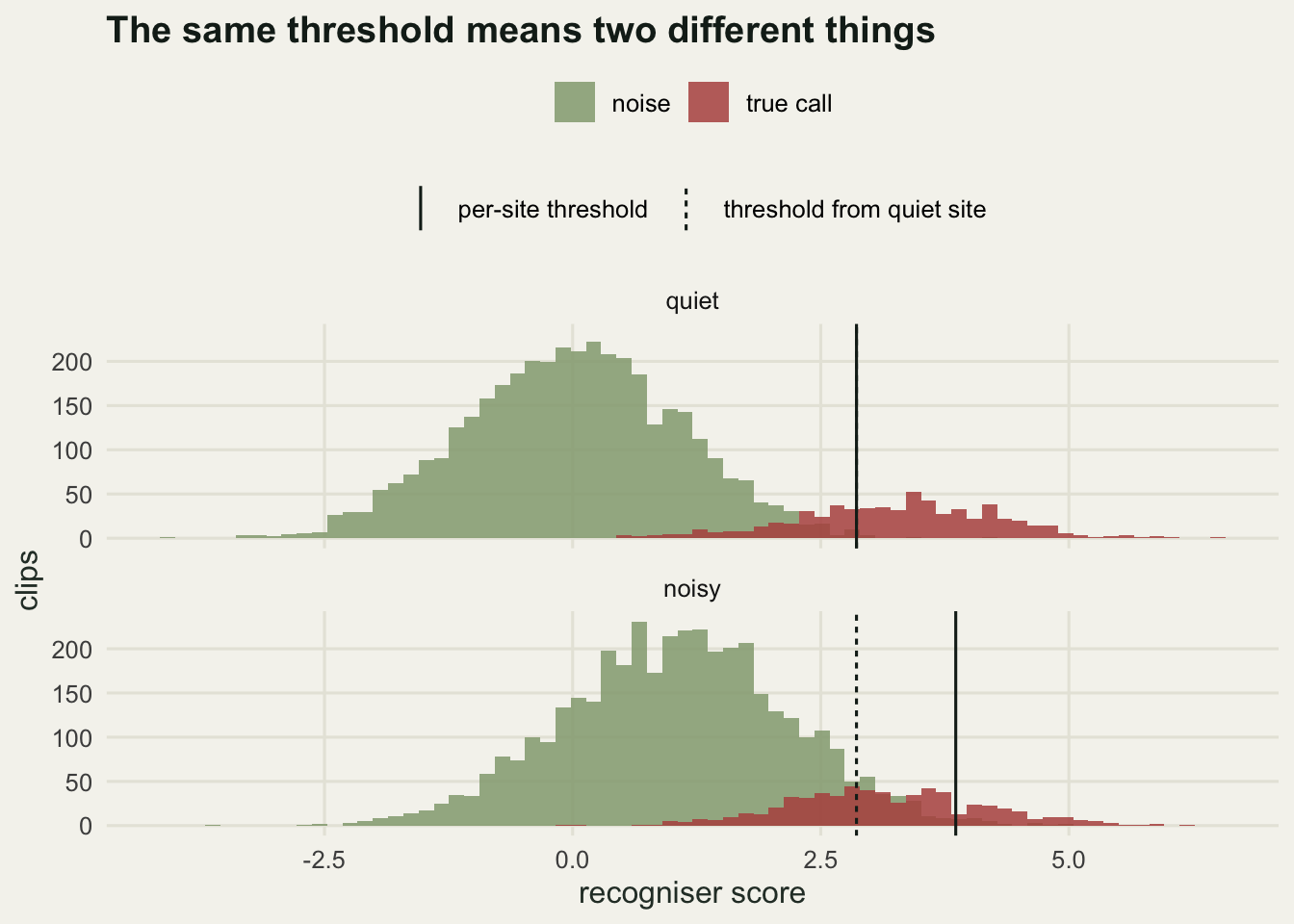
What does work is to stop comparing raw detection counts and compare a corrected index instead: detections multiplied by precision and divided by recall, with both factors estimated at each site from listened clips. Precision comes from listening to detections; recall needs a labelled set of true calls found by listening to raw audio, which is the expensive half.
n_val_clips <- 60L
n_val_calls <- 200L
n_draw <- 500L
print(c(listened_clips = n_val_clips, listened_calls = n_val_calls, draws = n_draw))
listened_clips listened_calls draws
60 200 500 corrected <- function(label, thr) {
v <- is_val & d_all$site == label
det <- which(v & d_all$score >= thr)
tru <- which(v & d_all$truth == 1L)
raw <- sum(u_use$score[u_use$site == label] >= thr) / hrs_use
vapply(seq_len(n_draw), function(b) {
p_hat <- mean(d_all$truth[sample(det, n_val_clips)])
r_hat <- mean(d_all$score[sample(tru, n_val_calls)] >= thr)
raw * p_hat / r_hat
}, numeric(1))
}
cq <- corrected("quiet", thr_q)
cn <- corrected("noisy", thr_q)
print(round(c(index_quiet = mean(cq), sd_quiet = sd(cq),
index_noisy = mean(cn), sd_noisy = sd(cn),
ratio = mean(cn / cq), sd_ratio = sd(cn / cq),
bias_corrected = mean(cn / cq) - truth_ratio), 4)) index_quiet sd_quiet index_noisy sd_noisy ratio
6.1018 0.2768 6.2628 0.5862 1.0286
sd_ratio bias_corrected
0.1087 0.0445 Across 500 draws of the validation sample, the corrected index averages 6.1018 calls per hour at the quiet site and 6.2628 at the noisy site, against realised truths of 6.5625 and 6.4583. The ratio is 1.0286 where the truth is 0.9841, so the error on this realisation is 0.0445 against 0.3888 for the raw comparison. That error comes from estimating the correction factors on the validation nights and applying them to different nights, with the same clips setting the threshold and the precision. Two uncertainties sit behind it. Redrawing the validation sample with the nights held fixed gives a standard deviation of 0.1087; the other one needs the whole survey generated again.
set.seed(5588)
n_survey <- 60L
n_draw_rep <- 200L
one_survey <- function() {
  dd <- rbind(sim_site("quiet", 0), sim_site("noisy", 1))
  vv <- dd$night <= n_val_nights
  uu <- dd[!vv, ]
  s_thr <- tune_thr(dd$score[vv & dd$site == "quiet"], dd$truth[vv & dd$site == "quiet"])
  draws <- function(label) {
    det_idx <- which(vv & dd$site == label & dd$score >= s_thr)
    tru <- which(vv & dd$site == label & dd$truth == 1L)
    raw <- sum(uu$score[uu$site == label] >= s_thr) / hrs_use
    vapply(seq_len(n_draw_rep), function(b)
      raw * mean(dd$truth[sample(det_idx, n_val_clips)]) /
        mean(dd$score[sample(tru, n_val_calls)] >= s_thr), numeric(1))
  }
  rr <- draws("noisy") / draws("quiet")
  c(err = mean(rr) - sum(uu$truth[uu$site == "noisy"]) / sum(uu$truth[uu$site == "quiet"]),
    sd_draw = sd(rr))
}
rep_out <- t(replicate(n_survey, one_survey()))
print(round(c(surveys = n_survey, mean_error = mean(rep_out[, "err"]),
              se_of_mean = sd(rep_out[, "err"]) / sqrt(n_survey),
              sd_error = sd(rep_out[, "err"]),
              min_error = min(rep_out[, "err"]), max_error = max(rep_out[, "err"]),
              mean_draw_sd = mean(rep_out[, "sd_draw"])), 4))
surveys mean_error se_of_mean sd_error min_error max_error
60.0000 0.0192 0.0212 0.1641 -0.3225 0.3854
mean_draw_sd
0.1202 Across sixty regenerated surveys the error runs from -0.3225 to 0.3854, with a standard deviation of 0.1641 around a mean of 0.0192, and that mean is smaller than its own standard error of 0.0212. The average spread within a single survey, 0.1202, is the smaller of the two. So the 0.0445 above is one draw from that distribution rather than a measurement of bias.
The correction is close to unbiased and not at all precise, and how much listening it takes to make it precise is the last check.
What a duty cycle costs depends on the question
Battery and card capacity force a duty cycle: record one minute in every six, or one in twelve. The received wisdom is that duty cycling costs little for presence and a lot for call rates. That is two claims about different estimators, and they can be measured on the same simulated nights.
A night is a fixed six-hour window. Three schedules are compared at each duty level: full coverage, a spread schedule that records one minute in every duty minutes, and a block schedule that records the same number of minutes in one contiguous stretch at the start. Spread and block cost the same battery; full coverage costs more, and is the reference the other two are measured against.
set.seed(77104)
span_min <- 360L
n_night <- 4000L
duty_set <- c(1L, 2L, 3L, 6L, 12L, 30L)
cue_per_min <- 0.075
bout_per_min <- 0.0125
print(c(span_minutes = span_min, simulated_nights = n_night,
        cues_per_minute = cue_per_min, bouts_per_minute = bout_per_min,
        mean_bout_size = 1 + bout_mu, duty_levels = length(duty_set)))
span_minutes simulated_nights cues_per_minute bouts_per_minute
3.60e+02 4.00e+03 7.50e-02 1.25e-02
mean_bout_size duty_levels
6.00e+00 6.00e+00 cues_poisson <- function() runif(rpois(1, cue_per_min * span_min), 0, span_min)
cues_bouts <- function() {
n_bouts <- rpois(1, bout_per_min * (span_min + bout_spread))
if (n_bouts == 0L) return(numeric(0))
onset <- runif(n_bouts, -bout_spread, span_min)
sizes <- 1L + rpois(n_bouts, bout_mu)
cues <- rep(onset, sizes) + runif(sum(sizes), 0, bout_spread)
cues[cues >= 0 & cues < span_min]
}
one_night <- function(gen) {
minute_of <- floor(gen())
vapply(duty_set, function(dd) {
c(sum(minute_of %% dd == 0L), sum(minute_of < span_min %/% dd))
}, numeric(2))
}
run_sched <- function(gen, label) {
arr <- replicate(n_night, one_night(gen))
out <- NULL
for (j in seq_along(duty_set)) {
recorded <- span_min %/% duty_set[j]
for (s in 1:2) {
cnt <- arr[s, j, ]
out <- rbind(out, data.frame(process = label,
schedule = c("spread", "block")[s],
duty = duty_set[j], recorded = recorded,
presence = mean(cnt > 0),
se_rate = sd(cnt / recorded)))
}
}
out
}
res_duty <- rbind(run_sched(cues_poisson, "Poisson"), run_sched(cues_bouts, "bouts"))
res_duty$fraction <- 1 / res_duty$duty
res_duty$se_ratio <- NA_real_
for (pr in unique(res_duty$process)) {
for (sch in unique(res_duty$schedule)) {
k <- res_duty$process == pr & res_duty$schedule == sch
res_duty$se_ratio[k] <- res_duty$se_rate[k] / res_duty$se_rate[k & res_duty$duty == 1L]
}
}
print(res_duty[res_duty$duty %in% c(1L, 6L), ], digits = 4) process schedule duty recorded presence se_rate fraction se_ratio
1 Poisson spread 1 360 1.0000 0.01433 1.0000 1.000
2 Poisson block 1 360 1.0000 0.01433 1.0000 1.000
7 Poisson spread 6 60 0.9910 0.03524 0.1667 2.460
8 Poisson block 6 60 0.9902 0.03498 0.1667 2.442
13 bouts spread 1 360 0.9915 0.03754 1.0000 1.000
14 bouts block 1 360 0.9915 0.03754 1.0000 1.000
19 bouts spread 6 60 0.8862 0.05845 0.1667 1.557
20 bouts block 6 60 0.5345 0.09208 0.1667 2.453pres_of <- function(pr, sch, dd) {
res_duty$presence[res_duty$process == pr & res_duty$schedule == sch & res_duty$duty == dd]
}
loss_pois <- pres_of("Poisson", "spread", 1L) - pres_of("Poisson", "spread", 6L)
loss_bout <- pres_of("bouts", "spread", 1L) - pres_of("bouts", "spread", 6L)
print(round(c(sqrt_six = sqrt(6), presence_loss_poisson = loss_pois,
presence_loss_bouts = loss_bout, loss_ratio = loss_bout / loss_pois,
presence_bouts_one_in_30 = pres_of("bouts", "spread", 30L)), 4)) sqrt_six presence_loss_poisson presence_loss_bouts
2.4495 0.0090 0.1053
loss_ratio presence_bouts_one_in_30
11.6944 0.3375 Take the one-in-six schedule first, on the Poisson process. Presence, meaning at least one detection all night, falls from 1.0000 under full coverage to 0.9910 under the spread duty cycle. The rate estimate is a different matter: its standard error rises by a factor of 2.460, which is the square root of six, 2.4495, to within simulation noise. So the received wisdom holds for a homogeneous process. Presence costs almost nothing and precision on the rate degrades exactly with the sampled fraction.
The bout process breaks the presence half of that. Under full coverage, presence is 0.9915; under the same one-in-six spread schedule it falls to 0.8862. The loss is 0.1053 against 0.0090 for the Poisson process with the same mean rate, worse by a factor of nearly twelve, and for the expected reason: the sampled minutes can miss whole bouts, and a clustered process spends most of its night silent. Push to one minute in thirty and presence for the bout process reaches 0.3375. A survey that concludes absence from a duty-cycled recorder is making a statement about bout structure that it has not measured.
The measurement contradicts the received wisdom in the other direction as well, and the contradiction is worth keeping. For the bout process the spread duty cycle inflates the rate standard error by only 1.557, not by 2.460. Spreading the recorded minutes across the night breaks up the within-bout correlation, so each sampled minute carries more independent information than a minute inside a contiguous block does. The block schedule, at identical battery cost, inflates it by 2.453 and drops presence to 0.5345. On a Poisson process the two schedules are interchangeable, 0.9910 against 0.9902. On a clustered process spreading wins on both counts, and it wins by more on presence than on rate.
keep_cols <- c("process", "schedule", "fraction")
duty_long <- rbind(
  data.frame(res_duty[keep_cols], quantity = "P(at least one detection)",
             value = res_duty$presence),
  data.frame(res_duty[keep_cols], quantity = "SE relative to full coverage",
             value = res_duty$se_ratio))
duty_long$schedule <- factor(duty_long$schedule, c("spread", "block"))

p_duty <- ggplot(duty_long, aes(fraction, value, colour = process, linetype = schedule)) +
  geom_line(linewidth = 0.7) +
  geom_point(size = 1.6) +
  facet_wrap(~ quantity, scales = "free_y") +
  scale_x_log10(labels = c("1/30", "1/12", "1/6", "1/3", "1"),
                breaks = c(1/30, 1/12, 1/6, 1/3, 1), minor_breaks = NULL) +
  scale_linetype_manual(values = c(spread = 1, block = 2)) +
  scale_colour_manual(values = c(Poisson = te_pal$sage, bouts = te_pal$forest)) +
  labs(title = "A duty cycle is cheap for presence only if calls are unclustered",
       x = "fraction of the night recorded", y = NULL, colour = NULL, linetype = NULL) +
  theme_te() + theme(legend.position = "top")
p_duty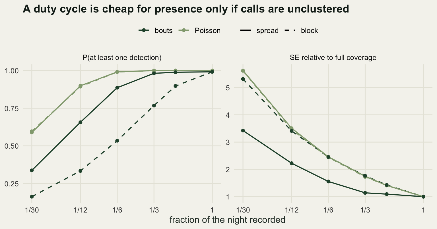
How many clips have to be listened to
The corrected index from the first post of this cluster multiplies a raw detection count by precision, and treats precision as known. It is not known; it is estimated by listening to a sample of detections and labelling them. That estimate has a standard error, and what happens to that error as a survey grows depends on how the listening is shared out. If one validation set is listened to for the whole survey, the error is common to every site: adding sites buys down the count sampling term and leaves the validation term exactly where it was. A fixed total listening budget split between the sites behaves the same way, because spreading the same clips over more sites leaves the averaged estimate as noisy as it was. What does buy the validation term down is a fixed number of clips at every site, which makes it shrink with the number of sites as well. The grid below is the common-validation case, and the clip counts in it are survey totals.
The standard error of an estimated false-trigger rate from a binomial sample of listened clips is the same number as the standard error of precision, because the two are complements. No design choice makes one of them cheaper than the other.
set.seed(9152)
prec_true <- 0.72
det_rate <- 6.25
n_site_grid <- c(10L, 30L, 100L)
clip_grid <- c(25L, 50L, 100L, 200L, 400L, 800L, 1600L)
n_sim <- 3000L
phi_carry <- round(vmr(clus_counts), 2)
print(c(precision = prec_true, false_trigger = 1 - prec_true,
        detections_per_hour = det_rate, recorder_hours = n_hours,
        dispersion = phi_carry, replicates = n_sim))
precision false_trigger detections_per_hour recorder_hours
0.72 0.28 6.25 12.00
dispersion replicates
6.83 3000.00 print(round(sqrt(prec_true * (1 - prec_true) / clip_grid), 4))[1] 0.0898 0.0635 0.0449 0.0317 0.0224 0.0159 0.0112Listening to 25 clips pins the false-trigger rate to a standard error of 0.0898; listening to 1600 pins it to 0.0112. Sixty-four times the effort for eight times the precision, which is the square-root law and cannot be improved by clever sampling.
Whether that matters depends on what it is being compared against. The regional mean of the corrected index across sites has a variance with two terms: count sampling, which carries the dispersion measured in the first check and shrinks with the number of sites, and the validation term, which does not shrink when one validation set serves the whole survey. Setting the two equal gives the number of clips at which the correction stops dominating. The simulation below draws site counts from a negative binomial matched to the measured dispersion and draws the precision estimate from a binomial, then compares the empirical standard deviation with the delta-method formula.
nb_size <- det_rate / (phi_carry - 1)
grd <- expand.grid(clips = clip_grid, sites = n_site_grid)
grd$var_count <- prec_true^2 * phi_carry * det_rate / (n_hours * grd$sites)
grd$var_clips <- det_rate^2 * prec_true * (1 - prec_true) / grd$clips
grd$se_total <- sqrt(grd$var_count + grd$var_clips)
grd$se_sim <- NA_real_
for (i in seq_len(nrow(grd))) {
  cm <- matrix(rnbinom(n_sim * grd$sites[i] * n_hours, size = nb_size, mu = det_rate),
               nrow = n_sim)
  p_hat <- rbinom(n_sim, grd$clips[i], prec_true) / grd$clips[i]
  grd$se_sim[i] <- sd(rowMeans(cm) * p_hat)
}
grd$se_count <- sqrt(grd$var_count)
grd$se_clips <- sqrt(grd$var_clips)
clip_star <- det_rate * (1 - prec_true) * n_hours * n_site_grid / (prec_true * phi_carry)
print(round(setNames(clip_star, paste0("sites_", n_site_grid)), 1))
sites_10 sites_30 sites_100
42.7 128.1 427.0 print(grd[grd$sites == 30L, c("clips", "sites", "se_count", "se_clips",
"se_total", "se_sim")], digits = 4) clips sites se_count se_clips se_total se_sim
8 25 30 0.2479 0.56125 0.6136 0.6145
9 50 30 0.2479 0.39686 0.4679 0.4829
10 100 30 0.2479 0.28062 0.3745 0.3761
11 200 30 0.2479 0.19843 0.3176 0.3204
12 400 30 0.2479 0.14031 0.2849 0.2866
13 800 30 0.2479 0.09922 0.2670 0.2681
14 1600 30 0.2479 0.07016 0.2577 0.2624The crossover sits at 42.7 listened clips in total for a ten-site survey, 128.1 for thirty sites and 427.0 for a hundred sites. Below those numbers the uncertainty in the corrected index is mostly uncertainty about the recogniser; above them it is mostly uncertainty about the animals. The scaling is linear in the number of sites: a survey that doubles its sites has to double its listening just to stay in the same place.
For thirty sites the arithmetic is stark. At 100 listened clips the total standard error is 0.3745 calls per hour; at 1600 clips it is 0.2577, and the floor set by count sampling alone is 0.2479. Sixteen times the listening effort removes about a third of the total uncertainty, and everything below 0.2479 is unreachable without more recorders. The simulated standard deviations track the delta-method formula closely, so the decomposition can be used for design work.
val_cols <- c("clips", "sites")
val_long <- rbind(
  data.frame(grd[val_cols], term = "count sampling", se = grd$se_count),
  data.frame(grd[val_cols], term = "validation set", se = grd$se_clips),
  data.frame(grd[val_cols], term = "total", se = grd$se_total))
val_long$sites <- factor(paste(val_long$sites, "sites"),
                         paste(n_site_grid, "sites"))
star_dat <- data.frame(sites = factor(paste(n_site_grid, "sites"),
                                      paste(n_site_grid, "sites")),
                       xint = clip_star)

p_val <- ggplot(val_long, aes(clips, se, colour = term)) +
  geom_vline(data = star_dat, aes(xintercept = xint), linetype = 2,
             colour = te_pal$ink) +
  geom_line(linewidth = 0.7) +
  geom_point(size = 1.5) +
  facet_wrap(~ sites) +
  scale_x_log10() +
  scale_y_log10() +
  scale_colour_manual(values = c("count sampling" = te_pal$sage,
                                 "validation set" = te_pal$clay,
                                 total = te_pal$forest)) +
  labs(title = "Where listening stops being the limiting cost",
       x = "listened validation clips (survey total)", y = "SE of the mean index",
       colour = NULL) +
  theme_te() + theme(legend.position = "top")
p_val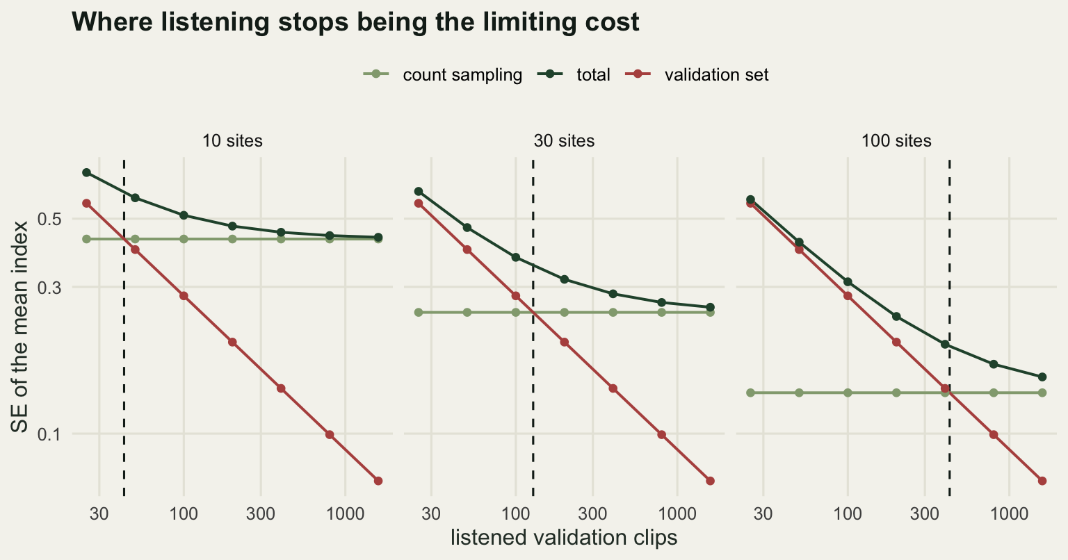
What none of these checks can catch
Every check above tests the machinery against itself. The simulator knows which cues are calls and which are noise, so the diagnostics are asking whether the estimator recovers a truth that was written into the data. That is a real question and the answers are useful, but it is a narrower question than the one a monitoring study is asked.
All four checks assume the labelled validation clips are correctly labelled. If a listener scores a marginal clip as the target species when it is not, precision is biased upward, the corrected index is biased upward, and no amount of extra listening finds the error: the validation term shrinks toward the wrong number. The gate on that is a second listener and a measured agreement rate, not a bigger sample.
All four also assume the target species is the only source of that call type. It usually is not. A congener with a similar call, or a mimic, produces detections that arrive in bouts, that score highly, that respond to the recogniser threshold the same way, and that are consistent between sites and nights. Such a signal passes the overdispersion check, passes the threshold-transfer check, passes the duty-cycle arithmetic and passes the validation-size calculation, because it is a real acoustic signal being detected correctly by a recogniser that was asked the wrong question. Every diagnostic in this post would call that survey clean. Only listening to the audio, or looking at a spectrogram, or an independent survey by another method, catches it.
There is no statistical repair for a species identification that is wrong at the source. The honest reporting is to state which clips were verified by ear, by whom, and how many, and to treat the recogniser output as an index of an acoustic signal rather than as a count of a species until that verification exists.
Where to go next
This closes the acoustic cluster. The first post left a corrected index that assumed a known false-trigger rate, and the fourth check above says how many clips it takes to earn that assumption. The second post left a threshold chosen against precision, and the second check says that the threshold is a property of the site rather than of the recogniser. The third post left a call rate on the way to density, and the first and third checks say what the interval around that rate should be and what a duty cycle does to it.
The same false-positive logic runs through eDNA surveys, where a contaminated PCR replicate plays the part of a high-scoring noise clip, and through occupancy models with false positives, where the mixture is written into the likelihood rather than corrected afterwards. The estimator differs; the accounting does not.
References
Shonfield J, Bayne EM 2017 Avian Conservation and Ecology 12(1):14 (10.5751/ACE-00974-120114)
Sugai LSM, Silva TSF, Ribeiro JW, Llusia D 2019 BioScience 69(1):15-25 (10.1093/biosci/biy147)
Miller DA, Nichols JD, McClintock BT, Grant EHC, Bailey LL, Weir LA 2011 Ecology 92(7):1422-1428 (10.1890/10-1396.1)
Royle JA, Link WA 2006 Ecology 87(4):835-841 (10.1890/0012-9658(2006)87[835:GSOMAF]2.0.CO;2)
Bolker BM, Brooks ME, Clark CJ, Geange SW, Poulsen JR, Stevens MHH, White JSS 2009 Trends in Ecology and Evolution 24(3):127-135 (10.1016/j.tree.2008.10.008)