library(ggplot2)

te_pal <- list(forest = "#275139", green = "#2f8f63", sage = "#93a87f",
               clay = "#b5534e", gold = "#cda23f", line = "#dad9ca",
               ink = "#16241d", paper = "#f5f4ee")

theme_te <- function() {
  theme_minimal(base_size = 12) +
    theme(panel.grid.minor = element_blank(),
          panel.grid.major = element_line(colour = "#e7e6dc"),
          plot.background = element_rect(fill = "#f5f4ee", colour = NA),
          panel.background = element_rect(fill = "#f5f4ee", colour = NA),
          plot.title = element_text(face = "bold", colour = te_pal$ink),
          axis.title = element_text(colour = "#2c3a31"))
}Call rates and density from acoustic surveys
R
bioacoustics
acoustic monitoring
abundance
imperfect detection
ecology tutorial
ggplot2
Cue counting in base R: turn acoustic detection rates into density, and measure which part of the variance dominates and which bias passes through undamped.
A recorder array gives you cues, not animals. A detector run over a season of audio returns a count of song events, echolocation clicks or whistles, and the count is a product of three things you did not measure separately: how many animals were within earshot, how often each one called, and how far the microphone could hear. Cue counting is the estimator that pulls those apart, and it is the standard route from an automated detection pipeline to a density in animals per hectare.
The arithmetic is short. Density equals the number of detected cues, divided by the survey time, divided by the mean number of cues an animal produces per unit time, divided by the effective area over which a cue can be detected. Three divisions, three estimated inputs. The interesting part is not the point estimate; it is that the three inputs are measured with wildly different precision, and that an error in one of them behaves completely differently from an error in another. This tutorial builds each component by hand in base R, checks the estimator against a simulated population of known density, and then spends most of its time measuring where the uncertainty and the bias come from.
If you have not yet turned detector output into a defensible count, start with automated acoustic detections as data; everything below assumes you already have a cue count you trust.
Cue counting, and the three things it needs
Write the estimator out. With n cues detected across K recorder stations each running for T hours, a mean cue production rate r per animal per hour, and an effective detection area nu, the density estimate is n / (K * T * r * nu). Every term is an estimate except the recording effort.
The effective detection area is the one piece that is pure geometry plus a detection function. If a cue at distance x is detected with probability g(x), then integrating 2 * pi * x * g(x) over distance gives the area of the disc that would yield the same number of detections if detection inside it were perfect and outside it were zero. For a half-normal g(x) = exp(-x^2 / (2 * sigma^2)) the integral has a closed form, 2 * pi * sigma^2, and the effective radius is sqrt(2) * sigma. Start with the design constants.
dens_true     <- 0.8    # animals per hectare
sigma_true    <- 50     # half-normal scale, metres
cue_rate_true <- 12     # cues per animal per hour
cue_cv_ind    <- 0.45   # between-individual CV in cue rate
n_stations    <- 20
hours_per_stn <- 30
n_focal       <- 8      # focal animals used for the cue rate
focal_hours   <- 1      # hours each focal animal is followed
n_localised   <- 120    # detected cues with a measured distance
rmax          <- 400    # simulation radius, metres
n_rep         <- 3000   # simulated surveys

design <- data.frame(
  quantity = c("true density (per ha)", "half-normal sigma (m)",
               "cue rate (per animal per hour)", "between-animal CV in cue rate",
               "recorder stations", "hours per station", "focal animals",
               "hours per focal animal", "localised cues", "simulated surveys"),
  value = c(dens_true, sigma_true, cue_rate_true, cue_cv_ind, n_stations,
            hours_per_stn, n_focal, focal_hours, n_localised, n_rep))
print(design)
quantity value
1 true density (per ha) 0.80
2 half-normal sigma (m) 50.00
3 cue rate (per animal per hour) 12.00
4 between-animal CV in cue rate 0.45
5 recorder stations 20.00
6 hours per station 30.00
7 focal animals 8.00
8 hours per focal animal 1.00
9 localised cues 120.00
10 simulated surveys 3000.00Now the effective area, three ways: the closed form, a numerical integral, and a simulation that throws candidate cues uniformly over a disc and keeps the ones the detection function accepts.
set.seed(20260814)
g_hn <- function(x, sig) exp(-x^2 / (2 * sig^2))

nu_closed  <- 2 * pi * sigma_true^2
nu_numeric <- integrate(function(x) 2 * pi * x * g_hn(x, sigma_true), 0, Inf)$value

n_cand <- 400000
xcand  <- rmax * sqrt(runif(n_cand))
hit    <- runif(n_cand) < g_hn(xcand, sigma_true)
nu_mc  <- mean(hit) * pi * rmax^2

cat("candidate cues thrown:", format(n_cand, scientific = FALSE), "\n")
candidate cues thrown: 400000 cat("effective area, closed form (m2):", round(nu_closed, 1), "\n")effective area, closed form (m2): 15708 cat("effective area, numerical integral (m2):", round(nu_numeric, 1), "\n")effective area, numerical integral (m2): 15708 cat("effective area, simulation (m2):", round(nu_mc, 1), "\n")effective area, simulation (m2): 15563.5 cat("effective radius (m):", round(sqrt(2) * sigma_true, 2), "\n")effective radius (m): 70.71 cat("effective area (ha):", round(nu_closed / 10000, 4), "\n")effective area (ha): 1.5708 cat("share of the effective area within 20 m:",
round(1 - exp(-20^2 / (2 * sigma_true^2)), 4), "\n")share of the effective area within 20 m: 0.0769 cat("share of the effective area within the effective radius:",
round(1 - exp(-1), 4), "\n")share of the effective area within the effective radius: 0.6321 The three agree. The hazard-rate form is the usual alternative: g(x) = 1 - exp(-(x / sigma)^(-b)), which holds a flat shoulder near the recorder and then falls away sharply. Its effective area is pi * sigma^2 * gamma(1 - 2 / b), defined for b > 2. Pick the hazard-rate scale so that the two functions have exactly the same effective area; that way the only difference between them later is shape.
b_hr   <- 6
g_hr   <- function(x, sig, bb) 1 - exp(-(x / sig)^(-bb))
sig_hr <- sqrt(nu_closed / (pi * gamma(1 - 2 / b_hr)))

nu_hr_closed  <- pi * sig_hr^2 * gamma(1 - 2 / b_hr)
nu_hr_numeric <- integrate(function(x) 2 * pi * x * g_hr(x, sig_hr, b_hr), 0, Inf)$value

cat("hazard-rate shape b:", b_hr, "\n")
hazard-rate shape b: 6 cat("hazard-rate scale matched on effective area (m):", round(sig_hr, 2), "\n")hazard-rate scale matched on effective area (m): 60.77 cat("hazard-rate effective area, closed form (m2):", round(nu_hr_closed, 1), "\n")hazard-rate effective area, closed form (m2): 15708 cat("hazard-rate effective area, numerical (m2):", round(nu_hr_numeric, 1), "\n")hazard-rate effective area, numerical (m2): 15708 xg <- seq(0, 220, by = 0.5)
fig1 <- rbind(
data.frame(x = xg, form = "half-normal", panel = "detection probability g(x)",
y = g_hn(xg, sigma_true)),
data.frame(x = xg, form = "hazard-rate", panel = "detection probability g(x)",
y = g_hr(xg, sig_hr, b_hr)),
data.frame(x = xg, form = "half-normal", panel = "integrand 2 pi x g(x)",
y = 2 * pi * xg * g_hn(xg, sigma_true)),
data.frame(x = xg, form = "hazard-rate", panel = "integrand 2 pi x g(x)",
y = 2 * pi * xg * g_hr(xg, sig_hr, b_hr)))
p1 <- ggplot(fig1, aes(x, y, colour = form)) +
geom_line(linewidth = 0.9) +
facet_wrap(~panel, scales = "free_y") +
scale_colour_manual(values = c("half-normal" = te_pal$green,
"hazard-rate" = te_pal$clay)) +
labs(x = "distance from recorder (metres)", y = NULL,
colour = NULL, title = "Same effective area, different shape") +
theme_te() + theme(legend.position = "top")
print(p1)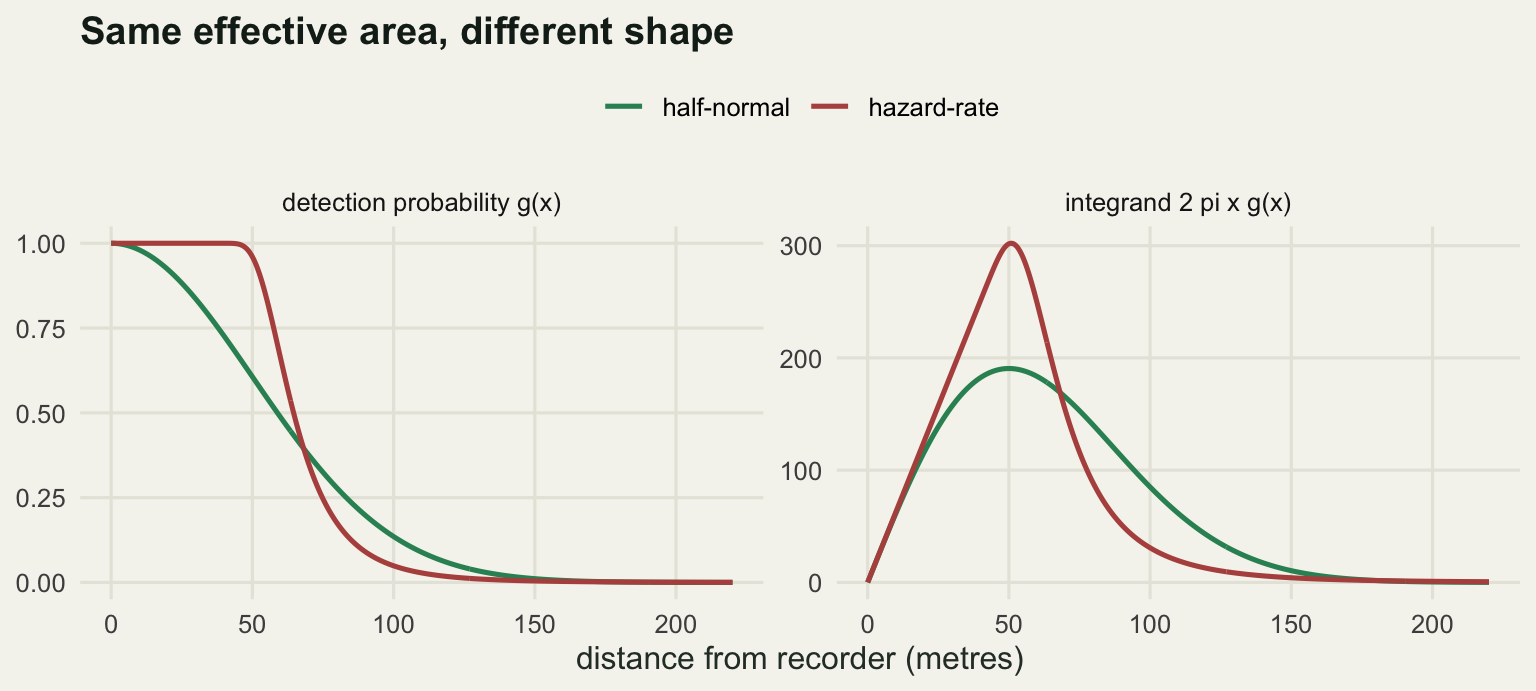
The right panel is the part that gets forgotten. Detection probability is highest at the recorder, but the area contribution peaks well out from it, because there is more ground at larger distances. Only 7.69 per cent of the half-normal effective area comes from the first twenty metres, and 63.21 per cent of it from inside the effective radius; the rest is contributed by cues that are individually unlikely to be detected but numerous.
What the estimator recovers
The simulator places animals at the true density in a disc around each station, gives each animal its own cue rate drawn from a gamma with the specified between-individual variation, and thins its cues by the detection function. An animal at distance x contributes a Poisson number of detected cues with mean rate * hours * g(x), so the whole survey can be generated without ever enumerating an undetected cue.
The three inputs then come from three separate pieces of data, as they do in the field. The count comes from the stations. The detection function is fitted to a subsample of cues whose distance was measured, by localisation or by a calibrated array; for a half-normal, detected distances follow a Rayleigh distribution with scale sigma, so the maximum likelihood estimate is sqrt(mean(x^2) / 2). The cue rate comes from following a handful of focal animals for a fixed time.
set.seed(20260814)

sim_survey <- function(ns, hrs, nf, nl) {
  lam_a  <- dens_true * pi * rmax^2 / 10000          # expected animals per station
  n_anim <- rpois(1, ns * lam_a)
  stn    <- sample.int(ns, n_anim, replace = TRUE)
  xa     <- rmax * sqrt(runif(n_anim))
  ind_r  <- rgamma(n_anim, shape = 1 / cue_cv_ind^2, scale = cue_rate_true * cue_cv_ind^2)
  cues   <- rpois(n_anim, ind_r * hrs * g_hn(xa, sigma_true))
  per    <- as.numeric(tapply(cues, factor(stn, levels = seq_len(ns)), sum))
  per[is.na(per)] <- 0

  xl     <- sigma_true * sqrt(-2 * log(runif(nl)))   # localised detected distances
  sig_h  <- sqrt(mean(xl^2) / 2)
  nu_h   <- 2 * pi * sig_h^2 / 10000                 # hectares

  lam_f  <- rgamma(nf, shape = 1 / cue_cv_ind^2, scale = cue_rate_true * cue_cv_ind^2)
  r_h    <- mean(rpois(nf, lam_f * focal_hours)) / focal_hours

  c(cues = sum(per), encounter = sum(per) / (ns * hrs), nu_hat = nu_h,
    r_hat = r_h, dhat = sum(per) / (ns * hrs * r_h * nu_h))
}

one <- sim_survey(n_stations, hours_per_stn, n_focal, n_localised)
print(round(one, 4))
cues encounter nu_hat r_hat dhat
6847.0000 11.4117 1.5048 13.0000 0.5833 One survey is one draw. Repeat it.
set.seed(101)
sims <- t(replicate(n_rep, sim_survey(n_stations, hours_per_stn,
                                      n_focal, n_localised)))

d_mean <- mean(sims[, "dhat"])
d_med  <- median(sims[, "dhat"])
d_cv   <- sd(sims[, "dhat"]) / d_mean

cat("true density (per ha):", dens_true, "\n")
true density (per ha): 0.8 cat("mean estimate:", round(d_mean, 4), "\n")mean estimate: 0.8387 cat("median estimate:", round(d_med, 4), "\n")median estimate: 0.8023 cat("relative bias of the mean:", round(d_mean / dens_true - 1, 4), "\n")relative bias of the mean: 0.0484 cat("relative bias of the median:", round(d_med / dens_true - 1, 4), "\n")relative bias of the median: 0.0029 cat("CV of the estimate:", round(d_cv, 4), "\n")CV of the estimate: 0.2754 cat("central 90 per cent of estimates:",
round(quantile(sims[, "dhat"], c(0.05, 0.95)), 4), "\n")central 90 per cent of estimates: 0.5317 1.285 p2 <- ggplot(data.frame(dhat = sims[, "dhat"]), aes(dhat)) +
geom_histogram(bins = 60, fill = te_pal$sage, colour = NA) +
geom_vline(xintercept = dens_true, colour = te_pal$forest, linewidth = 1) +
geom_vline(xintercept = d_mean, colour = te_pal$clay,
linewidth = 0.9, linetype = "dashed") +
labs(x = "estimated density (animals per hectare)",
y = "simulated surveys", title = "Recovery of a known density") +
theme_te()
print(p2)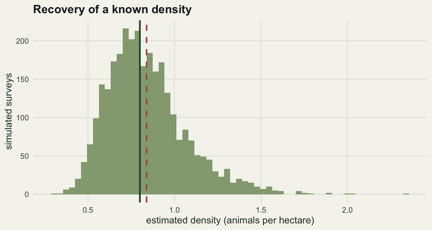
The median sits close to the truth and the mean sits above it. That upward pull is not a coding slip: the estimator divides by two estimated quantities, and the expectation of a reciprocal exceeds the reciprocal of the expectation. The size of the pull is set largely by the small focal sample, and it is the first hint of where this estimator keeps its problems.
Where the uncertainty actually lives, and what more effort buys
The delta method says that for a product or quotient of independent terms, squared coefficients of variation add. So the squared CV of the density estimate is the sum of the squared CVs of the encounter rate, the effective area and the cue rate. Each of the three CVs can be read straight off the simulation, and their sum can be checked against the CV of the density estimates themselves.
cv_er <- sd(sims[, "encounter"]) / mean(sims[, "encounter"])
cv_nu <- sd(sims[, "nu_hat"])    / mean(sims[, "nu_hat"])
cv_r  <- sd(sims[, "r_hat"])     / mean(sims[, "r_hat"])
cv_delta <- sqrt(cv_er^2 + cv_nu^2 + cv_r^2)

decomp <- data.frame(
  component = c("encounter rate", "effective area", "cue rate"),
  cv = c(cv_er, cv_nu, cv_r),
  share = c(cv_er, cv_nu, cv_r)^2 / cv_delta^2)
print(round(decomp[, 2:3], 4))
cv share
1 0.1558 0.3554
2 0.0902 0.1190
3 0.1895 0.5257print(decomp$component)[1] "encounter rate" "effective area" "cue rate" cat("delta-method total CV:", round(cv_delta, 4), "\n")delta-method total CV: 0.2614 cat("simulated total CV:", round(d_cv, 4), "\n")simulated total CV: 0.2754 cat("effective-area CV, analytic 1/sqrt(localised cues):",
round(1 / sqrt(n_localised), 4), "\n")effective-area CV, analytic 1/sqrt(localised cues): 0.0913 cat("recorder-hours in the baseline design:", n_stations * hours_per_stn, "\n")recorder-hours in the baseline design: 600 The decomposition closes to within a few per cent: the delta-method total is 0.2614 and the simulated total 0.2754, the simulated value running higher because the delta method is a first-order approximation and ignores the reciprocal bias that already shifted the mean. The shares are the point of the post. The cue rate, estimated from eight animals followed for an hour each, carries a CV of 0.1895 and accounts for 52.57 per cent of the variance of the density estimate. The encounter rate, built from 20 stations and 600 recorder-hours, contributes 35.54 per cent, and the fitted detection function only 11.9 per cent. The effective-area CV also has a closed form here: for a half-normal fitted to Rayleigh distances it is one over the square root of the number of localised cues, 0.0913 against a simulated 0.0902.
d3 <- decomp
d3$component <- factor(d3$component, levels = d3$component[order(d3$share)])
p3 <- ggplot(d3, aes(component, share, fill = component)) +
  geom_col(width = 0.62) +
  geom_text(aes(label = sprintf("%.1f%%", 100 * share)), hjust = -0.15, size = 4) +
  coord_flip(clip = "off") +
  scale_y_continuous(limits = c(0, 0.65)) +
  scale_fill_manual(values = c("cue rate" = te_pal$clay,
                               "encounter rate" = te_pal$green,
                               "effective area" = te_pal$sage)) +
  labs(x = NULL, y = "share of the variance of the density estimate",
       fill = NULL, title = "The multiplier carries the variance") +
  theme_te() + theme(legend.position = "none")
print(p3)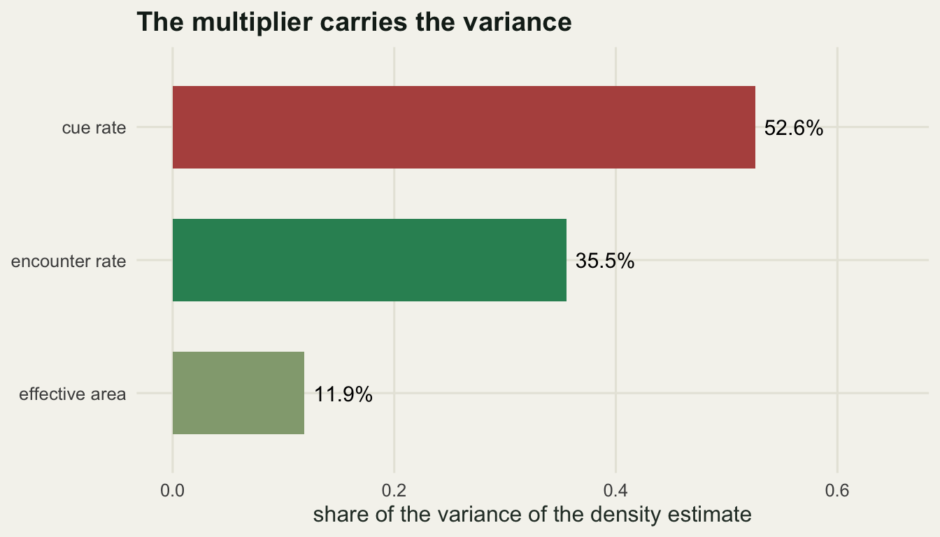
That has an immediate consequence for survey design. The encounter rate and the effective area both improve with recorder effort; the cue rate does not, because it is measured elsewhere. Run the whole simulation under six effort settings and compare.
set.seed(777)
effort_cv <- function(ns, hrs, nf, nl, reps = 5000) {
  m <- t(replicate(reps, sim_survey(ns, hrs, nf, nl)))
  c(cv_er = sd(m[, "encounter"]) / mean(m[, "encounter"]),
    cv_nu = sd(m[, "nu_hat"]) / mean(m[, "nu_hat"]),
    cv_r  = sd(m[, "r_hat"]) / mean(m[, "r_hat"]),
    cv_total = sd(m[, "dhat"]) / mean(m[, "dhat"]))
}

scen <- rbind(
  base = effort_cv(20, 30, 8, 120),
  double_stations = effort_cv(40, 30, 8, 240),
  double_hours = effort_cv(20, 60, 8, 240),
  double_focal = effort_cv(20, 30, 16, 120),
  double_both = effort_cv(40, 30, 16, 240),
  ten_times_stations = effort_cv(200, 30, 8, 1200, reps = 2500))
print(round(scen, 4))
cv_er cv_nu cv_r cv_total
base 0.1554 0.0911 0.1895 0.2717
double_stations 0.1092 0.0653 0.1856 0.2321
double_hours 0.1554 0.0646 0.1919 0.2614
double_focal 0.1562 0.0907 0.1343 0.2322
double_both 0.1094 0.0641 0.1326 0.1889
ten_times_stations 0.0494 0.0293 0.1889 0.2077cat("floor set by the cue rate (CV of the cue rate alone):", round(cv_r, 4), "\n")floor set by the cue rate (CV of the cue rate alone): 0.1895 cat("recorder-hours at ten times the array:", 200 * hours_per_stn, "\n")recorder-hours at ten times the array: 6000 Doubling the number of stations, and with them the number of localised cues, moves the total CV from 0.2717 to 0.2321. Doubling the focal sample from eight animals to sixteen, which costs two more mornings of fieldwork rather than twenty more recorders and their batteries, lands on 0.2322: the same precision, for a small fraction of the money. Doing both gets to 0.1889. And ten times the recorder effort, 200 stations and 6000 recorder-hours, still leaves a CV of 0.2077 against a floor of 0.1895, because the cue rate is untouched by any of it.
The double_hours row is the one that surprised me. Running the same 20 stations for 60 hours instead of 30 moves the total CV only from 0.2717 to 0.2614, even though it doubles the cue count, and all of that small gain comes from the extra localised distances: the encounter rate CV sits at 0.1554 in both rows, unchanged to four decimals. The same extra recorder-hours spent instead on twenty more stations give 0.2321. What a station records depends on how many animals happen to hold territories near it, and more hours at the same station cannot resample that. Extra recorder time buys precision on the wrong quantity; extra stations buy it on the right one, and even they run into the cue rate.
Cue rate is not a constant
Everything so far treated the cue rate as a fixed population property estimated with error. It is not fixed. Song output has a strong diel cycle, and the rate you measure depends entirely on when you measured it. Build a diel curve with a dawn peak and a smaller evening rise, scaled so that the daily mean is exactly the cue rate used throughout.
diel_shape <- function(h) 1 + 3.4 * exp(-(h - 5)^2 / (2 * 1.2^2)) +
                              1.1 * exp(-(h - 19)^2 / (2 * 1.0^2))
hgrid <- seq(0, 24, length.out = 20001)
scal  <- cue_rate_true / mean(diel_shape(hgrid))
cue_at <- function(h) scal * diel_shape(h)

r_daily <- mean(cue_at(hgrid))
dawn    <- hgrid >= 4 & hgrid <= 6.5
r_dawn  <- mean(cue_at(hgrid[dawn]))
peak_ratio <- r_dawn / r_daily

cat("daily mean cue rate:", round(r_daily, 3), "\n")
daily mean cue rate: 12 cat("mean cue rate in the dawn window 04:00 to 06:30:", round(r_dawn, 3), "\n")mean cue rate in the dawn window 04:00 to 06:30: 29.834 cat("ratio of dawn rate to daily mean:", round(peak_ratio, 3), "\n")ratio of dawn rate to daily mean: 2.486 Now run two schedules. In the first the recorders run around the clock, so the cues accumulate at the daily mean rate, but the cue rate multiplier was measured during the dawn chorus because that is when the focal follows were done. In the second the recorders run only in the dawn window, so the cues accumulate at the peak rate, but the multiplier used is a published daily mean.
set.seed(31)
nu_ha  <- nu_closed / 10000
days   <- 20
hrs_all  <- 24 * days * n_stations
hrs_dawn <- 2.5 * days * n_stations

n_all  <- rpois(1, dens_true * nu_ha * r_daily * hrs_all)
n_dawn <- rpois(1, dens_true * nu_ha * r_dawn * hrs_dawn)

d_all_right <- n_all / (hrs_all * r_daily * nu_ha)
d_all_wrong <- n_all / (hrs_all * r_dawn  * nu_ha)
d_dawn_wrong <- n_dawn / (hrs_dawn * r_daily * nu_ha)

cat("all-day recording, correct daily rate:", round(d_all_right, 4), "\n")
all-day recording, correct daily rate: 0.8001 cat("all-day recording, dawn rate used:", round(d_all_wrong, 4),
" ratio to truth:", round(d_all_wrong / dens_true, 3), "\n")all-day recording, dawn rate used: 0.3218 ratio to truth: 0.402 cat("dawn-only recording, daily rate used:", round(d_dawn_wrong, 4),
" ratio to truth:", round(d_dawn_wrong / dens_true, 3), "\n")dawn-only recording, daily rate used: 1.987 ratio to truth: 2.484 cat("1 / peak ratio:", round(1 / peak_ratio, 3), "\n")1 / peak ratio: 0.402 p4 <- ggplot(data.frame(h = hgrid, y = cue_at(hgrid)), aes(h, y)) +
annotate("rect", xmin = 4, xmax = 6.5, ymin = 0, ymax = Inf,
fill = te_pal$gold, alpha = 0.22) +
geom_line(colour = te_pal$forest, linewidth = 0.9) +
geom_hline(yintercept = r_daily, colour = te_pal$clay,
linewidth = 0.8, linetype = "dashed") +
scale_x_continuous(breaks = seq(0, 24, by = 4)) +
labs(x = "hour of day", y = "cues per animal per hour",
colour = NULL, title = "The multiplier depends on when you measured it") +
theme_te()
print(p4)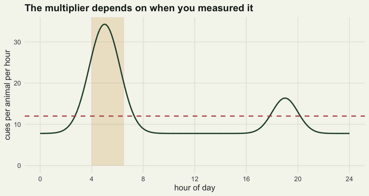
The two ratios are the whole story. The dawn rate is 2.486 times the daily mean, and the all-day survey that uses it comes out at 0.402 of the true density: the same number, upside down. The dawn-only survey that uses the daily mean overestimates by the same factor, 2.484. A cue rate error is a pure multiplicative bias on the density; it is transmitted one for one, with nothing in the acoustic data to absorb it or to flag it.
What a wrong detection function costs by comparison
I expected the detection function to be the safer of the two, on the grounds that the detection function is fitted to data from the survey itself and so partly self-corrects. Test it. Generate detected distances from the hazard-rate function, which has exactly the same effective area as the half-normal, and fit a half-normal to them anyway.
set.seed(9090)
xgrid_hr <- seq(0, 4000, by = 0.25)
dens_hr  <- 2 * pi * xgrid_hr * g_hr(xgrid_hr, sig_hr, b_hr)
cdf_hr   <- c(0, cumsum((dens_hr[-1] + dens_hr[-length(dens_hr)]) / 2 * 0.25))
cat("mass on the sampling grid vs closed form (m2):",
    round(max(cdf_hr), 1), round(nu_hr_closed, 1), "\n")
mass on the sampling grid vs closed form (m2): 15707.9 15708 cdf_hr <- cdf_hr / max(cdf_hr)
draw_hr <- function(n) approx(cdf_hr, xgrid_hr, runif(n))$y
ex2 <- integrate(function(x) 2 * pi * x^3 * g_hr(x, sig_hr, b_hr),
0, 4000)$value / nu_hr_closed
sig_fit <- sqrt(ex2 / 2)
nu_fit <- 2 * pi * sig_fit^2
nu_fit_mc <- pi * mean(draw_hr(200000)^2)
cat("true effective area (hazard-rate, m2):", round(nu_hr_closed, 1), "\n")true effective area (hazard-rate, m2): 15708 cat("half-normal scale the fit converges to (m):", round(sig_fit, 2), "\n")half-normal scale the fit converges to (m): 42.73 cat("fitted effective area (m2):", round(nu_fit, 1),
" from 200000 simulated distances:", round(nu_fit_mc, 1), "\n")fitted effective area (m2): 11472.7 from 200000 simulated distances: 11484.5 cat("effective area ratio, fitted over true:", round(nu_fit / nu_hr_closed, 4), "\n")effective area ratio, fitted over true: 0.7304 cat("effective area underestimated by:", round(1 - nu_fit / nu_hr_closed, 3), "\n")effective area underestimated by: 0.27 cat("density inflated by a factor of:", round(nu_hr_closed / nu_fit, 4), "\n")density inflated by a factor of: 1.3692 cat("resulting bias in density:", round(nu_hr_closed / nu_fit - 1, 4), "\n")resulting bias in density: 0.3692 cat("bias if the hazard-rate scale were plugged into the half-normal formula:",
round(2 * pi * sig_hr^2 / nu_hr_closed - 1, 4), "\n")bias if the hazard-rate scale were plugged into the half-normal formula: 0.477 bias120 <- replicate(2000, nu_hr_closed / (pi * mean(draw_hr(n_localised)^2)) - 1)
cat("density bias with only 120 localised distances, median:",
round(median(bias120), 4), " 5th and 95th percentile:",
round(quantile(bias120, c(0.05, 0.95)), 4), "\n")density bias with only 120 localised distances, median: 0.4165 5th and 95th percentile: 0.0764 0.697 The measurement contradicts what I expected, so the claim has to give way. Fitting the wrong functional form underestimates the effective area by 27 per cent and therefore inflates density by 36.9 per cent. That is not a rounding error, and it is far more than “partly self-corrects” would suggest. There is real absorption: the fitted scale settles at 42.73 metres rather than the hazard-rate scale of 60.77, and plugging the latter into the half-normal formula would have overstated the area by 47.7 per cent. So the fit removes a little under half the parameter mismatch in area terms, and it still leaves a 36.9 per cent bias in density, in the opposite direction from the naive plug-in. With a realistic sample of 120 localised distances the bias is not even stable: its median across simulated surveys is 0.4165 with a 5th to 95th percentile spread from 0.0764 to 0.697, because the hazard-rate tail makes the mean of squared distances a badly behaved statistic.
So the honest ranking, on these two examples, is that the cue rate error is the larger one: a factor of 2.486 against a factor of 1.369. But they are the same order, not different orders, and anyone who treats the detection function as the safe component because it was fitted to data is wrong. What separates the two is not size, it is detectability. The distance data carry information about the shape of the detection function, so a wrong form leaves a trace in the residuals.
set.seed(5150)
gof_p <- function(xx) {
  sg  <- sqrt(mean(xx^2) / 2)
  brk <- c(0, sg * sqrt(-2 * log(1 - seq(0.125, 0.875, by = 0.125))), Inf)
  obs <- as.numeric(table(cut(xx, brk, include.lowest = TRUE)))
  expct <- rep(length(xx) / 8, 8)
  pchisq(sum((obs - expct)^2 / expct), df = 6, lower.tail = FALSE)
}

n_gof <- 1000
p_wrong <- replicate(n_gof, gof_p(draw_hr(n_localised)))
p_right <- replicate(n_gof, gof_p(sigma_true * sqrt(-2 * log(runif(n_localised)))))
p_big   <- replicate(n_gof, gof_p(draw_hr(400)))

cat("goodness-of-fit replicates:", n_gof, "\n")
goodness-of-fit replicates: 1000 cat("rejection rate when the half-normal is correct:", round(mean(p_right < 0.05), 3), "\n")rejection rate when the half-normal is correct: 0.061 cat("rejection rate when it is wrong, 120 distances:", round(mean(p_wrong < 0.05), 3), "\n")rejection rate when it is wrong, 120 distances: 0.482 cat("rejection rate when it is wrong, 400 distances:", round(mean(p_big < 0.05), 3), "\n")rejection rate when it is wrong, 400 distances: 0.975 With the 120 localised distances of the baseline design, an eight-bin chi-squared test on the fitted half-normal catches the wrong form 48.2 per cent of the time; with 400 distances it catches it 97.5 per cent of the time. Under the correct model the same test rejects 6.1 per cent of the time, a shade above the nominal five because the bin boundaries are set from the fitted scale. A wrong cue rate has no equivalent diagnostic: no amount of audio will tell you that the multiplier you divided by came from the wrong hours of the day. Distance-sampling practice would also truncate the far tail before fitting, which helps with the shape mismatch; a cue counting survey that localises only a subsample cannot truncate, because it does not know the distance of the cues in its numerator.
What cue counting cannot tell you
Cue counting estimates the density of cue-producing animals. That is not the density of animals, and the gap between the two is invisible to the method. An individual that does not call during the survey window contributes no cues, so it contributes nothing to the count and nothing to the estimate; it is not detected with low probability, it is outside the sampling frame. Non-singing floaters, females in species where only males sing, and paired males that have gone quiet are all absent by construction.
Worse, the cue rate itself is estimated on a conditioned sample. Focal follows are done on animals that could be found and followed, which means animals that were calling. If the probability of being chosen as a focal animal is proportional to the individual cue rate, the estimated mean is size-biased upward by a factor of one plus the squared between-individual CV, and the density is biased down by the reciprocal.
set.seed(606)
silent_frac <- 0.30
cat("fraction of the population that never calls:", silent_frac, "\n")
fraction of the population that never calls: 0.3 cat("density estimate as a fraction of true density:", round(1 - silent_frac, 3), "\n")density estimate as a fraction of true density: 0.7 sizebias <- 1 + cue_cv_ind^2
cat("size-biased focal cue rate:", round(cue_rate_true * sizebias, 3), "\n")size-biased focal cue rate: 14.43 cat("inflation of the cue rate:", round(sizebias - 1, 4), "\n")inflation of the cue rate: 0.2025 cat("resulting density as a fraction of truth:", round(1 / sizebias, 4), "\n")resulting density as a fraction of truth: 0.8316 If 30 per cent of the population is silent, the estimate is 0.7 of the true density and nothing in the recordings says so. Size-biased focal selection alone inflates the measured cue rate by 20.25 per cent and drags density down to 0.8316 of truth. Both biases point the same way, so they compound rather than cancel: 30 per cent silent and size-biased focal selection together put the estimate at 0.7 times 0.8316 of truth, and nothing in the recordings separates them.
This is the same identifiability problem that the random encounter model has with camera traps. There the count of independent triggers is a product of animal density and animal speed, and speed has to come from elsewhere: from GPS collars, from a subset of individuals, from the literature. Here the count of cues is a product of density and cue rate, and cue rate has to come from focal follows. In both cases the survey estimates a product, one factor has to be imported, and the imported factor decides both the precision and much of the bias. Reporting a density from either method without reporting where the multiplier came from, and over what hours or seasons it was measured, leaves out the part that matters most.
Where to go next
The estimator is short enough that the whole risk sits in its inputs, which makes it a good candidate for a systematic check rather than a spot inspection. The next tutorial in this cluster, on checking an acoustic monitoring analysis, works through the tests that catch a bad multiplier, a mis-specified detection function and an encounter rate that is not what the effort column says it is, before any of it reaches a figure.
References
Marques TA, Thomas L, Martin SW, Mellinger DK, Ward JA, Moretti DJ, Harris D, Tyack PL 2013 Biological Reviews 88(2):287-309 (10.1111/brv.12001)
Marques TA, Thomas L, Ward J, DiMarzio N, Tyack PL 2009 Journal of the Acoustical Society of America 125(4):1982-1994 (10.1121/1.3089590)
Buckland ST 2006 The Auk 123(2):345-357 (10.1093/auk/123.2.345)
Dawson DK, Efford MG 2009 Journal of Applied Ecology 46(6):1201-1209 (10.1111/j.1365-2664.2009.01731.x)
Rowcliffe JM, Field J, Turvey ST, Carbone C 2008 Journal of Applied Ecology 45(4):1228-1236 (10.1111/j.1365-2664.2008.01473.x)