Automated acoustic detections as data

Simulating an acoustic recogniser in base R to show why automated detection counts are an affine index of true call rate, with a false-trigger floor underneath.

An autonomous recording unit runs for a few weeks, a species recogniser is pointed at the audio, and what comes back is a table: one row per detection, with a site, a timestamp and a confidence score. The table looks like data. It has the shape of data. The temptation is to count the rows per site and treat that count as an abundance index, and that is where the trouble starts, because the number of rows is not a count of anything that lives at the site.

Two separate processes fill that table. Real animals call, and some of those calls are picked up by the recogniser. Separately, the recogniser fires on things that are not the target: wind on the microphone, rain, a congener with a similar note shape, an insect, a distant vehicle. Those false triggers arrive whether or not the species is present, so they add a roughly constant number of rows per recorder-hour to every site in the survey. A count of rows is a real signal plus that constant, and the constant is the whole problem.

This tutorial builds the two-process model by hand in base R and measures what it does to an abundance index. Detections per hour above a score threshold are simulated and compared against the closed-form expectation, so the simulator is known to implement the model described. Then five things get measured: the fraction of detections that are false at a poor site and at a rich site, the slope and intercept of detection count regressed on true call rate, what that intercept does to a ratio comparison between two sites, what happens to precision and to the count-truth correlation as the score threshold is swept, and how much of the damage is repaired by subtracting an independently estimated floor. If you have not met the false-positive problem in a detection-history setting, the false positives in occupancy models tutorial covers the same contamination from the occupancy side.

Everything is base R plus ggplot2. There is no recogniser here and no audio: the point is to make the generating process explicit enough that its consequences can be measured rather than argued about.

library(ggplot2)

te_pal <- list(forest = "#275139", green = "#2f8f63", sage = "#93a87f",
               clay = "#b5534e", gold = "#cda23f", line = "#dad9ca",
               ink = "#16241d", paper = "#f5f4ee")

theme_te <- function() {
  theme_minimal(base_size = 12) +
    theme(panel.grid.minor = element_blank(),
          panel.grid.major = element_line(colour = "#e7e6dc"),
          plot.background = element_rect(fill = "#f5f4ee", colour = NA),
          panel.background = element_rect(fill = "#f5f4ee", colour = NA),
          plot.title = element_text(face = "bold", colour = te_pal$ink),
          axis.title = element_text(colour = "#2c3a31"))
}

A recogniser that makes two kinds of detection

The generating model has two independent Poisson processes per site. True calls arrive at site i at rate lambda_i per hour. Each true call is picked up by the recogniser with probability recall_prob, independently of every other call, and a picked-up call gets a confidence score from a signal distribution. False triggers arrive at rate phi_false per hour regardless of what is present, and each gets a score from a noise distribution. Both score distributions are beta distributions on the zero-to-one interval, chosen so that they overlap in the way real recogniser scores overlap: the noise distribution has a long right tail that reaches well into the range where the analyst would like to trust a detection.

The sites are laid out as a designed gradient of true call rates, evenly spaced on the log scale, so that the survey contains a lot of poor sites and a few rich ones. That is what survey data usually looks like, and it is the arrangement in which a constant floor does the most damage.

set.seed(20260814)

n_sites        <- 60
hours_per_site <- 30
recall_prob    <- 0.70
phi_false      <- 2.5
sig_a <- 6; sig_b <- 2
noi_a <- 2; noi_b <- 5

lambda_site <- exp(seq(log(0.08), log(5.0), length.out = n_sites))

surv_sig <- function(x) 1 - pbeta(x, sig_a, sig_b)
surv_noi <- function(x) 1 - pbeta(x, noi_a, noi_b)
det_per_hour <- function(lam, x) lam * recall_prob * surv_sig(x) + phi_false * surv_noi(x)

design <- data.frame(
  quantity = c("sites", "recorder hours per site", "recall probability",
               "false triggers per hour", "signal score mean", "noise score mean",
               "lowest site call rate", "highest site call rate",
               "mean site call rate", "sd of site call rate"),
  value = round(c(n_sites, hours_per_site, recall_prob, phi_false,
                  sig_a / (sig_a + sig_b), noi_a / (noi_a + noi_b),
                  min(lambda_site), max(lambda_site),
                  mean(lambda_site), sd(lambda_site)), 4))
print(design)

                  quantity   value
1                    sites 60.0000
2  recorder hours per site 30.0000
3       recall probability  0.7000
4  false triggers per hour  2.5000
5        signal score mean  0.7500
6         noise score mean  0.2857
7    lowest site call rate  0.0800
8   highest site call rate  5.0000
9      mean site call rate  1.2128
10    sd of site call rate  1.3203

The closed form for the detection rate above a score threshold x follows straight from the two processes. Thinning a Poisson process by an independent probability leaves a Poisson process, so detections per hour above x are

lambda * recall_prob * P(score > x | signal) + phi_false * P(score > x | noise)

which is the det_per_hour() function above. Before any of this is used to make a claim, the simulator has to be shown to agree with it. A single site is run for a very long time and the simulated rate is put beside the closed form at three thresholds.

set.seed(11)

sim_scores <- function(lam, hrs) {
  n_true  <- rpois(1, lam * hrs)
  picked  <- rbinom(1, n_true, recall_prob)
  n_false <- rpois(1, phi_false * hrs)
  data.frame(score = c(rbeta(picked, sig_a, sig_b), rbeta(n_false, noi_a, noi_b)),
             true_call = c(rep(TRUE, picked), rep(FALSE, n_false)))
}

lam_cal  <- 1.2
hrs_cal  <- 20000
cal_tab  <- sim_scores(lam_cal, hrs_cal)
thr_cal  <- c(0.2, 0.5, 0.8)

calib <- data.frame(
  threshold = thr_cal,
  simulated = round(sapply(thr_cal, function(x) sum(cal_tab$score > x) / hrs_cal), 4),
  closed_form = round(det_per_hour(lam_cal, thr_cal), 4))
calib$ratio <- round(calib$simulated / calib$closed_form, 4)
print(calib)

  threshold simulated closed_form  ratio
1       0.2    2.4826      2.4781 1.0018
2       0.5    1.0677      1.0609 1.0064
3       0.8    0.3587      0.3596 0.9975

The simulated and closed-form rates agree to within Monte Carlo error at all three thresholds, so the rest of the post can use whichever is more convenient. Now the actual survey: 60 sites, each recorded for the same number of hours, each producing a detection table.

set.seed(20260814)

sim_survey <- function(lams, hrs) {
  parts <- vector("list", length(lams))
  for (i in seq_along(lams)) {
    one <- sim_scores(lams[i], hrs)
    one$site <- i
    parts[[i]] <- one
  }
  do.call(rbind, parts)
}

det_table <- sim_survey(lambda_site, hours_per_site)
cat("rows in the detection table:", nrow(det_table), "\n")

rows in the detection table: 6136 

cat("of which true calls:", sum(det_table$true_call), "\n")

of which true calls: 1593 

print(head(det_table[order(-det_table$score), c("site", "score", "true_call")], 4))

     site     score true_call
5265   56 0.9962745      TRUE
4351   49 0.9909845      TRUE
5098   55 0.9903834      TRUE
471     7 0.9890528      TRUE

The true_call column is the part an analyst never has. It exists here because this is a simulation, and it is the only reason any of the following quantities can be measured rather than assumed.

The false-trigger floor

Pick a working threshold and count what survives it. The noise process contributes phi_false * P(score > x | noise) detections per hour at every site, rich or poor, because nothing about a gust of wind depends on how many animals are singing. That constant is a small share of a large total and a large share of a small one, which is the whole mechanism.

thr_work <- 0.50
cat("working score threshold:", thr_work, "\n")

working score threshold: 0.5 

kept <- det_table[det_table$score > thr_work, ]
site_count <- as.vector(table(factor(kept$site, levels = 1:n_sites)))
site_false <- as.vector(table(factor(kept$site[!kept$true_call], levels = 1:n_sites)))

false_share <- function(sites) {
  lam <- lambda_site[sites]
  noise_part <- length(sites) * phi_false * surv_noi(thr_work) * hours_per_site
  sig_part <- sum(lam) * recall_prob * surv_sig(thr_work) * hours_per_site
  c(observed = sum(site_false[sites]) / sum(site_count[sites]),
    expected = noise_part / (noise_part + sig_part))
}

poor_site <- 5
rich_site <- 55
floor_tab <- data.frame(
  group = c("poor site", "rich site", "poorest 10 pooled", "richest 10 pooled"),
  call_rate = round(c(lambda_site[poor_site], lambda_site[rich_site],
                      mean(lambda_site[1:10]), mean(lambda_site[51:60])), 3),
  detections = c(site_count[poor_site], site_count[rich_site],
                 sum(site_count[1:10]), sum(site_count[51:60])),
  rbind(false_share(poor_site), false_share(rich_site),
        false_share(1:10), false_share(51:60)))
floor_tab$observed <- round(floor_tab$observed, 3)
floor_tab$expected <- round(floor_tab$expected, 3)
print(floor_tab)

              group call_rate detections observed expected
1         poor site     0.106          8    0.750    0.797
2         rich site     3.522         80    0.138    0.106
3 poorest 10 pooled     0.112        118    0.788    0.788
4 richest 10 pooled     3.722        831    0.094    0.101

At the poor site most of what the recogniser reported is not the species. At the rich site the same absolute number of false triggers is a minor contamination. The observed and expected shares differ a little at single sites because a single site at a low call rate yields only a handful of detections in 30 hours, which is itself part of the message: the sites where the floor matters most are the sites where the count is smallest and noisiest.

The picture behind the arithmetic is the composition of the score distribution. Each panel below shows detections per hour per unit of score, split into the part contributed by real calls and the part contributed by false triggers, at the poor site and at the rich site. The vertical line is the working threshold; everything to the right of it lands in the analyst’s table.

score_grid <- seq(0.001, 0.999, by = 0.002)
comp <- rbind(
  data.frame(score = score_grid, site_lab = "poor site (0.11 calls per hour)",
             source = "true calls",
             y = lambda_site[poor_site] * recall_prob * dbeta(score_grid, sig_a, sig_b)),
  data.frame(score = score_grid, site_lab = "poor site (0.11 calls per hour)",
             source = "false triggers",
             y = phi_false * dbeta(score_grid, noi_a, noi_b)),
  data.frame(score = score_grid, site_lab = "rich site (3.52 calls per hour)",
             source = "true calls",
             y = lambda_site[rich_site] * recall_prob * dbeta(score_grid, sig_a, sig_b)),
  data.frame(score = score_grid, site_lab = "rich site (3.52 calls per hour)",
             source = "false triggers",
             y = phi_false * dbeta(score_grid, noi_a, noi_b)))

p_comp <- ggplot(comp, aes(x = score, y = y, fill = source)) +
  geom_area(position = "identity", alpha = 0.65, colour = NA) +
  geom_vline(xintercept = thr_work, colour = te_pal$ink, linetype = "22") +
  facet_wrap(~ site_lab) +
  scale_fill_manual(values = c("true calls" = te_pal$green,
                               "false triggers" = te_pal$clay)) +
  labs(title = "The same noise, two very different totals",
       x = "confidence score", y = "detections per hour per unit score", fill = NULL) +
  theme_te() + theme(legend.position = "top")
print(p_comp)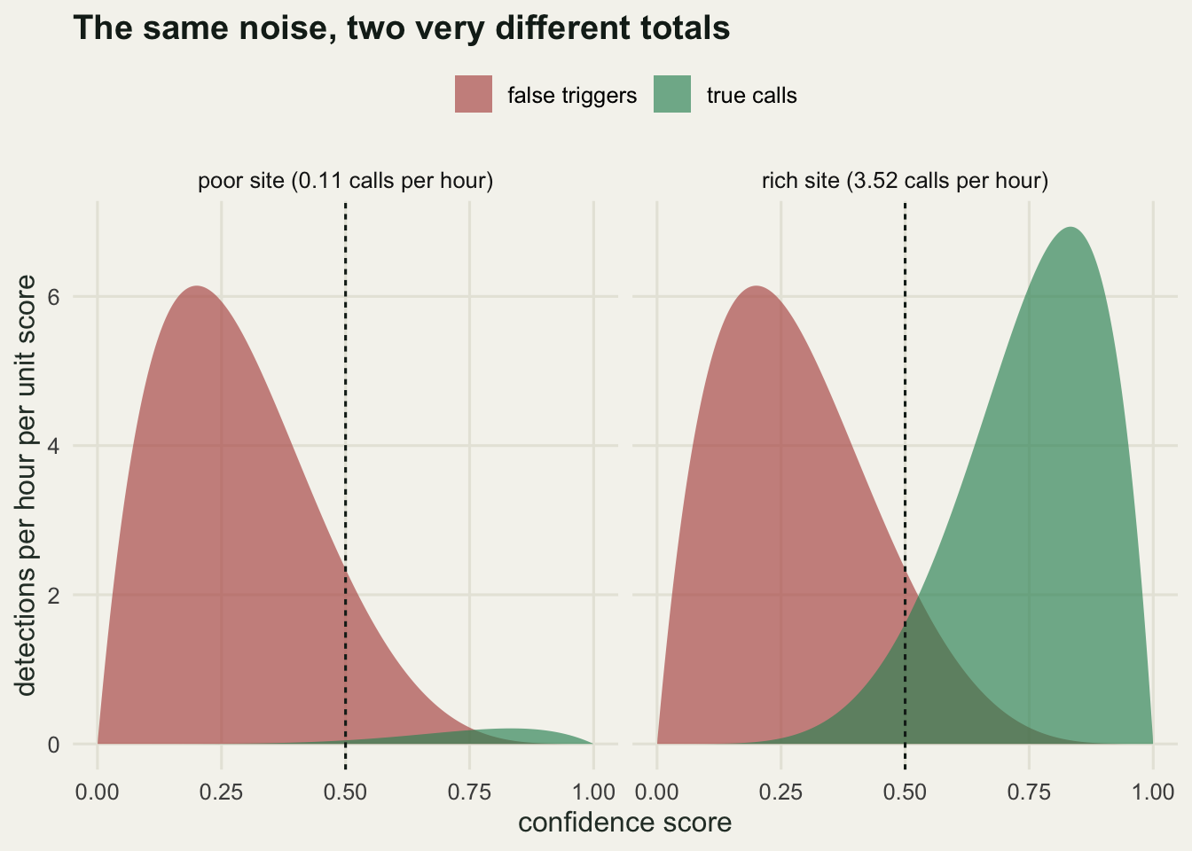

Figure 1: Composition of the detection rate by confidence score at a poor and a rich site. The noise component is identical in both panels.

The two panels share a vertical scale, so the noise curve is not merely similar between them: it is the same object, drawn from the same rate. Everything that differs between a poor site and a rich site is in the green area, and at the poor site that area is barely visible next to the noise it has to be separated from.

Detections are an affine index, not a proportional one

Regress the per-site detection count on the true call rate. The model says the expected count is hours * recall_prob * P(score > x | signal) * lambda_i plus hours * phi_false * P(score > x | noise), which is a straight line with a non-zero intercept. The intercept is the floor, in detections per site.

fit_raw <- lm(site_count ~ lambda_site)
coef_raw <- coef(fit_raw)

affine <- data.frame(
  term = c("intercept", "slope"),
  fitted = round(as.vector(coef_raw), 3),
  expected = round(c(hours_per_site * phi_false * surv_noi(thr_work),
                     hours_per_site * recall_prob * surv_sig(thr_work)), 3))
print(affine)

       term fitted expected
1 intercept  9.035    8.203
2     slope 20.022   19.688

cat("Pearson correlation of count with true rate:",
    round(cor(site_count, lambda_site), 4), "\n")

Pearson correlation of count with true rate: 0.9813 

The fit lands on both quantities, the intercept a little high in this particular survey because a single realisation of 60 Poisson counts has its own scatter. The correlation is high, which is the trap: a high correlation says the index tracks the truth monotonically, and says nothing at all about whether it tracks it proportionally. Ratios are where the difference shows up. Take two sites from the gradient and compare them the way a report would.

site_a <- 20
site_b <- 50
ratio_tab <- data.frame(
  quantity = c("true call rate ratio", "detection count ratio",
               "expected detection ratio"),
  value = round(c(
    lambda_site[site_b] / lambda_site[site_a],
    site_count[site_b] / site_count[site_a],
    det_per_hour(lambda_site[site_b], thr_work) /
      det_per_hour(lambda_site[site_a], thr_work)), 3))
print(ratio_tab)

                  quantity value
1     true call rate ratio 8.188
2    detection count ratio 5.000
3 expected detection ratio 4.026

cat("call rates compared:", round(lambda_site[site_a], 3), "and",
    round(lambda_site[site_b], 3), "calls per hour\n")

call rates compared: 0.303 and 2.481 calls per hour

cat("detection counts:", site_count[site_a], "and", site_count[site_b], "\n")

detection counts: 10 and 50 

The true call rate at site 50 is about eight times the rate at site 20. The expected detection ratio is 4.026, and this particular survey delivered exactly 5, the difference being Poisson noise on a site that produced ten detections in total. Adding a constant to both sides of a ratio pulls it towards one, and it pulls hardest when the constant is large relative to the smaller number, which is to say whenever a poor site is involved. A report that says “twice as many detections here as there” is describing something that could easily be a fourfold difference in calling.

site_df <- data.frame(lambda = lambda_site, count = site_count)
p_affine <- ggplot(site_df, aes(x = lambda, y = count)) +
  geom_abline(intercept = coef_raw[1], slope = coef_raw[2],
              colour = te_pal$clay, linewidth = 0.9) +
  geom_abline(intercept = 0, slope = coef_raw[2],
              colour = te_pal$forest, linetype = "22", linewidth = 0.7) +
  geom_hline(yintercept = coef_raw[1], colour = te_pal$gold, linetype = "12") +
  geom_point(colour = te_pal$green, size = 1.9, alpha = 0.85) +
  annotate("text", x = 3.3, y = 14, label = "false-trigger floor",
           colour = te_pal$gold, size = 3.4, hjust = 0) +
  labs(title = "The index does not start at zero",
       x = "true call rate (calls per hour)", y = "detections above threshold") +
  theme_te()
print(p_affine)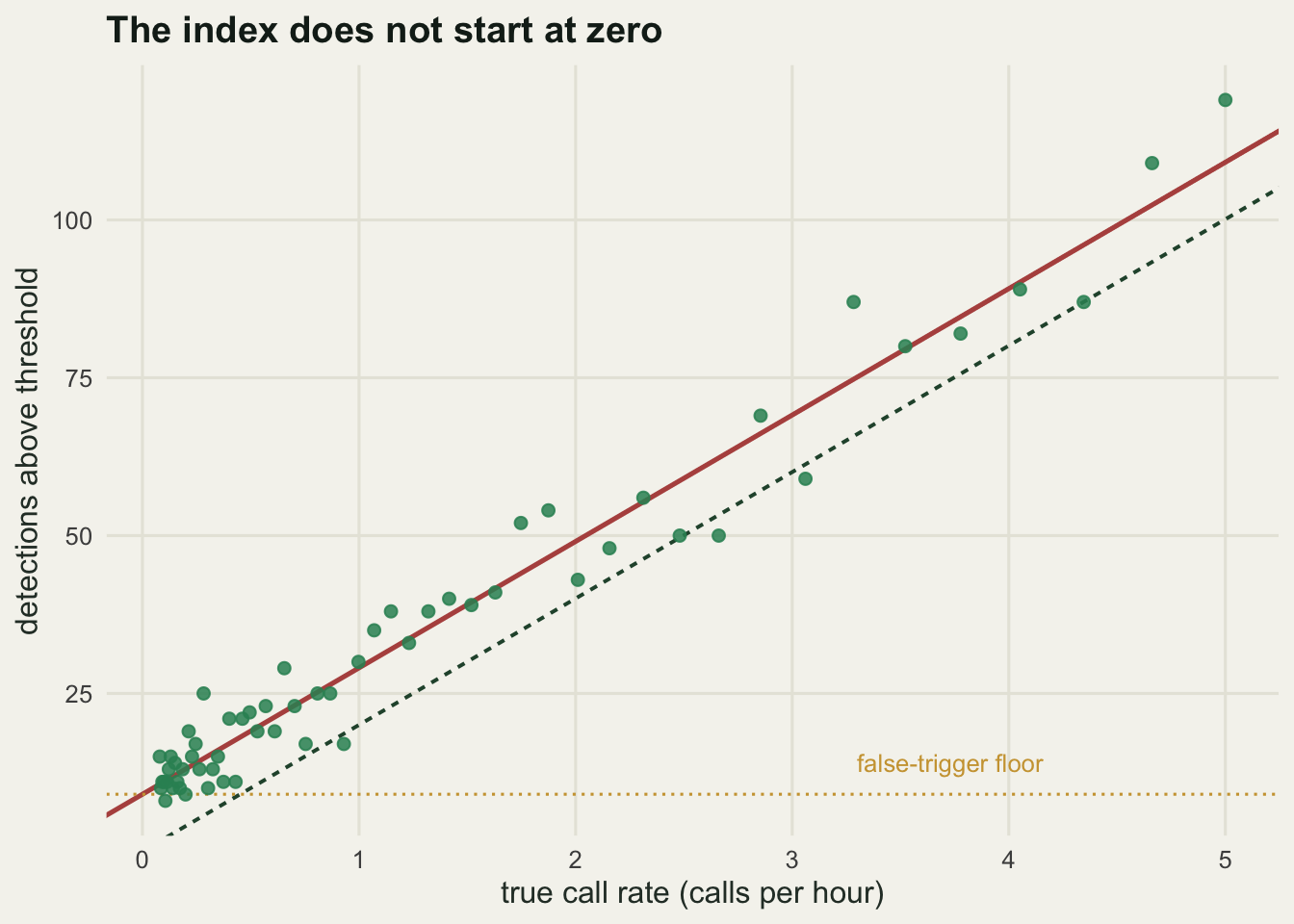

Figure 2: Detection count against true call rate across 60 sites, with the fitted affine relationship and the proportional line the fitted slope would give if there were no false triggers.

The vertical gap between the solid fitted line and the dashed line through the origin is constant in absolute terms and enormous in relative terms at the left-hand end of the gradient. That gap is what a ratio comparison silently inherits.

What raising the threshold buys and what it costs

The obvious response is to raise the score threshold until the false triggers are gone. The noise distribution has a shorter right tail than the signal distribution, so a higher threshold does remove proportionally more noise than signal. The cost is that it also throws away real detections, and a smaller count is a noisier count.

To see the trade cleanly, the survey is repeated 200 times over the same fixed gradient of sites, and each replicate is evaluated at every threshold on a grid. Repeating rather than relying on a single survey matters here: the correlation from one realisation wanders by a few hundredths, and the shape of the curve is what is being asked about.

set.seed(707)

thr_grid <- seq(0.05, 0.95, by = 0.05)
n_rep <- 200
cat("replicate surveys:", n_rep, " thresholds on the grid:", length(thr_grid), "\n")

replicate surveys: 200  thresholds on the grid: 19 

store <- array(0, c(n_rep, length(thr_grid), 6))
for (b in 1:n_rep) {
  tp <- fp <- matrix(0, n_sites, length(thr_grid))
  for (i in 1:n_sites) {
    one <- sim_scores(lambda_site[i], hours_per_site)
    s_true <- one$score[one$true_call]
    s_noise <- one$score[!one$true_call]
    tp[i, ] <- sapply(thr_grid, function(x) sum(s_true > x))
    fp[i, ] <- sapply(thr_grid, function(x) sum(s_noise > x))
  }
  for (k in seq_along(thr_grid)) {
    cnt <- tp[, k] + fp[, k]
    fit_k <- lm(cnt ~ lambda_site)
    store[b, k, 1] <- sum(tp[, k]) / max(1, sum(cnt))
    store[b, k, 2] <- sum(cnt)
    store[b, k, 3] <- coef(fit_k)[1]
    store[b, k, 4] <- coef(fit_k)[2]
    store[b, k, 5] <- cor(cnt, lambda_site)
    store[b, k, 6] <- cor(cnt, lambda_site, method = "spearman")
  }
}

sweep_tab <- data.frame(
  threshold = thr_grid,
  precision = round(apply(store[, , 1], 2, mean), 3),
  retained = round(apply(store[, , 2], 2, mean), 0),
  intercept = round(apply(store[, , 3], 2, mean), 2),
  slope = round(apply(store[, , 4], 2, mean), 2),
  pearson = round(apply(store[, , 5], 2, mean), 4),
  spearman = round(apply(store[, , 6], 2, mean), 4))
print(sweep_tab)

   threshold precision retained intercept slope pearson spearman
1       0.05     0.260     5880     72.43 21.09  0.9413   0.8601
2       0.10     0.277     5515     66.35 21.08  0.9444   0.8646
3       0.15     0.305     5023     58.14 21.09  0.9496   0.8731
4       0.20     0.342     4476     49.06 21.06  0.9546   0.8814
5       0.25     0.389     3930     39.96 21.05  0.9596   0.8909
6       0.30     0.447     3413     31.45 20.97  0.9645   0.9021
7       0.35     0.514     2949     23.87 20.84  0.9689   0.9115
8       0.40     0.589     2547     17.37 20.68  0.9725   0.9203
9       0.45     0.668     2207     12.17 20.29  0.9751   0.9292
10      0.50     0.745     1925      8.16 19.73  0.9770   0.9376
11      0.55     0.815     1683      5.15 18.88  0.9783   0.9448
12      0.60     0.875     1471      3.05 17.70  0.9783   0.9488
13      0.65     0.921     1274      1.67 16.14  0.9774   0.9502
14      0.70     0.954     1077      0.80 14.14  0.9754   0.9497
15      0.75     0.976      872      0.30 11.73  0.9716   0.9454
16      0.80     0.989      656      0.10  8.93  0.9633   0.9354
17      0.85     0.996      437      0.01  6.00  0.9483   0.9154
18      0.90     0.999      231     -0.02  3.19  0.9088   0.8715
19      0.95     1.000       68     -0.01  0.94  0.7618   0.7172

best_p <- which.max(sweep_tab$pearson)
best_s <- which.max(sweep_tab$spearman)
cat("best Pearson at threshold", sweep_tab$threshold[best_p],
    "value", sweep_tab$pearson[best_p], "\n")

best Pearson at threshold 0.55 value 0.9783 

cat("best Spearman at threshold", sweep_tab$threshold[best_s],
    "value", sweep_tab$spearman[best_s], "\n")

best Spearman at threshold 0.65 value 0.9502 

plateau <- sweep_tab$threshold[sweep_tab$pearson > sweep_tab$pearson[best_p] - 0.005]
cat("thresholds within 0.005 of the best Pearson:",
    paste(range(plateau), collapse = " to "), "\n")

thresholds within 0.005 of the best Pearson: 0.45 to 0.7 

cat("Pearson at the loosest and the tightest threshold:",
    sweep_tab$pearson[1], sweep_tab$pearson[nrow(sweep_tab)], "\n")

Pearson at the loosest and the tightest threshold: 0.9413 0.7618 

cat("precision and retained detections at the Pearson optimum:",
    sweep_tab$precision[best_p], sweep_tab$retained[best_p], "\n")

precision and retained detections at the Pearson optimum: 0.815 1683 

cat("precision and retained detections at the loosest threshold:",
    sweep_tab$precision[1], sweep_tab$retained[1], "\n")

precision and retained detections at the loosest threshold: 0.26 5880 

true_kept <- sweep_tab$precision * sweep_tab$retained
cat("share of the real detections still retained at the Pearson optimum:",
    round(true_kept[best_p] / true_kept[1], 3), "\n")

share of the real detections still retained at the Pearson optimum: 0.897 

There is an interior optimum, and it is not where precision is highest. The Pearson correlation peaks at a threshold of 0.55, where pooled precision is 0.815 and around nine tenths of the real detections are still in the table; the Spearman correlation peaks a little further along, at a threshold of 0.65. Pushing the threshold on to where precision is essentially one costs correlation, because by then the retained counts are small and Poisson noise on a small count swamps the differences between sites. The two ends of the sweep are informative in different ways: at the loosest threshold the correlation is 0.9413 with pooled precision of 0.26, and at the tightest it collapses to 0.7618 with almost nothing left to count.

The optimum is also flat. Any threshold across a wide interior band gives a correlation within half a hundredth of the best, which is worth knowing before anyone spends a week tuning a threshold to three decimal places on a validation set. What is not flat is the intercept: it falls by orders of magnitude across the same sweep, so the choice that barely moves the correlation moves the bias in a ratio comparison a great deal.

sweep_long <- rbind(
  data.frame(threshold = thr_grid, panel = "pooled precision",
             y = sweep_tab$precision),
  data.frame(threshold = thr_grid, panel = "detections retained",
             y = sweep_tab$retained),
  data.frame(threshold = thr_grid, panel = "regression intercept",
             y = sweep_tab$intercept),
  data.frame(threshold = thr_grid, panel = "Pearson correlation",
             y = sweep_tab$pearson),
  data.frame(threshold = thr_grid, panel = "Spearman correlation",
             y = sweep_tab$spearman))
panel_order <- c("pooled precision", "detections retained", "regression intercept",
                 "Pearson correlation", "Spearman correlation")
sweep_long$panel <- factor(sweep_long$panel, levels = panel_order)

p_sweep <- ggplot(sweep_long, aes(x = threshold, y = y)) +
  geom_line(colour = te_pal$forest, linewidth = 0.8) +
  geom_point(colour = te_pal$green, size = 1.2) +
  facet_wrap(~ panel, scales = "free_y", ncol = 3) +
  labs(title = "Raising the threshold trades one bias for another",
       x = "score threshold", y = NULL) +
  theme_te()
print(p_sweep)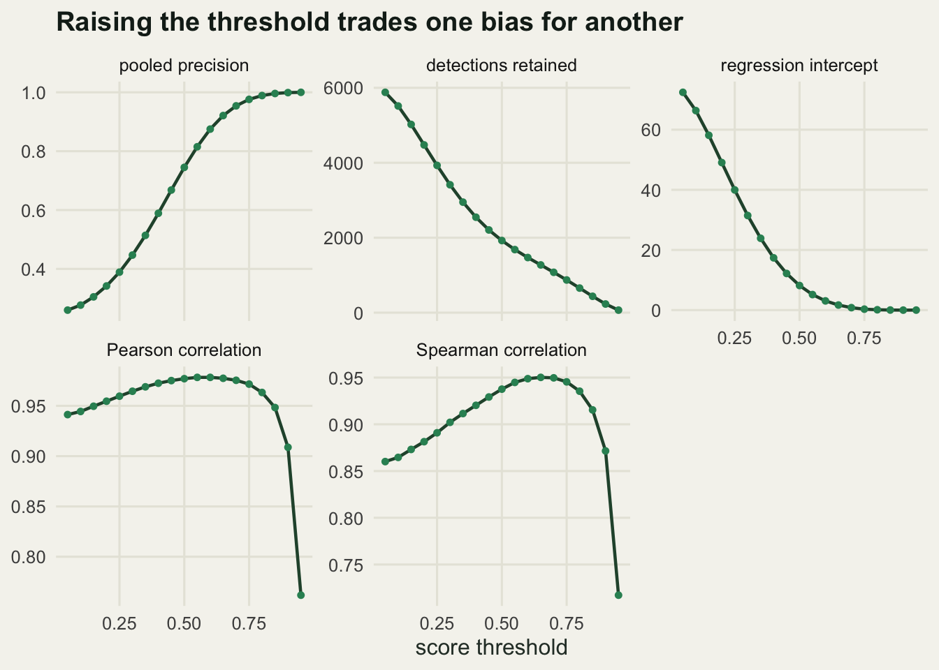

Figure 3: Five quantities across the score threshold sweep, averaged over 200 replicate surveys: pooled precision, detections retained, the regression intercept, and the two correlations of count with true call rate.

Subtracting the floor

If the floor is a constant per recorder-hour, and if it can be estimated somewhere the species is absent, it can be subtracted. That is the whole idea: run the same recogniser over recordings from sites outside the range, or from a season when the species does not call, count what comes back above the working threshold, and divide by the hours. The result estimates phi_false * P(score > x | noise) directly, which is the floor per hour.

set.seed(3021)

n_control <- 15
cat("control site-visits with no target species:", n_control, "\n")

control site-visits with no target species: 15 

control <- sim_survey(rep(0, n_control), hours_per_site)
phi_hat <- sum(control$score > thr_work) / (n_control * hours_per_site)
cat("estimated floor per hour:", round(phi_hat, 4),
    " true floor per hour:", round(phi_false * surv_noi(thr_work), 4), "\n")

estimated floor per hour: 0.2578  true floor per hour: 0.2734 

corrected <- site_count - phi_hat * hours_per_site
fit_cor <- lm(corrected ~ lambda_site)

compare <- data.frame(
  quantity = c("intercept", "slope", "Pearson correlation", "Spearman correlation"),
  raw = round(c(coef_raw[1], coef_raw[2], cor(site_count, lambda_site),
                cor(site_count, lambda_site, method = "spearman")), 6),
  corrected = round(c(coef(fit_cor)[1], coef(fit_cor)[2],
                      cor(corrected, lambda_site),
                      cor(corrected, lambda_site, method = "spearman")), 6))
print(compare)

              quantity       raw corrected
1            intercept  9.034965  1.301632
2                slope 20.021568 20.021568
3  Pearson correlation  0.981315  0.981315
4 Spearman correlation  0.931237  0.931237

The control estimate lands slightly under the true floor, and the intercept falls from about nine detections to about one while the slope does not move at all. The correlations do not move either, and the “not at all” is exact rather than approximate: subtracting the same constant from every site cannot change a correlation, ever. That is the point worth carrying away from this table: the correlation was never sensitive to the bias the correction removes, so a high correlation between an index and the truth is not evidence that the index is proportional to the truth. Two diagnostics are needed because they answer two different questions.

The residual intercept of about one detection is sampling error rather than leftover bias, in the survey and in the control estimate together. Repeating both over 100 fresh surveys shows the correction centred on zero, with a standard deviation of about one detection.

set.seed(4141)

n_rep_cor <- 100
int_raw <- int_cor <- numeric(n_rep_cor)
for (b in 1:n_rep_cor) {
  sv <- sim_survey(lambda_site, hours_per_site)
  kp <- sv[sv$score > thr_work, ]
  cnt <- as.vector(table(factor(kp$site, levels = 1:n_sites)))
  ctrl <- sim_survey(rep(0, n_control), hours_per_site)
  ph <- sum(ctrl$score > thr_work) / (n_control * hours_per_site)
  int_raw[b] <- coef(lm(cnt ~ lambda_site))[1]
  int_cor[b] <- coef(lm(cnt - ph * hours_per_site ~ lambda_site))[1]
}
cat("replicate surveys for the intercept check:", n_rep_cor, "\n")

replicate surveys for the intercept check: 100 

cat("mean raw intercept:", round(mean(int_raw), 3),
    " mean corrected intercept:", round(mean(int_cor), 3), "\n")

mean raw intercept: 8.194  mean corrected intercept: -0.111 

cat("sd of the corrected intercept:", round(sd(int_cor), 3), "\n")

sd of the corrected intercept: 1.06 

The ratio is the quantity that does move. Because a single survey gives a single noisy ratio, the recovery is measured over 200 replicate surveys, each with its own independent control estimate of the floor.

set.seed(88)

n_ratio <- 200
raw_ratio <- corr_ratio <- numeric(n_ratio)
for (b in 1:n_ratio) {
  ca <- sum(sim_scores(lambda_site[site_a], hours_per_site)$score > thr_work)
  cb <- sum(sim_scores(lambda_site[site_b], hours_per_site)$score > thr_work)
  ctrl <- sim_survey(rep(0, n_control), hours_per_site)
  ph <- sum(ctrl$score > thr_work) / (n_control * hours_per_site)
  raw_ratio[b] <- cb / ca
  corr_ratio[b] <- (cb - ph * hours_per_site) / (ca - ph * hours_per_site)
}

true_ratio <- lambda_site[site_b] / lambda_site[site_a]
recovery <- data.frame(
  quantity = c("true call rate ratio", "median raw ratio", "median corrected ratio",
               "10th percentile corrected", "90th percentile corrected"),
  value = round(c(true_ratio, median(raw_ratio), median(corr_ratio),
                  quantile(corr_ratio, 0.1), quantile(corr_ratio, 0.9)), 3))
print(recovery)

                   quantity  value
1      true call rate ratio  8.188
2          median raw ratio  4.138
3    median corrected ratio  7.762
4 10th percentile corrected  3.420
5 90th percentile corrected 25.137

cat("replicates where the corrected ratio is negative or undefined:",
    sum(!is.finite(corr_ratio) | corr_ratio < 0), "\n")

replicates where the corrected ratio is negative or undefined: 15 

The correction works in the middle and is expensive in the tails. The median corrected ratio lands close to the truth while the median raw ratio is compressed by roughly a factor of two, but the spread of the corrected ratio is wide: the middle 80 percent of replicates runs from 3.42 up to 25.14, and 15 of the 200 replicates gave a value that was negative or undefined. The reason is the denominator, a small count minus an estimated constant of similar size, which is sometimes near zero and occasionally the wrong side of it. Correcting a low-density site turns a confident wrong answer into an honest uncertain one, which is progress, but nobody should report the corrected ratio without its interval.

idx_df <- rbind(
  data.frame(lambda = lambda_site, y = site_count, kind = "raw detection count"),
  data.frame(lambda = lambda_site, y = corrected, kind = "floor subtracted"))
kind_order <- c("raw detection count", "floor subtracted")
idx_df$kind <- factor(idx_df$kind, levels = kind_order)
fit_lines <- data.frame(kind = factor(kind_order, levels = kind_order),
                        b0 = c(coef_raw[1], coef(fit_cor)[1]),
                        b1 = c(coef_raw[2], coef(fit_cor)[2]))

p_cor <- ggplot(idx_df, aes(x = lambda, y = y)) +
  geom_hline(yintercept = 0, colour = te_pal$sage) +
  geom_abline(intercept = 0, slope = coef_raw[2],
              colour = te_pal$forest, linetype = "22", linewidth = 0.7) +
  geom_abline(data = fit_lines, aes(intercept = b0, slope = b1),
              colour = te_pal$clay, linewidth = 0.9) +
  geom_point(colour = te_pal$green, size = 1.8, alpha = 0.85) +
  facet_wrap(~ kind) +
  labs(title = "Subtracting an estimated floor restores proportionality",
       x = "true call rate (calls per hour)", y = "index value") +
  theme_te()
print(p_cor)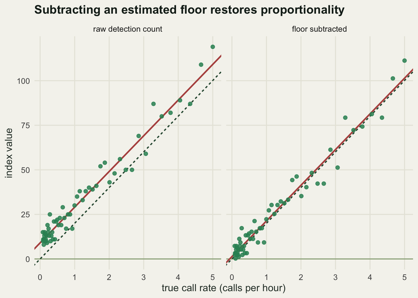

Figure 4: Raw and floor-subtracted detection counts against true call rate, each with its own fitted line and a dashed reference line of the same slope through the origin. Only the corrected index sits on the reference line.

What this cannot tell you

The detection table does not identify recall. The relationship between expected count and true call rate has two unknowns, a slope and an intercept, and the slope is the recorder hours times recall times the probability that a real call scores above the threshold. Hours are known and the other two are not, so the survey sees only that product. Doubling recall and halving the true call rates everywhere gives detection counts with the same expectation, so no amount of staring at the detection table separates them. Recall has to come from somewhere else: annotated clips with known calls, a validation set from a comparable habitat, or a paired human count on the same recordings.

That is less damaging than it sounds for relative work and completely damaging for absolute work. A recall that is constant across sites cancels out of every ratio, so the compression described above is caused by the floor and not by recall. If the aim is a statement about absolute calling rate or absolute density, the same constant multiplies everything and the answer is wrong by exactly that factor, with nothing in the data to reveal it.

There is a second assumption doing quiet work throughout. The false-trigger rate has been treated as one number per hour, constant across sites and across time. Real false triggers are driven by weather, by season, by the acoustic character of the site and by which congeners are around, so the floor varies in ways that correlate with the very habitat gradients an ecologist wants to study. A floor that is higher in windy open sites and lower in sheltered forest sites does not subtract cleanly, and it can manufacture an apparent habitat effect out of nothing. The fourth tutorial in this cluster takes that assumption apart deliberately.

A third limit is smaller but easy to trip over: the model assumes each call is scored independently. Real recognisers process overlapping windows, a single long song can produce several rows, and calls cluster in bouts, so the effective count has more variance than a Poisson process would give. That inflates the noise on every correlation reported here without changing the direction of any of the results.

Where to go next

The threshold sweep here treated precision as one number in a table. It deserves more than that, because the choice of threshold is the single decision that most changes what an acoustic dataset says, and because precision measured on a validation set is not the precision the survey actually gets. The next tutorial in this cluster, score thresholds and precision in bioacoustics, builds the score distributions from the recogniser side, derives precision and recall as functions of the threshold and of how common the species is, and shows why the same threshold gives different precision at a common site and a rare one.

References

Shonfield J, Bayne EM 2017 Avian Conservation and Ecology 12(1):14 (10.5751/ACE-00974-120114)

Sugai LSM, Silva TSF, Ribeiro JW, Llusia D 2019 BioScience 69(1):15-25 (10.1093/biosci/biy147)

Knight EC, Hannah KC, Foley GJ, Scott CD, Brigham RM, Bayne EM 2017 Avian Conservation and Ecology 12(2):14 (10.5751/ACE-01114-120214)

Royle JA, Link WA 2006 Ecology 87(4):835-841 (10.1890/0012-9658(2006)87[835:GSOMAF]2.0.CO;2)

Priyadarshani N, Marsland S, Castro I 2018 Journal of Avian Biology 49(5):jav-01447 (10.1111/jav.01447)

Related tutorials

• Score thresholds and precision in bioacoustics
• Call rates and density from acoustic surveys
• Checking an acoustic monitoring analysis
• False positives in occupancy models