library(ggplot2)

te_paper  <- "#f5f4ee"
te_ink    <- "#16241d"
te_body   <- "#2c3a31"
te_forest <- "#275139"
te_rust   <- "#b5534e"
te_gold   <- "#c9b458"
te_line   <- "#dad9ca"

theme_datasheet <- function() {
  theme_minimal(base_size = 12) +
    theme(plot.background  = element_rect(fill = te_paper, colour = NA),
          panel.background = element_rect(fill = te_paper, colour = NA),
          panel.grid.major = element_line(colour = te_line, linewidth = 0.3),
          panel.grid.minor = element_blank(),
          text             = element_text(colour = te_body),
          plot.title       = element_text(colour = te_ink, face = "bold"),
          plot.subtitle    = element_text(colour = te_body),
          axis.text        = element_text(colour = te_body))
}Acoustic indices and species richness
R
bioacoustics
acoustic monitoring
biodiversity
simulation
ecology tutorial
Acoustic entropy and the ACI on simulated spectrograms in R: the sign of their link to species richness follows the noise floor, call energy and note length.
A set of autonomous recorders sits along a gradient from an old forest interior to a logged edge beside a gravel road. Nobody has time to identify every call in three months of audio, so each recording is reduced to a handful of numbers: the acoustic entropy index H of Sueur and colleagues, the acoustic complexity index ACI of Pieretti and colleagues, sometimes a few more. The numbers go into a regression against the bird point counts, and the hope is that a positive slope turns the recorders into a richness survey.
The acoustic posts on this site so far keep species identity. Automated acoustic detections as data simulates a recogniser and shows that detection counts are an affine index of true call rate, with a false-trigger floor underneath. Call rates and density from acoustic surveys turns those species-level cues into a density. Checking an acoustic monitoring analysis shows that a score threshold tuned at a quiet site does not travel to a noisy one, and mentions a spectrogram only as something to look at when auditing. A soundscape index drops species identity altogether: it summarises how sound energy is spread across time and frequency. This post measures what that summary is reading, by building spectrograms whose communities are known exactly and changing one thing at a time.
A spectrogram built from known communities
No audio is synthesised here. The recording is represented directly as its short-time Fourier transform magnitude: a matrix with 63 frequency bins and 240 time frames. The regional pool has 21 species, and each species owns a band of 3 adjacent bins, so bands never overlap and two species can never mask each other. A call is a small template of power added to the species band at a random start frame. Each species at a site gets a call amplitude drawn once from a lognormal distribution, because some birds are close to the microphone and some are not.
Background noise is added in power. Where there is no call, the noise power in a cell is exponential, which is what the squared magnitude of Gaussian noise in a Fourier bin is; the magnitude itself is then Rayleigh. Adding signal power and noise power and taking the square root ignores the phase between them, which is the main simplification: a real cell with both is Rician. The noise level is set as a signal to noise ratio, in decibels, relative to the median call peak power of one.
n_freq   <- 63      # frequency bins
n_frame  <- 240     # time frames
n_pool   <- 21      # species in the regional pool
band_w   <- 3       # bins per species band
step_len <- 24      # frames per ACI temporal step (ten steps)
amp_sd   <- 0.5     # sd of log call amplitude among species
calls_each  <- 4    # chorus design: calls per species per recording
calls_total <- 40   # fixed-energy design: calls per recording, shared out
snr_db   <- c(40, 35, 30, 25, 20, 15, 10)
n_survey <- 10      # replicate surveys per scenario
n_sites  <- 40      # sites per survey, richness uniform on 1 to 21

call_template <- function(kind) {
  switch(kind,
    smooth = outer(c(0.5, 1, 0.5), sin(pi * (1:6 - 0.5) / 6))^2,
    pulsed = outer(c(0.5, 1, 0.5), rep(c(1, 0.15), 3))^2,
    tonal  = rbind(0, sin(pi * (1:12 - 0.5) / 12), 0)^2,
    short  = outer(c(0.5, 1, 0.5), sin(pi * (1:2 - 0.5) / 2))^2,
    sweep  = cbind(diag(3), diag(3)[3:1, ]))
}
noise_profile <- function(kind) {
  if (kind == "white") return(rep(1, n_freq))
  w_low <- 1 / seq_len(n_freq)^0.8          # wind: power falls with frequency
  w_low / mean(w_low)
}
The smooth call is a six frame note with a sine envelope, the default for everything below. The pulsed call is the same length but switches between full and low amplitude every frame, like a trill. The tonal call is a twelve frame whistle confined to the middle bin of its band. These three and the two noise profiles were fixed before any index was computed; the point of having them is to see which conclusions survive a change of template or noise. Two more templates were added after a first round of results, to test a claim about the ACI: a short note, the smooth note cut to two frames, and a sweep that climbs across the three bins of its band one frame per bin and comes back down, which holds the top bin for two frames.
make_signal <- function(rich, rate_fun, tmpl) {
  n_s <- length(rich); tf <- nrow(tmpl); tt <- ncol(tmpl)
  site_of <- rep(seq_len(n_s), rich)
  sp_of   <- unlist(lapply(rich, function(s) sample.int(n_pool, s)))
  k_calls <- rpois(length(sp_of), rate_fun(rich)[site_of])
  amp2    <- exp(rnorm(length(sp_of), 0, amp_sd))^2
  c_site <- rep(site_of, k_calls); c_sp <- rep(sp_of, k_calls)
  c_amp2 <- rep(amp2, k_calls); n_call <- length(c_site)
  c_start <- sample.int(n_frame - tt + 1, n_call, replace = TRUE)
  cells  <- tf * tt
  f_idx <- rep((c_sp - 1) * band_w, each = cells) + rep(seq_len(tf) - 1, times = tt) + 1
  t_idx <- rep(c_start, each = cells) + rep(seq_len(tt) - 1, each = tf)
  s_idx <- rep(c_site, each = cells)
  lin   <- s_idx + (f_idx - 1) * n_s + (t_idx - 1) * n_s * n_freq
  pow   <- numeric(n_s * n_freq * n_frame)
  if (n_call > 0) {
    summed <- rowsum(rep(c_amp2, each = cells) * as.vector(tmpl), lin)
    pow[as.integer(rownames(summed))] <- summed[, 1]
  }
  array(pow, c(n_s, n_freq, n_frame))   # site x frequency x frame, power
}
chorus_rate <- function(rich) rep(calls_each, length(rich))
fixed_rate  <- function(rich) calls_total / rich
In the chorus design every species present calls at the same expected rate, so a richer site is also a louder, busier site. In the fixed-energy design the same expected number of calls is shared among however many species are present, so richness changes how the energy is distributed but not how much of it there is.
The two indices, as their authors define them
Sueur and colleagues 2008 define the temporal entropy Ht from the amplitude envelope of the waveform, normalised to sum to one over time, and the spectral entropy Hf from the mean amplitude spectrum of a short-time Fourier transform, normalised to sum to one over frequency. Each is a Shannon entropy divided by its maximum, the log of the number of elements, and H is the product of the two. The envelope in the paper comes from the Hilbert transform at sample resolution. A spectrogram has no samples, so the envelope here is the root mean square amplitude of each frame, the square root of the summed squared magnitudes across bins, which by Parseval’s theorem is proportional to the waveform root mean square in that frame. That is a coarser envelope than the Hilbert one, and it is the one approximation in H.
Pieretti and colleagues 2011 define the ACI on the same magnitude matrix. In each frequency bin, within each temporal step, the absolute differences between successive intensities are summed and divided by the sum of the intensities in that step; the result is summed over steps to give the value for the bin, and over bins to give the total.
row_entropy <- function(mat) {
  p_mat <- mat / rowSums(mat)
  -rowSums(ifelse(p_mat > 0, p_mat * log(p_mat), 0)) / log(ncol(mat))
}
soundscape_indices <- function(amp) {                 # amp: site x frequency x frame
  envelope <- sqrt(rowSums(aperm(amp^2, c(1, 3, 2)), dims = 2))
  h_t <- row_entropy(envelope)
  h_f <- row_entropy(rowSums(amp, dims = 2) / n_frame)
  aci <- numeric(dim(amp)[1])
  for (j in seq_len(n_frame %/% step_len)) {
    frames <- (j - 1) * step_len + seq_len(step_len)
    blk <- amp[, , frames, drop = FALSE]
    d_sum <- rowSums(abs(blk[, , -1, drop = FALSE] - blk[, , -step_len, drop = FALSE]), dims = 2)
    aci <- aci + rowSums(d_sum / rowSums(blk, dims = 2))
  }
  data.frame(H = h_t * h_f, Ht = h_t, Hf = h_f, ACI = aci)
}
Noise is drawn once per site and scaled to each level, so the sites at 40 dB and at 10 dB carry the same calls and the same noise pattern, only louder. Every difference between levels is the level.
set.seed(311)
demo_rich <- c(3, 18)
demo_pow  <- make_signal(demo_rich, chorus_rate, call_template("smooth"))
demo_noise <- array(rexp(length(demo_pow)), dim(demo_pow))
demo_df <- do.call(rbind, lapply(c(40, 15), function(db) {
  amp <- sqrt(demo_pow + 10^(-db / 10) * demo_noise)
  do.call(rbind, lapply(1:2, function(i) {
    data.frame(frame = rep(seq_len(n_frame), each = n_freq),
               bin = rep(seq_len(n_freq), n_frame),
               level_db = 20 * log10(as.vector(amp[i, , ])),
               panel = sprintf("%d species, %d dB", demo_rich[i], db))
  }))
}))
demo_df$panel <- factor(demo_df$panel, levels = unique(demo_df$panel))
ggplot(demo_df, aes(frame, bin, fill = pmax(level_db, -30))) +
  geom_raster() +
  facet_wrap(~ panel, ncol = 2) +
  scale_fill_gradient(low = te_paper, high = te_ink, name = "magnitude\n(dB)") +
  labs(x = "time frame", y = "frequency bin") +
  theme_datasheet() +
  theme(strip.text = element_text(colour = te_ink, face = "bold"))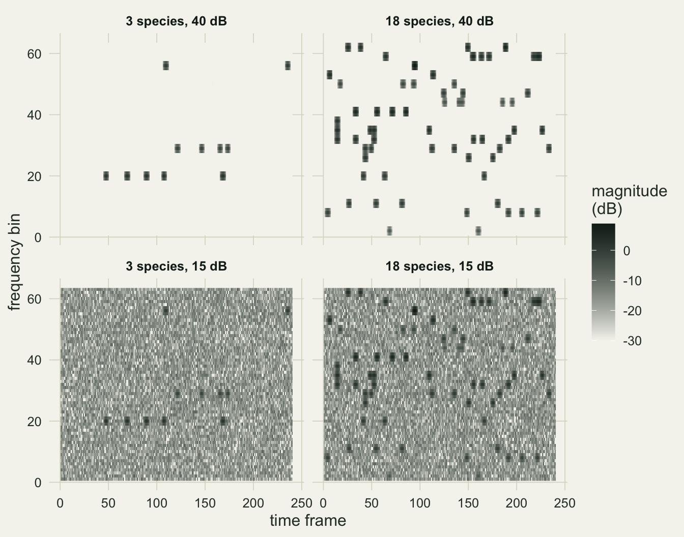
The same communities, seven noise floors
The first experiment is the chorus design with smooth calls and white noise. Each of 10 replicate surveys draws 40 sites with richness uniform between 1 and 21, and the Spearman rank correlation between each index and richness is computed within the survey. The mean over surveys is the estimate and the spread among surveys gives its Monte Carlo standard error.
run_scenario <- function(rate_fun, tkind, nkind, levels_db, seed) {
  set.seed(seed)
  tmpl <- call_template(tkind); prof <- noise_profile(nkind)
  out <- vector("list", n_survey)
  for (s in seq_len(n_survey)) {
    rich <- sample.int(n_pool, n_sites, replace = TRUE)
    pow <- make_signal(rich, rate_fun, tmpl)
    noise <- array(rexp(length(pow)), dim(pow)) * rep(prof, each = n_sites)
    energy <- rowSums(pow)
    out[[s]] <- do.call(rbind, lapply(levels_db, function(db) {
      ix <- soundscape_indices(sqrt(pow + 10^(-db / 10) * noise))
      data.frame(survey = s, snr = db, index = names(ix),
                 rho = vapply(ix, function(v) cor(v, rich, method = "spearman"), 0),
                 rho_energy = cor(energy, rich, method = "spearman"))
    }))
  }
  do.call(rbind, out)
}
summarise_rho <- function(res) {
  agg <- aggregate(rho ~ snr + index, data = res, FUN = mean)
  agg$mcse <- aggregate(rho ~ snr + index, data = res,
                        FUN = function(v) sd(v) / sqrt(length(v)))$rho
  agg$share_neg <- aggregate(rho ~ snr + index, data = res,
                             FUN = function(v) mean(v < 0))$rho
  agg
}
pick <- function(agg, idx, db, col = "rho") agg[agg$index == idx & agg$snr == db, col]
t_start <- proc.time()[["elapsed"]]
res_chorus <- run_scenario(chorus_rate, "smooth", "white", snr_db, seed = 3111)
agg_chorus <- summarise_rho(res_chorus)
rho_energy_chorus <- mean(res_chorus$rho_energy)
h_quiet <- pick(agg_chorus, "H", 40); h_noisy <- pick(agg_chorus, "H", 10)
h_quiet_se <- pick(agg_chorus, "H", 40, "mcse"); h_noisy_se <- pick(agg_chorus, "H", 10, "mcse")
ht_quiet <- pick(agg_chorus, "Ht", 40); ht_noisy <- pick(agg_chorus, "Ht", 10)
hf_quiet <- pick(agg_chorus, "Hf", 40); hf_noisy <- pick(agg_chorus, "Hf", 10)
h_rows <- agg_chorus[agg_chorus$index == "H", ]
h_cross <- max(h_rows$snr[h_rows$rho < 0]) # quietest level with a negative mean
share_neg_quiet <- pick(agg_chorus, "H", 40, "share_neg")
share_neg_noisy <- pick(agg_chorus, "H", 10, "share_neg")
max_mcse <- max(agg_chorus$mcse[agg_chorus$index != "ACI"])Richness and total call energy are rank correlated at 0.81 in this design, which is the point of it: in a real chorus more species means more sound. At 40 dB the mean rank correlation between H and richness is 0.67 (Monte Carlo standard error 0.03), and 0 per cent of surveys give a negative value. At 10 dB, with exactly the same calls, it is -0.62 (standard error 0.02), and 100 per cent of surveys are negative. The mean is already negative at 25 dB. The largest standard error for the entropy indices in this scenario is 0.054.
set.seed(3113)
size_rich  <- rep(seq_len(n_pool), each = 15)      # 15 sites at each richness value
size_pow   <- make_signal(size_rich, chorus_rate, call_template("smooth"))
size_noise <- array(rexp(length(size_pow)), dim(size_pow))
size_by_rich <- lapply(c(q = 40, n = 10), function(db) {
  ix <- soundscape_indices(sqrt(size_pow + 10^(-db / 10) * size_noise))
  sapply(ix, function(v) tapply(v, size_rich, mean))  # richness x index means
})
h_span       <- sapply(size_by_rich, function(m) diff(range(m[, "H"])))
h_level_mean <- sapply(size_by_rich, function(m) mean(m[, "H"]))
h_noisy_ends <- size_by_rich$n[c(1, n_pool), "H"]
ht_q_by_rich <- size_by_rich$q[, "Ht"]
ht_q_min_at  <- which.min(ht_q_by_rich)
A rank correlation says nothing about size. With 15 sites at each richness value from 1 to 21, the mean H of the richness classes spans 0.165 at 40 dB and 0.004 at 10 dB, where it goes from 0.999 with one species to 0.997 with 21. The negative correlation at the noisy level is real as a rank order, but it sits in the third decimal of an index pressed against its maximum of one. The level itself moves the average H over all classes from 0.828 to 0.997.
ent_rows <- agg_chorus[agg_chorus$index != "ACI", ]
ent_rows$index <- factor(ent_rows$index, levels = c("H", "Ht", "Hf"))
ggplot(ent_rows, aes(snr, rho, colour = index)) +
  geom_hline(yintercept = 0, colour = te_body, linetype = "dashed") +
  geom_line(linewidth = 0.9) + geom_point(size = 2) +
  geom_errorbar(aes(ymin = rho - 2 * mcse, ymax = rho + 2 * mcse), width = 0.8) +
  scale_x_reverse(breaks = snr_db) +
  scale_colour_manual(values = c(H = te_ink, Ht = te_rust, Hf = te_gold), name = NULL) +
  coord_cartesian(ylim = c(-1, 1)) +
  labs(x = "signal to noise ratio (dB), quieter to noisier", y = "Spearman correlation with richness") +
  theme_datasheet() + theme(legend.position = "top")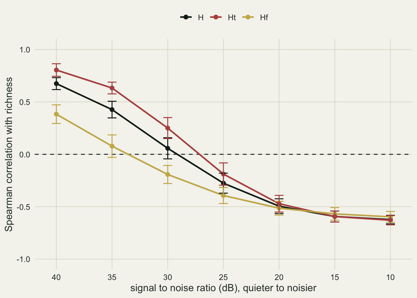
The two components say why. In a quiet recording the floor envelope is low, so beyond a few species each added species fills in more of the time axis and Ht rises with richness (0.80). The low end is not monotone: in the 15 sites per class above, mean Ht at 40 dB is 0.877 with one species, falls to 0.861 at 3 species and reaches 0.957 with 21, because the first few species add isolated peaks to a nearly flat floor envelope before the calls start to fill it. Once the noise floor gives every frame a similar envelope, calls become peaks sticking out of a flat line, and more calls make the envelope less even (-0.63). The spectral side does the same thing along the frequency axis: Hf goes from 0.38 at 40 dB to -0.60 at 10 dB, because a flat noise spectrum is already maximally even and every occupied band makes it lumpier. In this design H is reading how far the calls stand out from the background, and here that grows with richness.
Take the energy out of richness
The chorus design ties richness to call energy. The fixed-energy design shares out the same expected number of calls, so the question is whether the flip needs that tie.
res_fixed <- run_scenario(fixed_rate, "smooth", "white", snr_db, seed = 3112)
agg_fixed <- summarise_rho(res_fixed)
rho_energy_fixed <- mean(res_fixed$rho_energy)
hfx_quiet <- pick(agg_fixed, "H", 40); hfx_noisy <- pick(agg_fixed, "H", 10)
htfx_quiet <- pick(agg_fixed, "Ht", 40); hffx_quiet <- pick(agg_fixed, "Hf", 40)
hffx_noisy <- pick(agg_fixed, "Hf", 10)
hfx_min <- min(agg_fixed$rho[agg_fixed$index == "H"])
hfx_min_se <- agg_fixed$mcse[agg_fixed$index == "H"][which.min(agg_fixed$rho[agg_fixed$index == "H"])]
Here total call energy and richness are rank correlated at only 0.21. That residue comes from the skewed amplitudes: with one or two species the total is dominated by one or two lognormal draws, so its median is lower even though its expectation is not. H and richness correlate at 0.82 at 40 dB and 0.22 at 10 dB, and the lowest mean at any level is 0.19 (standard error 0.04). There is no flip. The spectral entropy carries the richness signal (0.89 at 40 dB, 0.58 at 10 dB), because the same energy spread over more bands is a more even spectrum, and the temporal entropy is weakly negative throughout (-0.24 at 40 dB).
both <- rbind(data.frame(h_rows, design = "chorus: energy grows with richness"),
              data.frame(agg_fixed[agg_fixed$index == "H", ], design = "fixed energy: shared among species"))
ggplot(both, aes(snr, rho, colour = design)) +
  geom_hline(yintercept = 0, colour = te_body, linetype = "dashed") +
  geom_line(linewidth = 0.9) + geom_point(size = 2) +
  geom_errorbar(aes(ymin = rho - 2 * mcse, ymax = rho + 2 * mcse), width = 0.8) +
  scale_x_reverse(breaks = snr_db) +
  scale_colour_manual(values = c(te_rust, te_forest), name = NULL) +
  coord_cartesian(ylim = c(-1, 1)) +
  labs(x = "signal to noise ratio (dB), quieter to noisier", y = "Spearman correlation of H with richness") +
  theme_datasheet() + theme(legend.position = "top", legend.direction = "vertical")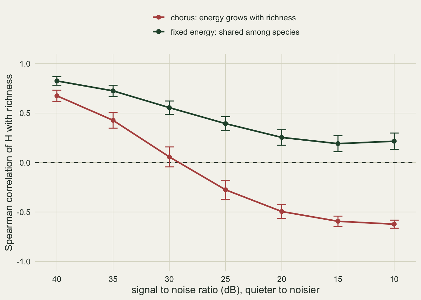
So the sign flip in the first experiment is not H responding to richness in two opposite ways. It is H responding to call energy relative to the noise floor, which in a chorus happens to rise with richness. Field data are chorus data: a site with more species usually has more calling, and a site near a road usually has a higher floor. Both designs are the same communities in the sense that matters for a richness survey; only the second lets the index show what it does with richness alone.
Other calls, other noise
A result that holds for one call shape and one noise spectrum could be a feature of that shape. The chorus design is rerun with the pulsed and tonal calls, and with a low-frequency noise profile standing in for wind, at four levels.
variant_grid <- expand.grid(tkind = c("smooth", "pulsed", "tonal"), nkind = c("white", "wind"),
                            stringsAsFactors = FALSE)
variant_db <- c(40, 30, 20, 10)
res_var <- do.call(rbind, lapply(seq_len(nrow(variant_grid)), function(i) {
  agg <- summarise_rho(run_scenario(chorus_rate, variant_grid$tkind[i], variant_grid$nkind[i],
                                    variant_db, seed = 3120 + i))
  cbind(agg, call = variant_grid$tkind[i], noise = variant_grid$nkind[i])
}))
pick_var <- function(idx, tk, nk, db, col = "rho")
  res_var[res_var$index == idx & res_var$call == tk & res_var$noise == nk & res_var$snr == db, col]
h_white <- sapply(c("smooth", "pulsed", "tonal"), function(tk) c(q = pick_var("H", tk, "white", 40),
                                                                  n = pick_var("H", tk, "white", 10)))
h_wind <- sapply(c("smooth", "pulsed", "tonal"), function(tk) sapply(variant_db, function(db) pick_var("H", tk, "wind", db)))
hf_wind_noisy <- pick_var("Hf", "smooth", "wind", 10); ht_wind_noisy <- pick_var("Ht", "smooth", "wind", 10)
hf_tonal_quiet <- pick_var("Hf", "tonal", "white", 40); ht_tonal_quiet <- pick_var("Ht", "tonal", "white", 40)
hf_tonal_wind_noisy <- pick_var("Hf", "tonal", "wind", 10)
var_mcse <- max(res_var$mcse[res_var$index == "H"])
seed_diff <- c(pick_var("H", "smooth", "white", 40) - h_quiet, pick_var("H", "smooth", "white", 10) - h_noisy)
seed_z <- abs(seed_diff) / sqrt(c(pick_var("H", "smooth", "white", 40, "mcse")^2 + h_quiet_se^2,
                                  pick_var("H", "smooth", "white", 10, "mcse")^2 + h_noisy_se^2))
h_var <- res_var[res_var$index == "H", ]
h_var$call <- factor(h_var$call, levels = c("smooth", "pulsed", "tonal"))
ggplot(h_var, aes(snr, rho, colour = noise)) +
geom_hline(yintercept = 0, colour = te_body, linetype = "dashed") +
geom_line(linewidth = 0.9) + geom_point(size = 2) +
geom_errorbar(aes(ymin = rho - 2 * mcse, ymax = rho + 2 * mcse), width = 1.2) +
facet_wrap(~ call, ncol = 3) +
scale_x_reverse(breaks = variant_db) +
scale_colour_manual(values = c(white = te_ink, wind = te_gold), name = "noise") +
coord_cartesian(ylim = c(-1, 1)) +
labs(x = "signal to noise ratio (dB)", y = "Spearman correlation of H with richness") +
theme_datasheet() +
theme(legend.position = "top", strip.text = element_text(colour = te_ink, face = "bold"))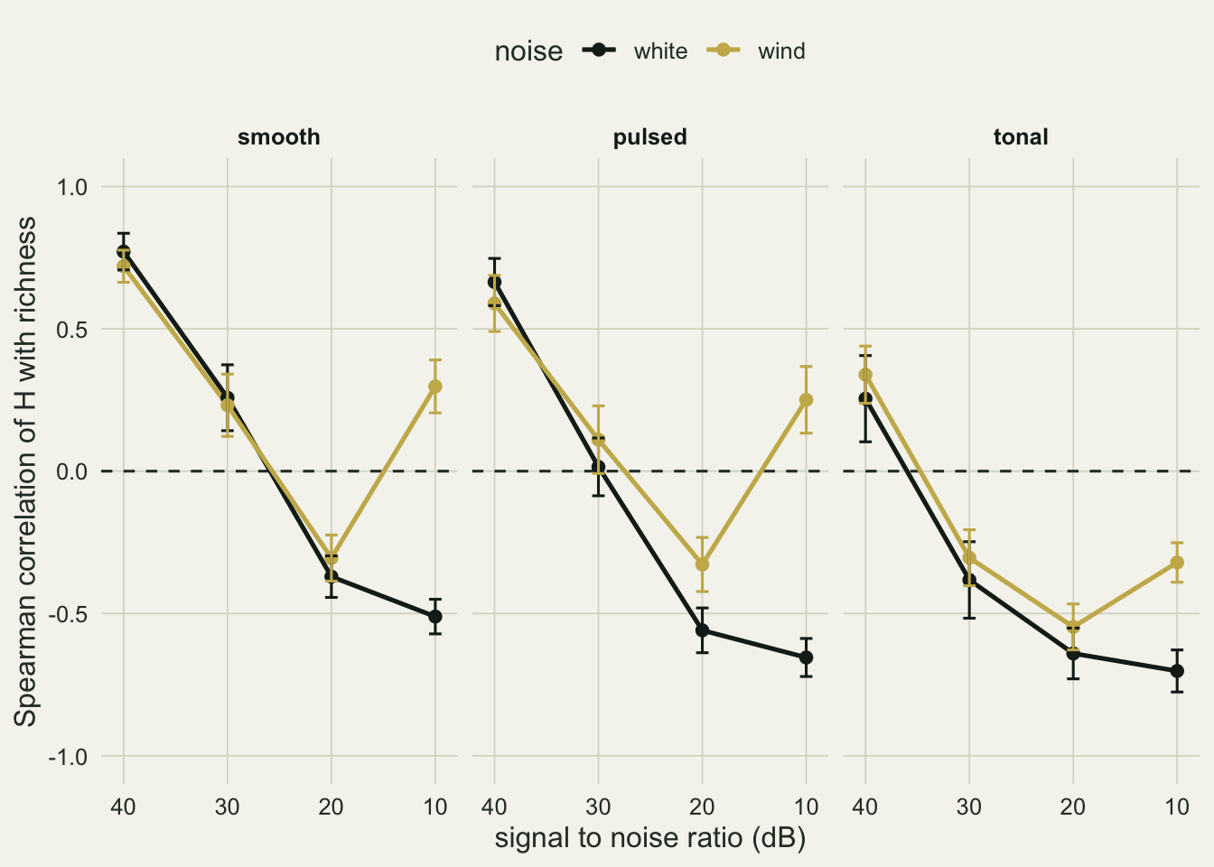
Under white noise the flip survives both changes of call: from 40 dB to 10 dB the correlation goes from 0.77 to -0.51 for smooth calls, 0.66 to -0.65 for pulsed calls and 0.25 to -0.70 for tonal whistles. The quiet positive value is weakest for the whistles, and it comes from the time axis alone: at 40 dB their Ht correlates with richness at 0.84 and their Hf at -0.13, because a one bin whistle adds a narrow spike to the mean spectrum rather than filling a band. The largest standard error for H in this set is 0.08. The smooth, white-noise row repeats the first experiment with new draws, and it differs from it by 0.10 at 40 dB and 0.11 at 10 dB, which is 2.2 and 3.1 times the combined standard error of the two estimates.
Wind noise does not behave like white noise. With smooth calls the correlation runs 0.72, 0.23, -0.31, 0.30 across 40, 30, 20 and 10 dB. Low-frequency noise makes the spectrum uneven before any bird calls, and calls spread across the bands fill in the quiet upper part of the spectrum, where the wind is weak; at 10 dB Hf correlates with richness at 0.59 while Ht stays at -0.65. Pulsed calls follow the same pattern (0.59, 0.11, -0.33, 0.25). Tonal whistles do not recover at 10 dB (0.34, -0.30, -0.55, -0.32): a one bin spike does not even out the spectrum, and their Hf correlation at 10 dB is -0.19. The direction of the H to richness relation is then set by the noise spectrum and the call shape as well as the noise level, and a monotone story about a rising floor does not hold.
ACI reads how long a note holds a bin
aci_white <- sapply(c("smooth", "pulsed", "tonal"), function(tk) sapply(variant_db, function(db) pick_var("ACI", tk, "white", db)))
aci_fixed_quiet <- pick(agg_fixed, "ACI", 40); aci_fixed_quiet_se <- pick(agg_fixed, "ACI", 40, "mcse")
aci_fixed_min <- min(agg_fixed$rho[agg_fixed$index == "ACI"])
# one bin, one step: the ACI of pure noise and of a single call in near silence
set.seed(3130)
noise_amp <- sqrt(matrix(rexp(2e5 * step_len), ncol = step_len))
aci_noise_bin <- mean(rowSums(abs(noise_amp[, -1] - noise_amp[, -step_len])) / rowSums(noise_amp))
call_bin_aci <- function(tkind) {
  env <- numeric(step_len); tm <- call_template(tkind)
  env[5:(4 + ncol(tm))] <- tm[2, ]
  amp <- sqrt(env + 10^(-40 / 10) * rexp(step_len))
  sum(abs(diff(amp))) / sum(amp)
}
aci_call_bin <- sapply(c("smooth", "pulsed", "tonal"), function(tk) mean(replicate(2000, call_bin_aci(tk))))
# a sine note that stays n_len frames in one bin, near silence
note_bin_aci <- function(n_len, reps = 2000) {
  env <- numeric(step_len); env[4 + seq_len(n_len)] <- sin(pi * (seq_len(n_len) - 0.5) / n_len)^2
  amp <- sqrt(matrix(env, reps, step_len, byrow = TRUE) +
              10^(-40 / 10) * matrix(rexp(reps * step_len), reps))
  mean(rowSums(abs(amp[, -1] - amp[, -step_len])) / rowSums(amp))
}
dwell_len <- 1:12
dwell_aci <- sapply(dwell_len, note_bin_aci)
dwell_rough_max <- max(dwell_len[dwell_aci > aci_noise_bin])
# the two added templates in the full chorus simulation
res_dwell <- do.call(rbind, lapply(1:2, function(i) {
  tk <- c("short", "sweep")[i]
  cbind(summarise_rho(run_scenario(chorus_rate, tk, "white", variant_db, seed = 3140 + i)),
        call = tk, noise = "white")
}))
pick_dw <- function(tk, db, col = "rho") res_dwell[res_dwell$index == "ACI" & res_dwell$call == tk & res_dwell$snr == db, col]
aci_short <- sapply(variant_db, function(db) pick_dw("short", db))
aci_short_noisy_se <- pick_dw("short", 10, "mcse"); aci_short_noisy_neg <- pick_dw("short", 10, "share_neg")
aci_short_quiet_se <- pick_dw("short", 40, "mcse")
aci_sweep <- sapply(variant_db, function(db) pick_dw("sweep", db))
aci_dwell_mcse <- max(res_dwell$mcse[res_dwell$index == "ACI"])
Under white noise, from 40 dB to 10 dB, the correlation with richness runs from -0.88 to -0.90 for smooth calls, from 0.97 to 0.82 for pulsed calls and from -0.91 to -0.89 for tonal whistles. For these three templates the sign does not change with the noise level, but it differs between them.
The definition explains it. The ratio in each bin and step is scale free, so pure noise contributes the same amount to the ACI at any level: 0.564 per bin per step for Rayleigh magnitudes, measured over many draws. One smooth call in near silence gives a bin a value of 0.496, a tonal whistle 0.260 and a pulsed call 1.513. A call that is smoother than the noise it replaces lowers the total with every band a species occupies, and a rougher one raises it. The pulsed call is rough because its amplitude jumps every frame. For a note without pulses, what decides it is how many frames the note stays in one frequency bin. A sine note that holds a bin for one frame scores 1.738, for 5 frames 0.608 and for 6 frames 0.496, against the noise score of 0.564. At this frame length, a note that stays in a bin for 5 frames or fewer is rougher than stationary noise, and so is every frequency sweep that moves one bin per frame.
The two templates added after the first round test this in the full chorus simulation. The sweep holds its lower two bins for one frame at a time and its top bin for two, and its ACI correlation with richness runs 0.96, 0.96, 0.95, 0.87 across 40, 30, 20 and 10 dB. The two frame note is rougher than noise too, and its correlation is 0.95 at 40 dB (standard error 0.008) but -0.30 at 10 dB (standard error 0.03, 100 per cent of surveys negative), running 0.95, 0.93, 0.77, -0.30 across the four levels. So the ACI can change sign with the noise level after all; this post does not take apart why the short note does and the sweep does not. Pieretti and colleagues built the index on the contrast between modulated song and steady engine noise, and stationary random noise is not steady at the resolution of a Fourier frame: a held note of 6 frames or more reads as smoother than it, a fast sweep as rougher. In the fixed-energy design, where the number of call cells, and so the amount of noise the calls displace, does not grow with richness, the ACI correlation with smooth calls is weak: -0.08 at 40 dB (standard error 0.05), and no lower than -0.25 at any level.
aci_var <- rbind(res_var[res_var$index == "ACI" & res_var$noise == "white", ],
                 res_dwell[res_dwell$index == "ACI", ])
aci_var$call <- factor(aci_var$call, levels = c("smooth", "tonal", "pulsed", "short", "sweep"))
ggplot(aci_var, aes(snr, rho, colour = call, linetype = call)) +
  geom_hline(yintercept = 0, colour = te_body, linetype = "dashed") +
  geom_line(linewidth = 0.9) + geom_point(size = 2) +
  geom_errorbar(aes(ymin = rho - 2 * mcse, ymax = rho + 2 * mcse), width = 1.2) +
  scale_x_reverse(breaks = variant_db) +
  scale_colour_manual(values = c(smooth = te_forest, tonal = te_gold, pulsed = te_rust, short = te_ink, sweep = te_ink),
                      name = "call") +
  scale_linetype_manual(values = c(smooth = "solid", tonal = "solid", pulsed = "solid", short = "solid", sweep = "dashed"),
                        name = "call") +
  coord_cartesian(ylim = c(-1, 1)) +
  labs(x = "signal to noise ratio (dB), quieter to noisier", y = "Spearman correlation of ACI with richness") +
  theme_datasheet() + theme(legend.position = "top", legend.key.width = unit(1.6, "cm"))
knit_seconds <- proc.time()[["elapsed"]] - t_start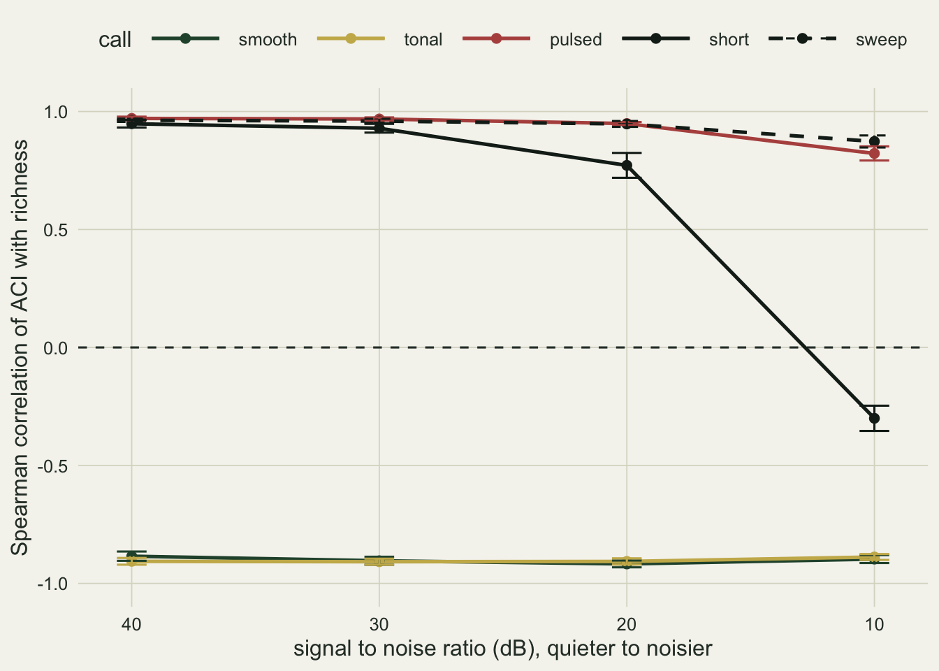
What to report
Report the noise conditions of each recording alongside any index, at minimum a background level per site, and show the index to richness relation separately for quiet and noisy recordings before pooling them. In the chorus simulation the same communities gave correlations of opposite sign at 40 dB and at 10 dB. Pooled across a road gradient, the noise level itself would dominate H, because noisy recordings sit near its maximum.
Report call activity, not just richness. If the ground truth is a point count, the number of detections or singing minutes is usually in the same notebook. The contrast between the two designs shows that the sign flip comes from call energy relative to the floor, so an index that correlates with richness in the field may be correlating with how much the birds sang that morning.
For the ACI, report the temporal step and the frequency limits, because the per-step normalisation makes the value depend on both, and say which kinds of call dominate the recordings. Whether the ACI rises or falls with richness depends on how long the calls stay in one frequency bin compared with the frame length: here notes that held a bin for 5 frames or fewer were rougher than the background, and a two frame note changed the sign of its correlation as the floor rose.
Treat a correlation between an index and richness as a property of the site set, not of the index. The meta-analysis by Alcocer and colleagues 2022 found a moderate mean correlation with large variation within and among studies, which is what these simulations would predict from differences in noise, activity and call type alone.
Honest limits
The spectrogram is built directly, with no waveform, no windowing and no leakage between bins. Signal and noise are added in power, which ignores phase; the frame envelope replaces the Hilbert envelope in Ht; and each species owns a clean band, so there is no masking or overlap. Real communities share bands, and overlap reduces how much Hf can gain from extra species; nothing here measures by how much.
The wind profile is a power law in frequency with a fixed exponent, stationary in time. Real wind and traffic are gusty, and a noise source that comes and goes changes Ht and the ACI in ways a stationary floor does not.
Richness is uniform on 1 to 21 and the amplitude distribution is the same at every site. Along a real gradient, distance to the microphone, vegetation and the identity of the loudest species all change together with richness. The simulations separate those on purpose; field data cannot.
Only H and the ACI are computed. The normalised difference soundscape index, the bioacoustic index and the acoustic diversity and evenness indices are also in common use and rest on different summaries (band ratios, areas under the spectrum, occupancy of frequency bands above a threshold). Nothing here says how they behave, although any index built on shares of energy will meet the same dependence on the floor.
The ACI implementation follows the verbal definition of Pieretti and colleagues 2011 on a linear magnitude matrix. Software implementations differ in whether they use magnitudes or decibels, in how the temporal step is set and in frequency limits, and the sign result for smooth calls rests on linear magnitudes of a stationary Rayleigh background. The dwell threshold is counted in frames, so it moves with the frame length and overlap of the transform; the short note and the sweep were added after the first results, and only these five templates were tried.
References
Sueur J, Pavoine S, Hamerlynck O, Duvail S 2008 PLoS ONE 3(12):e4065 (10.1371/journal.pone.0004065)
Pieretti N, Farina A, Morri D 2011 Ecological Indicators 11(3):868-873 (10.1016/j.ecolind.2010.11.005)
Alcocer I, Lima H, Sugai LSM, Llusia D 2022 Biological Reviews 97(6):2209-2236 (10.1111/brv.12890)