library(ggplot2)
options(scipen = 6)

te_paper  <- "#f5f4ee"
te_ink    <- "#16241d"
te_body   <- "#2c3a31"
te_forest <- "#275139"
te_rust   <- "#b5534e"
te_gold   <- "#c9b458"
te_line   <- "#dad9ca"

theme_datasheet <- function() {
  theme_minimal(base_size = 12) +
    theme(plot.background  = element_rect(fill = te_paper, colour = NA),
          panel.background = element_rect(fill = te_paper, colour = NA),
          panel.grid.major = element_line(colour = te_line, linewidth = 0.3),
          panel.grid.minor = element_blank(),
          text             = element_text(colour = te_body),
          axis.text        = element_text(colour = te_body),
          strip.text       = element_text(colour = te_ink, face = "bold"))
}Maximum likelihood by hand with optim() in R
R
maximum likelihood
GLM
nonlinear regression
count data
statistics
ecology tutorial
Write a negative log-likelihood in R, minimise it with optim(), match glm() to four decimals, avoid the product that underflows, then fit a curve glm() cannot.
Eighty quadrats across a wet meadow, half of them inside a cattle paddock, and in each one a count of marsh marigold plants and a reading of soil moisture. You already know how to fit this: glm(count ~ moisture + grazed, family = poisson). Then you open an occupancy or capture-recapture post on this site and find no glm() at all. Instead there is a function called nll, a vector of starting numbers, and a call to optim(). This post is the bridge between the two. It writes the likelihood that glm() maximises for you, maximises it by hand, and then uses the same recipe for a model that glm() cannot fit.
The recipe has four parts: a function that takes a vector of parameters and returns minus the log-likelihood of the data, a starting vector, a call to optim() that returns the minimum, and the curvature at that minimum, which gives the standard errors. Everything else in this post is a check that the recipe did what you think it did, and one trap that makes it fail before it takes a single step. Chapters 6 and 7 of Bolker (2008) teach the same recipe at book length, and the optim() help page documents every argument used below.
The short answer. Write the log-likelihood as a sum of log = TRUE densities, never as the log of a product. Return it with a minus sign, because optim() minimises. Ask for hessian = TRUE and invert the Hessian for the covariance. Keep each parameter on a scale where any real number is allowed (logs for positive quantities), and back-transform interval endpoints, not standard errors. Before you trust the recipe on a new model, run it once on a model that glm() can fit and compare.
The applied version of this recipe, for occupancy, is in Fitting single-season occupancy models in R. The data here are simulated, and every seed is in the code.
The meadow data
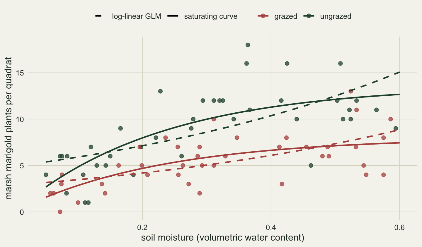
Soil moisture is recorded as volumetric water content, a fraction between 0.05 and 0.60. The true mean count rises with moisture and levels off in wet soil, and grazing lowers the level it reaches. The design constants are fixed in the code: an ungrazed asymptote of 12 plants per quadrat, a rate of 6 per unit of water content, and grazed quadrats reaching 0.6 of the ungrazed asymptote.
set.seed(1410)
n_quad   <- 80
moisture <- round(runif(n_quad, 0.05, 0.60), 3)     # volumetric water content
grazed   <- rep(c(0, 1), each = n_quad / 2)          # 1 = inside the paddock
a_true <- 12; b_true <- 6; graze_ratio <- 0.6        # design constants
lambda_true <- a_true * graze_ratio^grazed * (1 - exp(-b_true * moisture))

quads <- data.frame(moisture, grazed, count = rpois(n_quad, lambda_true))
head(quads, 3)
moisture grazed count
1 0.198 0 7
2 0.342 0 10
3 0.564 0 11A likelihood glm() already knows
A Poisson GLM with a log link says that each count is a Poisson draw whose mean is exp(b0 + b1 * moisture + b2 * grazed). The likelihood of the whole data set is the product of the 80 Poisson probabilities, one per quadrat, and its log is their sum. dpois(..., log = TRUE) gives each log probability directly. optim() looks for a minimum, so the function returns the sum with a minus sign. The default search in optim() is Nelder-Mead, which only compares function values; method = "BFGS" also uses the slope of the function, and it is the usual choice for a smooth likelihood with a few parameters:
nll_pois <- function(par, dat) {
  eta <- par[1] + par[2] * dat$moisture + par[3] * dat$grazed
  -sum(dpois(dat$count, lambda = exp(eta), log = TRUE))
}
fit_hand <- optim(c(0, 0, 0), nll_pois, dat = quads, method = "BFGS", hessian = TRUE)
fit_glm  <- glm(count ~ moisture + grazed, family = poisson, data = quads)
se_hand <- sqrt(diag(solve(fit_hand$hessian)))
compare <- data.frame(optim = fit_hand$par, glm = coef(fit_glm),
                      se_optim = se_hand, se_glm = sqrt(diag(vcov(fit_glm))))
round(compare, 4)
optim glm se_optim se_glm
(Intercept) 1.5894 1.5894 0.1030 0.1030
moisture 1.8729 1.8729 0.2569 0.2569
grazed -0.5318 -0.5318 0.0860 0.0860Both columns agree to the four decimals printed, estimates and standard errors alike: the largest difference is \(2.0 \times 10^{-6}\) for an estimate and \(1.4 \times 10^{-6}\) for a standard error, the size of difference left by the stopping rule of the search and by the numerical second derivatives. The minimum value of the function, 191.4158, is minus the log-likelihood that logLik(fit_glm) reports. (If you prefer to maximise, control = list(fnscale = -1) makes optim() do that, and then the function returns the log-likelihood without the minus sign.)
The standard errors come from the Hessian, the matrix of second derivatives of the function at its minimum, which optim() estimates numerically when asked. A sharply curved minimum means the data pin the parameter down; a flat one means they do not. Inverting the Hessian of minus the log-likelihood gives the estimated covariance matrix of the parameters, and the square roots of its diagonal are the standard errors. glm() uses the expected curvature, averaged over the data the model could produce, instead of the curvature of this data set’s function, and for a Poisson model with a log link or a binomial model with a logit link the two are the same, which is why the columns match. With other links the two can differ, and families such as gaussian or Gamma add a dispersion parameter that glm() estimates by a route of its own, so run the comparison on one of those two models.
Moisture is stored as a fraction on purpose. With the same readings in per cent, the moisture coefficient is a hundred times smaller (0.0187 instead of 1.87), and the same optim() call stops 0.0010 away from the glm() intercept. That is harmless here, less than a hundredth of the intercept’s standard error of 0.103, but it is 473 times the largest gap left with moisture as a fraction. Why a parameter’s size changes what optim() finds, and what to do about it, is the subject of Parameter scale decides what optim() finds.
The product that turns into zero
The likelihood is a product, so it is tempting to write it as one and take the log at the end. On these data, from the same starting values, that version cannot even begin:
nll_prod <- function(par, dat) {
  eta <- par[1] + par[2] * dat$moisture + par[3] * dat$grazed
  -log(prod(dpois(dat$count, lambda = exp(eta))))
}
nll_prod(c(0, 0, 0), quads)
[1] Inffit_prod <- tryCatch(optim(c(0, 0, 0), nll_prod, dat = quads, method = "BFGS"),
error = function(e) e)
conditionMessage(fit_prod)[1] "initial value in 'vmmin' is not finite"running <- cumprod(dpois(quads$count, lambda = 1)) # the start: every mean is exp(0) = 1
first_tiny <- which(running < .Machine$double.xmin)[1]
first_zero <- which(running == 0)[1]
c(below_double_xmin = first_tiny, exactly_zero = first_zero)below_double_xmin exactly_zero
55 60 At the start every quadrat is given a mean of one plant, so a quadrat with ten plants has a Poisson probability of \(1.0 \times 10^{-7}\), and the running product shrinks fast. R stores numbers as doubles. Below .Machine$double.xmin, which is 2^-1022 or \(2.2 \times 10^{-308}\), a double keeps fewer and fewer digits, and below 2^-1074 (\(4.9 \times 10^{-324}\)) no positive number is left. Multiplying the probabilities in row order, the product passes the first of these lines at quadrat 55 and reaches exactly zero at quadrat 60. The log of zero is -Inf, minus that is Inf, and optim() stops with an error before its first step. The sum of logs has no such floor: dpois(200, 1) is zero in R, while dpois(200, 1, log = TRUE) is -864.2.
On these 80 quadrats a sensible start rescues it. With the log of the mean count as the intercept and zeros for the two slopes, the product version returns a finite 234.61 and BFGS reaches the glm() answer; at the maximum the product of the 80 probabilities is \(7.4 \times 10^{-84}\), far from the floor. For a larger survey, though, even the right answer underflows. Here is the same design with 1000 quadrats, with every probability computed at the TRUE parameter values:
set.seed(1411)
big_moist  <- runif(1000, 0.05, 0.60)
big_grazed <- rep(c(0, 1), 500)
big_lambda <- a_true * graze_ratio^big_grazed * (1 - exp(-b_true * big_moist))
big_count  <- rpois(1000, big_lambda)
big_logp   <- dpois(big_count, big_lambda, log = TRUE)
big_zero   <- which(cumprod(dpois(big_count, big_lambda)) == 0)[1]
big_zero                        # the product, in row order, is zero from here on
[1] 308sum(big_logp) # the sum of logs is an ordinary number[1] -2420.459log(2^-1074) / mean(big_logp) # how many average quadrats reach the floor[1] 307.5615With the true values plugged in, the product is zero from quadrat 308 onwards, while the sum of logs, -2420.5, is an ordinary number. The quadrat where it happens follows from two numbers. The log of the smallest positive double is log(2^-1074), or -744.4, and at the true values an average quadrat adds -2.42 to the log-likelihood, so the product runs out after about 744.4 / 2.42 = 308 quadrats. A survey of that size is not unusual, and the product version then has nothing to work with even at the right answer. Use the sum.
A curve glm() cannot fit
The log-linear GLM makes the mean grow exponentially with moisture, without limit. The simulated meadow does something else: the count is low in dry soil, rises as the soil gets wetter, and above some moisture it levels off. A curve with those three properties is lambda = a * exp(g * grazed) * (1 - exp(-b * moisture)), where a is the ungrazed asymptote, b is how quickly the count approaches it, and exp(g) is the grazed asymptote as a share of the ungrazed one. The rate b sits inside an exponential inside the mean, and no link function turns this mean into coefficients times columns of data, which is the form every glm() needs. For optim() it is only a different line inside the function.
a and b must be positive. Instead of constraining the search, the function takes their logs and exponentiates them, so any real number is a legal value:
nll_sat <- function(par, dat) {
  a <- exp(par[1]); b <- exp(par[2]); g <- par[3]
  lambda <- a * exp(g * dat$grazed) * (1 - exp(-b * dat$moisture))
  -sum(dpois(dat$count, lambda, log = TRUE))
}
init_sat <- c(log(10), log(5), 0)     # read off the scatter: level near 10, most of the rise done by 0.3
fit_sat  <- optim(init_sat, nll_sat, dat = quads, method = "BFGS", hessian = TRUE)
se_sat   <- sqrt(diag(solve(fit_sat$hessian)))
z95 <- qnorm(0.975)
sat_table <- data.frame(estimate = exp(fit_sat$par),
                        lower = exp(fit_sat$par - z95 * se_sat),
                        upper = exp(fit_sat$par + z95 * se_sat),
                        row.names = c("a (ungrazed asymptote)", "b (rate)", "exp(g) (grazed share)"))
round(sat_table, 3)
estimate lower upper
a (ungrazed asymptote) 13.656 10.931 17.060
b (rate) 4.381 2.846 6.744
exp(g) (grazed share) 0.588 0.497 0.696Each interval is built on the scale where the search ran and then its two endpoints are exponentiated. The asymptote comes out at 13.66 plants per quadrat with an interval from 10.93 to 17.06, which reaches further above the estimate than below it, as an interval built on the log scale does. Grazed quadrats level off at 0.59 of the ungrazed asymptote (interval 0.50 to 0.70). The standard error 0.114 belongs to log a; it is not a standard error of a in plants, and an interval of 13.66 plus or minus 1.96 times it would be 0.45 plants wide instead of 6.13. A second start far from the first, at a = 20, b = 1 and g = -1, reaches the same minimum; Starting values and identifiability in nls covers choosing starts, and the case where no start can pin a parameter down.
Nested models: likelihood ratio and AIC
Does grazing lower the asymptote? Fix g at zero, fit again, and compare. The two fits are nested (the smaller one is the larger one with a parameter held at a value inside its range), so twice the difference in their log-likelihoods has, in large samples, a chi-squared distribution with one degree of freedom when grazing does nothing (Wilks 1938). The minimum values from optim() are all the test needs:
nll_sat_nograze <- function(par, dat) nll_sat(c(par, 0), dat)
fit_nograze <- optim(fit_sat$par[1:2], nll_sat_nograze, dat = quads, method = "BFGS")
lr_stat <- 2 * (fit_nograze$value - fit_sat$value)
round(c(LR = lr_stat, critical_95 = qchisq(0.95, df = 1)), 2)
LR critical_95
39.40 3.84 formatC(pchisq(lr_stat, df = 1, lower.tail = FALSE), format = "e", digits = 1) # p-value[1] "3.5e-10"AIC comes from the same numbers: twice the minimum plus twice the number of parameters. It also compares the saturating curve with the log-linear GLM, which the likelihood ratio test cannot do, because neither of those two models is a special case of the other. The comparison is fair because both functions use the full Poisson density, constants included:
aic_tab <- c(loglinear_glm      = 2 * fit_hand$value + 2 * 3,
             saturating_nograze = 2 * fit_nograze$value + 2 * 2,
             saturating_grazed  = 2 * fit_sat$value + 2 * 3)
round(aic_tab - min(aic_tab), 2)
loglinear_glm saturating_nograze saturating_grazed
17.17 37.40 0.00 The likelihood ratio statistic is 39.4 against a 95 per cent critical value of 3.84 (p = \(3.5 \times 10^{-10}\)), so the grazing term stays. The hand-computed AIC of the log-linear model equals AIC(fit_glm), 388.83, and the saturating curve with grazing is lower by 17.2. What an AIC difference of that size means, and when to average over models instead of choosing one, is in Model selection with AIC in R for ecology.
Profile likelihood next to the Wald interval
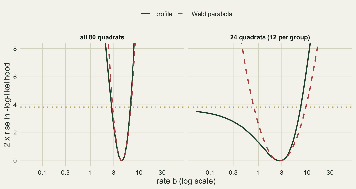
The intervals above are Wald intervals: estimate plus or minus 1.96 standard errors, on the log scale. They treat minus the log-likelihood as a parabola around its minimum, with the curvature measured at the bottom. A profile likelihood interval uses the function itself instead. Fix b at a value, let optim() find the best a and g for it, and record the minimum; repeat along a grid of b. Twice the rise of that profile above the overall minimum is the likelihood ratio statistic of the previous section for that value of b, so it is compared with qchisq(0.95, 1), and the interval is the set of b values below that cut (Venzon and Moolgavkar 1988):
profile_b <- function(log_b, dat, init) {
  inner <- function(p) nll_sat(c(p[1], log_b, p[2]), dat)   # p = (log a, g)
  optim(init, inner, method = "BFGS")$value
}
grid_lb <- seq(log(0.05), log(60), length.out = 500)   # b from 0.05 to 60, even steps on the log scale
cut_95  <- qchisq(0.95, 1)
wald_b  <- function(fit) exp(fit$par[2] + c(-1, 1) * z95 * sqrt(diag(solve(fit$hessian)))[2])

dev_all <- 2 * (sapply(grid_lb, profile_b, dat = quads, init = fit_sat$par[c(1, 3)]) - fit_sat$value)
small <- quads[c(1:12, 41:52), ]      # 24 quadrats: the first 12 of each group
fit_small <- optim(init_sat, nll_sat, dat = small, method = "BFGS", hessian = TRUE)
dev_small <- 2 * (sapply(grid_lb, profile_b, dat = small, init = fit_small$par[c(1, 3)]) - fit_small$value)

ci_tab <- rbind(profile_80 = range(exp(grid_lb[dev_all < cut_95])),   wald_80 = wald_b(fit_sat),
                profile_24 = range(exp(grid_lb[dev_small < cut_95])), wald_24 = wald_b(fit_small))
colnames(ci_tab) <- c("lower", "upper")
round(ci_tab, 2)
lower upper
profile_80 2.71 6.54
wald_80 2.85 6.74
profile_24 0.05 7.33
wald_24 0.80 9.46range() takes the smallest and the largest b on the grid whose profile lies below the cut, so the ends are only as fine as the grid: neighbouring grid points are 1.4 per cent apart. It also assumes a single valley, which the figure below shows. When an end of the interval lands on the first or last point of the grid, the grid was too narrow on that side: widen it and look again. If the end stays on the edge however far you widen, the interval has no end on that side.
With all 80 quadrats the two intervals for b are close: the profile runs from 2.71 to 6.54 and the Wald interval from 2.85 to 6.74. With 24 quadrats they are not. The estimate is 2.75 and the Wald interval is 0.80 to 9.46. The profile interval ends at 7.33 on the right, but its lower end in the table, 0.05, is the first point of the grid, not an end of the interval. As b shrinks, the best a grows so that a * b settles at a fixed value, and the curve becomes a straight line through the origin in each group. For that straight line, twice the rise in minus the log-likelihood is 3.67, below the cut of 3.84, so the profile never reaches the cut on that side and the interval has no lower end above zero. The 24 quadrats cannot rule out that the count never levels off in this moisture range, and only the profile says so.
The profile costs one optim() call per grid point, which is cheap for three parameters. For other ways of putting an interval on a derived quantity (the delta method, Fieller’s interval) see Confidence intervals for effective doses; for what a confidence interval promises in the first place, Standard errors and confidence intervals in R.
What to check in your own data
Before you trust a hand-written likelihood, run the same code on a model glm() can fit, and compare estimates, logLik() and, for a Poisson log-link or binomial logit-link model, the standard errors. If they disagree, the bug is in your function, not in the new model.
Evaluate the function at your starting values before calling optim(). It must return a finite number. If it returns Inf or NaN, look for a product of densities, a log() of something that can be zero, or a parameter that has left its allowed range.
Look at fit$convergence (zero means the search stopped normally, not that it found the right answer) and run it again from a clearly different start. Two starts that end at the same minimum value are the cheapest check you have.
Report intervals for positive or bounded parameters by transforming the endpoints of an interval built on the search scale. When the sample is small or an estimate sits near a limit of its range, compute a profile interval for the parameter you care about and report it if it disagrees with the Wald interval.
Honest limits
The demonstration assumes the counts are Poisson, which the simulation makes true; with real quadrat counts, check for overdispersion before trusting any of the standard errors above. The Hessian here is a finite-difference estimate, and its standard errors agreed with glm() to within \(1.4 \times 10^{-6}\) in this example; for badly scaled or nearly flat problems it can be much worse, or not invertible at all. The chi-squared reference for the likelihood ratio test needs the null value to sit inside the parameter range: testing whether a variance is zero, or whether a mixture needs a second component, puts it on the edge, and the test then needs a different reference distribution. The comparison of profile and Wald intervals uses one simulated data set and 24 of its quadrats (the first 12 of each group); it shows that the two can disagree, not how often either one covers the true value, which would need a simulation of its own.
References
Bolker BM 2008 Ecological Models and Data in R (ISBN 978-0-691-12522-0)
R Core Team 2024 R documentation: General-purpose optimization, optim (https://stat.ethz.ch/R-manual/R-devel/library/stats/html/optim.html)
Venzon DJ, Moolgavkar SH 1988 Applied Statistics 37(1):87-94 (10.2307/2347496)
Wilks SS 1938 The Annals of Mathematical Statistics 9(1):60-62 (10.1214/aoms/1177732360)