Confidence intervals for effective doses

Delta, Fieller and profile intervals for the LC50 and LC10 in R, with measured coverage, and why the concentration layout matters more than the animal count.

A contract laboratory finishes an acute immobilisation test on a freshwater invertebrate. Six concentrations, 25 animals in each, immobilised animals counted at the end, one binomial curve fitted through the six proportions. The report gives an LC50 with a 95 per cent confidence interval, the client files it, and nobody looks at the interval again. Then the risk assessment comes back with a different request: the concentration that immobilises one animal in ten, with a lower confidence limit on it, because the threshold that goes into the assessment has to be one the substance is unlikely to exceed. Same test, same 150 animals, same fitted curve. The interval that came out of the fit for the LC50 was a little over two-fold wide. The one for the LC10 is nearly six-fold wide, and the one for the LC1 is more than thirty-fold.

That is the subject here. An effective dose is a quantile read backwards off a fitted curve, so its interval is an interval for a ratio of two estimated coefficients, and ratios are where symmetric intervals stop working. This tutorial fits the curve with a hand written Newton solver, puts three intervals on the same fitted quantile (delta method, Fieller’s theorem, profile likelihood), measures what each of them actually covers over 4000 simulated tests, and then asks the question that decides the answer: given a fixed number of animals, where should the concentrations go?

Dose-response curves and the LC50 built the point estimate and measured what the choice of link function does to it; everything below takes the link as given and works on the uncertainty. Return levels and uncertainty runs the same tail logic in extreme value analysis, where the interval for a rare flood widens and skews for the reason a low effective dose does. The design half of the post is a special case of what power analysis by simulation does for a difference between groups.

library(ggplot2)

te_pal <- list(forest = "#275139", green = "#2f8f63", sage = "#93a87f",
               clay = "#b5534e", gold = "#cda23f", line = "#dad9ca",
               ink = "#16241d", paper = "#f5f4ee")

theme_te <- function() {
  theme_minimal(base_size = 12) +
    theme(panel.grid.minor = element_blank(),
          panel.grid.major = element_line(colour = "#e7e6dc"),
          plot.background = element_rect(fill = "#f5f4ee", colour = NA),
          panel.background = element_rect(fill = "#f5f4ee", colour = NA),
          plot.title = element_text(face = "bold", colour = te_pal$ink),
          axis.title = element_text(colour = "#2c3a31"))
}

A standard acute test and the number it produces

The generating curve is log-logistic: the probability of a response at concentration \(d\) is \(1 / (1 + \exp(-b(\log_{10} d - \log_{10} \mathrm{LC}_{50})))\), with a true LC50 of 12 micrograms per litre and a slope of 2.4 per decade. Written that way it is a binomial generalised linear model with a logit link and \(\log_{10} d\) as the only predictor, which is the machinery of logistic regression for presence-absence data pointed at a different question: not what the predictor does, but where a chosen quantile of the fitted curve sits. The same log-logistic distribution appears in parametric survival and the AFT model, where it describes a time to event; here it describes a proportion running along a concentration axis, and nothing below depends on time.

The design is the standard factor-of-two ladder: 2, 4, 8, 16, 32 and 64 micrograms per litre, 25 animals at each, 150 in total.

lc50_true  <- 12
slope_true <- 2.4
x50_true   <- log10(lc50_true)

lx_true <- function(lev) x50_true + qlogis(lev) / slope_true
lc_true <- function(lev) 10^lx_true(lev)

conc_wide <- c(2, 4, 8, 16, 32, 64)
n_wide    <- rep(25, 6)
x_wide    <- log10(conc_wide)
p_wide    <- 1 / (1 + exp(-slope_true * (x_wide - x50_true)))

print(data.frame(concentration = conc_wide, animals = n_wide,
                 log10_conc = round(x_wide, 4),
                 true_response = round(p_wide, 4)))

  concentration animals log10_conc true_response
1             2      25     0.3010        0.1338
2             4      25     0.6021        0.2414
3             8      25     0.9031        0.3959
4            16      25     1.2041        0.5744
5            32      25     1.5051        0.7354
6            64      25     1.8062        0.8513

levs <- c(0.5, 0.1, 0.01)
print(round(rbind(level = levs, true_dose = lc_true(levs),
                  true_log10_dose = lx_true(levs)), 4))

                   [,1]   [,2]    [,3]
level            0.5000 0.1000  0.0100
true_dose       12.0000 1.4577  0.1461
true_log10_dose  1.0792 0.1637 -0.8355

c(true_lc50 = lc50_true, true_slope_per_decade = slope_true,
  total_animals = sum(n_wide),
  doses_below_the_true_lc10 = sum(conc_wide < lc_true(0.1)),
  animals_below_the_true_lc10 = sum(n_wide[conc_wide < lc_true(0.1)]))

                  true_lc50       true_slope_per_decade 
                       12.0                         2.4 
              total_animals   doses_below_the_true_lc10 
                      150.0                         0.0 
animals_below_the_true_lc10 
                        0.0 

The true LC50 of 12 sits between the fourth and fifth rungs of the ladder, where a well placed test wants it. The true LC10 is 1.4577 and the true LC1 is 0.1461, and this is the fact the whole post turns on: the lowest concentration tested is 2, which is above the true LC10, so 0 of the 6 concentrations and 0 of the 150 animals lie below the response level the risk assessment cares about. The LC10 is an extrapolation, and the LC1 is an extrapolation by more than a factor of ten below the lowest treatment.

Three intervals for the same fitted quantile

The fitting code below is written by hand rather than called from glm, because everything after this section refits the same model thousands of times and a vectorised Newton solver does all the replicates in one set of matrix operations. The step is damped by dividing it by \(1 + |step| / 0.5\), which leaves Newton’s step alone when it is small and shrinks it when it is large. Without that damping the solver can fall into a two point cycle on data sets where the slope is weakly determined, which is the sort of failure that quietly poisons a coverage study.

log1pexp <- function(e) ifelse(e > 30, e, log1p(exp(e)))

fit_many <- function(x, n_an, Y) {
  k <- length(x); nrep <- ncol(Y)
  bb <- rbind(rep(0, nrep), rep(1, nrep))
  for (it in 1:60) {
    eta <- x %o% bb[2, ] + rep(bb[1, ], each = k)
    pr <- 1 / (1 + exp(-eta))
    wt <- n_an * pr * (1 - pr); wt[wt < 1e-10] <- 1e-10
    res <- Y - n_an * pr
    s1 <- colSums(res); s2 <- colSums(x * res)
    h11 <- colSums(wt); h12 <- colSums(x * wt); h22 <- colSums(x * x * wt)
    det2 <- h11 * h22 - h12^2
    d1 <- (h22 * s1 - h12 * s2) / det2
    d2 <- (-h12 * s1 + h11 * s2) / det2
    big <- pmax(abs(d1), abs(d2))
    damp <- 1 / (1 + big / 0.5)
    bb[1, ] <- bb[1, ] + damp * d1
    bb[2, ] <- bb[2, ] + damp * d2
    if (max(damp * big) < 1e-11) break
  }
  eta <- x %o% bb[2, ] + rep(bb[1, ], each = k)
  pr <- 1 / (1 + exp(-eta))
  list(b0 = bb[1, ], b1 = bb[2, ], v00 = h22 / det2, v01 = -h12 / det2,
       v11 = h11 / det2, loglik = colSums(Y * eta - n_an * log1pexp(eta)),
       iterations = it, last_step = max(big))
}

simulate_counts <- function(x, n_an, nrep, x50 = x50_true, slope = slope_true) {
  pr <- 1 / (1 + exp(-slope * (x - x50)))
  matrix(rbinom(length(x) * nrep, rep(n_an, nrep), rep(pr, nrep)), length(x), nrep)
}

One simulated test, fitted both ways, checks the solver before anything is built on it.

set.seed(20260730)
y_ex <- simulate_counts(x_wide, n_wide, 1)
print(data.frame(concentration = conc_wide, animals = n_wide,
                 dead = as.vector(y_ex),
                 observed = round(as.vector(y_ex) / n_wide, 4)))

  concentration animals dead observed
1             2      25    3     0.12
2             4      25    7     0.28
3             8      25   12     0.48
4            16      25   19     0.76
5            32      25   15     0.60
6            64      25   21     0.84

fit_ex <- fit_many(x_wide, n_wide, y_ex)
ref <- glm(cbind(as.vector(y_ex), n_wide - as.vector(y_ex)) ~ x_wide,
           family = binomial)
print(round(rbind(newton = c(fit_ex$b0, fit_ex$b1),
                  glm = as.numeric(coef(ref))), 6))

            [,1]     [,2]
newton -2.187769 2.141719
glm    -2.187769 2.141719

round(c(max_coefficient_difference = max(abs(c(fit_ex$b0, fit_ex$b1) -
                                                as.numeric(coef(ref)))),
        max_variance_difference =
          max(abs(c(fit_ex$v00, fit_ex$v01, fit_ex$v11) -
                    as.numeric(vcov(ref))[c(1, 2, 4)])),
        newton_iterations = fit_ex$iterations), 10)

max_coefficient_difference    max_variance_difference 
                   0.0e+00                    9.6e-09 
         newton_iterations 
                   1.2e+01 

est_ex <- (qlogis(levs) - fit_ex$b0) / fit_ex$b1
print(round(rbind(level = levs, estimate = 10^est_ex, truth = lc_true(levs)), 4))

            [,1]   [,2]   [,3]
level     0.5000 0.1000 0.0100
estimate 10.5076 0.9899 0.0752
truth    12.0000 1.4577 0.1461

The two fits give the same intercept of -2.187769 and the same slope of 2.141719, with a largest coefficient difference of 0 and variance entries agreeing to nine decimal places. On this data set the fitted LC50 is 10.5076 against a true 12, an error that no reviewer would blink at. The fitted LC10 is 0.9899 against a true 1.4577, which is out by a third, and the fitted LC1 is 0.0752 against 0.1461, out by nearly a half. Nothing went wrong. The same two coefficients produce all three, and the error grows as you walk down the curve because the estimated slope enters the extrapolation multiplied by how far you are walking.

Three recipes turn that estimate into an interval. Write \(L_q\) for the logit of the target response level and \(x_q = (L_q - b_0) / b_1\) for the estimate on the \(\log_{10}\) concentration scale.

The delta method treats \(x_q\) as approximately normal, takes its variance from a first order expansion of the ratio, and puts the interval at plus and minus 1.96 standard errors. Carried out on the log concentration scale it is symmetric in \(\log_{10} d\) and multiplicative in \(d\), which is already an improvement on the version some reporting templates still use, the same expansion carried out on the raw concentration scale. Both are computed below.

Fieller’s theorem refuses to linearise. The event \(b_0 + b_1 x = L_q\) is linear in the coefficients, so \(b_0 + b_1 x - L_q\) is normal with a variance that is a quadratic in \(x\), and the set of \(x\) values the data cannot reject at the 5 per cent level is the solution of a quadratic inequality. When the leading coefficient \(b_1^2 - z^2 v_{11}\) is not positive, meaning the slope itself is not distinguishable from zero, the solution set is not a bounded interval and Fieller says so instead of pretending otherwise.

Profile likelihood reparametrises the model so that the effective dose is a parameter. Fix \(x_q\), write the linear predictor as \(L_q + b(x - x_q)\), maximise over the single remaining parameter \(b\), and keep every \(x_q\) whose maximised log-likelihood is within half a chi-squared quantile of the overall maximum. The bounds are found by bisection, vectorised so that every replicate advances together.

rep_fit <- function(fit, times) {
  lapply(fit[c("b0", "b1", "v00", "v01", "v11", "loglik")], rep, times = times)
}

delta_log <- function(lev, fit) {
  xq <- (qlogis(lev) - fit$b0) / fit$b1
  vv <- (fit$v00 + 2 * xq * fit$v01 + xq^2 * fit$v11) / fit$b1^2
  se <- sqrt(pmax(vv, 0))
  cbind(xq - qnorm(0.975) * se, xq + qnorm(0.975) * se)
}

delta_dose <- function(lev, fit) {
  xq <- (qlogis(lev) - fit$b0) / fit$b1
  vv <- (fit$v00 + 2 * xq * fit$v01 + xq^2 * fit$v11) / fit$b1^2
  se <- sqrt(pmax(vv, 0)) * log(10) * 10^xq
  cbind(10^xq - qnorm(0.975) * se, 10^xq + qnorm(0.975) * se)
}

fieller_log <- function(lev, fit) {
  z2 <- qnorm(0.975)^2
  aa <- fit$b1^2 - z2 * fit$v11
  gap <- fit$b0 - qlogis(lev)
  bq <- 2 * (gap * fit$b1 - z2 * fit$v01)
  cq <- gap^2 - z2 * fit$v00
  disc <- bq^2 - 4 * aa * cq
  lo <- rep(-Inf, length(aa)); hi <- rep(Inf, length(aa))
  ok <- aa > 0 & disc > 0
  r1 <- (-bq - sqrt(pmax(disc, 0))) / (2 * aa)
  r2 <- (-bq + sqrt(pmax(disc, 0))) / (2 * aa)
  lo[ok] <- pmin(r1, r2)[ok]; hi[ok] <- pmax(r1, r2)[ok]
  cbind(lo, hi)
}

profile_loglik <- function(xq, lq, x, n_an, Y, b_start) {
  k <- length(x)
  uu <- outer(x, xq, "-")
  bb <- b_start
  for (it in 1:80) {
    eta <- rep(lq, each = k) + uu * rep(bb, each = k)
    pr <- 1 / (1 + exp(-eta))
    sc <- colSums(uu * (Y - n_an * pr))
    hs <- colSums(n_an * pr * (1 - pr) * uu^2); hs[hs < 1e-10] <- 1e-10
    st <- sc / hs
    st <- st / (1 + abs(st) / 0.5)
    bb <- bb + st
    if (max(abs(st)) < 1e-11) break
  }
  eta <- rep(lq, each = k) + uu * rep(bb, each = k)
  colSums(Y * eta - n_an * log1pexp(eta))
}

profile_log <- function(lev, x, n_an, Y, fit, span = 14, steps = 46) {
  lq <- qlogis(lev)
  xhat <- (lq - fit$b0) / fit$b1
  crit <- fit$loglik - qchisq(0.95, 1) / 2
  out <- matrix(NA_real_, length(xhat), 2)
  for (side in c(-1, 1)) {
    far <- xhat + side * span
    unbounded <- profile_loglik(far, lq, x, n_an, Y, fit$b1) > crit
    lo <- xhat; hi <- far
    for (it in 1:steps) {
      mid <- (lo + hi) / 2
      inside <- profile_loglik(mid, lq, x, n_an, Y, fit$b1) > crit
      lo <- ifelse(inside, mid, lo)
      hi <- ifelse(inside, hi, mid)
    }
    bnd <- (lo + hi) / 2
    bnd[unbounded] <- side * Inf
    out[, if (side < 0) 1 else 2] <- bnd
  }
  out
}

cat("z for a two sided 95 per cent interval:", round(qnorm(0.975), 2),
    "| chi-squared quantile:", round(qchisq(0.95, 1), 4),
    "| nominal miss per side:", 0.025, "or in per cent:", 2.5,
    "| one sided level in per cent:", 97.5, "\n")

z for a two sided 95 per cent interval: 1.96 | chi-squared quantile: 3.8415 | nominal miss per side: 0.025 or in per cent: 2.5 | one sided level in per cent: 97.5 

nlev <- length(levs)
fit_rep <- rep_fit(fit_ex, nlev)
Y_rep <- matrix(rep(as.vector(y_ex), nlev), length(x_wide), nlev)
d_log <- delta_log(levs, fit_rep)
d_dose <- delta_dose(levs, fit_rep)
f_log <- fieller_log(levs, fit_rep)
p_log <- profile_log(levs, x_wide, n_wide, Y_rep, fit_rep)

ex_tab <- cbind(level = levs, estimate = 10^est_ex,
                delta_lo = 10^d_log[, 1], delta_hi = 10^d_log[, 2],
                fieller_lo = 10^f_log[, 1], fieller_hi = 10^f_log[, 2],
                profile_lo = 10^p_log[, 1], profile_hi = 10^p_log[, 2],
                dose_delta_lo = d_dose[, 1], dose_delta_hi = d_dose[, 2])
print(round(ex_tab, 4))

     level estimate delta_lo delta_hi fieller_lo fieller_hi profile_lo
[1,]  0.50  10.5076   7.1066  15.5362     6.8560    15.8934     6.9363
[2,]  0.10   0.9899   0.3774   2.5962     0.2265     2.0505     0.2498
[3,]  0.01   0.0752   0.0116   0.4866     0.0040     0.2981     0.0049
     profile_hi dose_delta_lo dose_delta_hi
[1,]    15.7383        6.3983       14.6168
[2,]     2.1107        0.0354        1.9443
[3,]     0.3149       -0.0652        0.2155

upper_over_lower <- function(bnd) (10^bnd[, 2] - 10^est_ex) / (10^est_ex - 10^bnd[, 1])
print(round(rbind(level = levs, delta = upper_over_lower(d_log),
                  fieller = upper_over_lower(f_log),
                  profile = upper_over_lower(p_log)), 4))

          [,1]   [,2]   [,3]
level   0.5000 0.1000 0.0100
delta   1.4786 2.6227 6.4742
fieller 1.4750 1.3893 3.1350
profile 1.4647 1.5145 3.4135

At the LC50 the three barely differ: 7.1066 to 15.5362 for the delta method, 6.8560 to 15.8934 for Fieller, 6.9363 to 15.7383 for the profile. At the LC10 they have parted company. The delta interval runs from 0.3774 to 2.5962, the profile from 0.2498 to 2.1107, Fieller from 0.2265 to 2.0505. The delta lower limit is more than half again as high as the other two, and it is the lower limit that a risk assessment uses. At the LC1 the delta lower limit of 0.0116 is more than twice the profile’s 0.0049.

The last table measures the shape. Divide the distance from the estimate up to the upper limit by the distance down to the lower limit, on the concentration scale where people read the number. At the LC50 all three land between 1.4647 and 1.4786, the mild right skew any multiplicative interval has. At the LC1 the delta method reports 6.4742 while the profile reports 3.4135 and Fieller 3.1350. The delta method is not producing a symmetric interval on the dose scale; it is producing a more lopsided one than either likelihood based method, and lopsided in the direction that shortens the lower arm.

The version on the raw concentration scale, in the last two columns of the first table, fails outright. Its LC1 interval runs from -0.0652 to 0.2155 micrograms per litre. A negative concentration is not a conservative bound, it is an empty statement.

lev_grid <- plogis(seq(qlogis(0.004), qlogis(0.95), length.out = 70))
fit_g <- rep_fit(fit_ex, length(lev_grid))
Y_g <- matrix(rep(as.vector(y_ex), length(lev_grid)), length(x_wide),
              length(lev_grid))
bnd <- list(Delta = delta_log(lev_grid, fit_g),
            Fieller = fieller_log(lev_grid, fit_g),
            Profile = profile_log(lev_grid, x_wide, n_wide, Y_g, fit_g))
c(non_finite_bounds_in_figure = sum(!is.finite(unlist(bnd))))

non_finite_bounds_in_figure 
                          0 

band <- do.call(rbind, lapply(names(bnd), function(nm)
  data.frame(lev = rep(lev_grid, 2), xx = as.vector(bnd[[nm]]),
             side = rep(c("lo", "hi"), each = length(lev_grid)), method = nm)))
band$method <- factor(band$method, levels = names(bnd))
curve_df <- data.frame(xx = seq(-2.6, 3, length.out = 240))
curve_df$fitted <- 1 / (1 + exp(-(fit_ex$b0 + fit_ex$b1 * curve_df$xx)))
curve_df$truth <- 1 / (1 + exp(-slope_true * (curve_df$xx - x50_true)))
obs_df <- data.frame(xx = x_wide, lev = as.vector(y_ex) / n_wide)
mark <- data.frame(lev = levs, lab = c("LC50", "LC10", "LC1"))
brk <- log10(c(0.01, 0.1, 1, 10, 100, 1000))

ggplot(band, aes(xx, lev, colour = method, group = interaction(method, side))) +
  geom_hline(data = mark, aes(yintercept = lev),
             colour = te_pal$line, linewidth = 0.8) +
  geom_line(data = curve_df, aes(xx, truth), inherit.aes = FALSE,
            colour = te_pal$ink, linetype = "dashed", linewidth = 0.7) +
  geom_line(data = curve_df, aes(xx, fitted), inherit.aes = FALSE,
            colour = te_pal$ink, linewidth = 0.9) +
  geom_line(linewidth = 0.85) +
  geom_point(data = obs_df, aes(xx, lev), inherit.aes = FALSE,
             colour = te_pal$ink, size = 2.4) +
  geom_text(data = mark, aes(x = -2.5, y = lev, label = lab), inherit.aes = FALSE,
            vjust = -0.5, hjust = 0, size = 3.1, colour = "#2c3a31") +
  scale_colour_manual(values = c(Delta = te_pal$clay, Fieller = te_pal$green,
                                 Profile = te_pal$gold), name = NULL) +
  scale_x_continuous(breaks = brk,
                     labels = c("0.01", "0.1", "1", "10", "100", "1000")) +
  scale_y_continuous(trans = "logit",
                     breaks = c(0.01, 0.05, 0.1, 0.25, 0.5, 0.75, 0.9),
                     labels = c("0.01", "0.05", "0.10", "0.25", "0.50",
                                "0.75", "0.90")) +
  coord_cartesian(xlim = c(-2.6, 3), ylim = c(0.006, 0.93)) +
  labs(x = "Concentration (micrograms per litre, log scale)",
       y = "Proportion responding",
       title = "The interval on the concentration axis opens out as the level falls",
       subtitle = "Solid black: the fitted curve. Dashed black: the curve the counts were generated from.") +
  theme_te() +
  theme(legend.position = "right",
        plot.subtitle = element_text(colour = "#2c3a31", size = 9))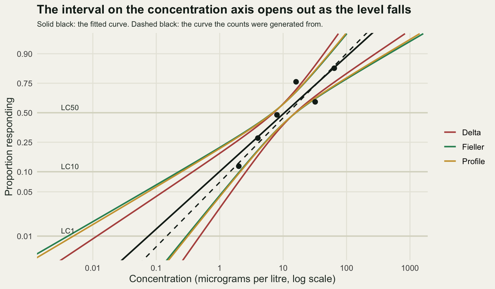

Figure 1: One simulated acute test, with the fitted curve and the 95 per cent interval for the concentration producing each response level. The horizontal gap between a pair of coloured lines is the interval for that effective dose. The dashed black curve is the one the counts came from.

What the intervals actually cover

One data set proves nothing about which recipe to trust. The measurement that settles it is coverage: generate many tests from a curve whose effective doses are known, build each interval, and count how often it contains the truth. A 95 per cent interval should contain it in 95 per cent of tests, and should fail from each side in 2.5 per cent of them. The second half of that promise is the one people forget to check, and it is where the answer lives.

The run below is 4000 simulated tests from the same six point design, refitted and re-intervalled at all three levels by all four recipes. It also checks the profile machinery: at a bound returned by the bisection, twice the drop in log-likelihood from the maximum should equal the chi-squared quantile exactly, so the largest departure across all replicates is a direct test of the root finder.

set.seed(20260730)
n_rep <- 4000
Y_cov <- simulate_counts(x_wide, n_wide, n_rep)
fit_cov <- fit_many(x_wide, n_wide, Y_cov)
c(replicates = n_rep, animals_per_set = sum(n_wide))

     replicates animals_per_set 
           4000             150 

round(c(newton_iterations = fit_cov$iterations, last_step = fit_cov$last_step,
        smallest_slope = min(fit_cov$b1)), 8)

newton_iterations         last_step    smallest_slope 
        19.000000          0.000000          1.182773 

cov_rows <- NULL
resid_prof <- 0
for (lev in levs) {
  tv <- lx_true(lev); tvd <- lc_true(lev)
  dl <- delta_log(lev, fit_cov)
  dd <- delta_dose(lev, fit_cov)
  fl <- fieller_log(lev, fit_cov)
  pl <- profile_log(lev, x_wide, n_wide, Y_cov, fit_cov)
  ok <- is.finite(pl[, 1])
  resid_prof <- max(resid_prof, max(abs(
    2 * (fit_cov$loglik[ok] -
           profile_loglik(pl[ok, 1], qlogis(lev), x_wide, n_wide,
                          Y_cov[, ok, drop = FALSE], fit_cov$b1[ok])) -
      qchisq(0.95, 1))))
  cov_rows <- rbind(cov_rows, c(
    level = lev,
    delta_dose = mean(dd[, 1] <= tvd & dd[, 2] >= tvd),
    delta_log = mean(dl[, 1] <= tv & dl[, 2] >= tv),
    fieller = mean(fl[, 1] <= tv & fl[, 2] >= tv),
    profile = mean(pl[, 1] <= tv & pl[, 2] >= tv),
    above_delta = mean(dl[, 1] > tv), below_delta = mean(dl[, 2] < tv),
    above_fieller = mean(fl[, 1] > tv), below_fieller = mean(fl[, 2] < tv),
    above_profile = mean(pl[, 1] > tv), below_profile = mean(pl[, 2] < tv),
    dose_lower_at_or_below_zero = mean(dd[, 1] <= 0),
    dose_above = mean(dd[, 1] > tvd), dose_below = mean(dd[, 2] < tvd),
    w_delta = median(dl[, 2] - dl[, 1]), w_fieller = median(fl[, 2] - fl[, 1]),
    w_profile = median(pl[, 2] - pl[, 1]),
    w_delta_dose = median(dd[, 2] - dd[, 1]),
    w_fieller_dose = median(10^fl[, 2] - 10^fl[, 1])))
}
rownames(cov_rows) <- c("LC50", "LC10", "LC1")
print(round(cov_rows[, 1:5], 4))

     level delta_dose delta_log fieller profile
LC50  0.50      0.942    0.9542  0.9548  0.9505
LC10  0.10      0.940    0.9372  0.9548  0.9482
LC1   0.01      0.908    0.9362  0.9588  0.9522

print(round(cov_rows[, 6:14], 4))

     above_delta below_delta above_fieller below_fieller above_profile
LC50      0.0215      0.0243        0.0220        0.0232        0.0248
LC10      0.0622      0.0005        0.0182        0.0270        0.0285
LC1       0.0638      0.0000        0.0175        0.0238        0.0265
     below_profile dose_lower_at_or_below_zero dose_above dose_below
LC50        0.0248                      0.0000     0.0070     0.0510
LC10        0.0232                      0.1805     0.0145     0.0455
LC1         0.0213                      0.9718     0.0020     0.0900

one_sided <- 1 - cov_rows[, c("above_delta", "above_fieller", "above_profile")]
colnames(one_sided) <- c("delta_log", "fieller", "profile")
print(round(one_sided, 4))

     delta_log fieller profile
LC50    0.9785  0.9780  0.9752
LC10    0.9378  0.9818  0.9715
LC1     0.9362  0.9825  0.9735

round(c(monte_carlo_se = sqrt(0.95 * 0.05 / n_rep),
        max_profile_check_residual = resid_prof), 5)

            monte_carlo_se max_profile_check_residual 
                   0.00345                    0.00000 

The bisection check returns a largest residual of 0, so the profile bounds sit where the likelihood says they should.

The two-sided coverages look unremarkable. At the LC50 everything is close to nominal: 0.9542 for the delta method on the log scale, 0.9548 for Fieller, 0.9505 for the profile, against a Monte Carlo standard error of 0.00345. At the LC10 the delta method drops to 0.9372 and at the LC1 to 0.9362, while Fieller sits at 0.9548 and 0.9588 and the profile at 0.9482 and 0.9522. A drop of one and a bit percentage points is the sort of thing a paper describes as adequate.

Split the failures by side and the picture changes. At the LC10 the delta interval lies entirely above the true dose in 0.0622 of data sets and entirely below it in 0.0005. At the LC1 the same two numbers are 0.0638 and 0.0000. The nominal figure for each side is 0.025. The delta method has not lost a little coverage; it has moved almost all of its error onto one side, and that side is the one that matters, because the lower limit is what becomes a threshold. Read as a one-sided 97.5 per cent lower bound, the delta LC10 limit delivers 0.9378. Fieller delivers 0.9818 and the profile 0.9715. Both likelihood based methods keep their misses close to even at every level: 0.0182 and 0.0270 for Fieller at the LC10, 0.0285 and 0.0232 for the profile.

The delta method on the raw concentration scale is the one still built into some reporting templates, and its numbers say why it should not be. Two-sided coverage of 0.942, 0.940 and 0.908, which looks survivable until you notice how it is achieved: at the LC10 the lower limit is at or below zero in 0.1805 of data sets and at the LC1 in 0.9718 of them. In nineteen data sets out of twenty the reported LC1 interval reaches down to a negative concentration and therefore cannot fail to contain the truth from below. It still misses from above in 0.0020 of data sets and from below in 0.0900. An interval that contains zero is not covering, it is abstaining.

miss <- data.frame(
  level = factor(rep(rownames(cov_rows), 6), levels = rownames(cov_rows)),
  method = factor(rep(rep(c("Delta on the log scale", "Fieller", "Profile"),
                          each = 3), 2),
                  levels = c("Delta on the log scale", "Fieller", "Profile")),
  side = rep(c("Interval lies above the true dose",
               "Interval lies below the true dose"), each = 9),
  pct = 100 * as.vector(cov_rows[, c("above_delta", "above_fieller",
                                     "above_profile", "below_delta",
                                     "below_fieller", "below_profile")]))

ggplot(miss, aes(level, pct, fill = method)) +
  geom_col(position = position_dodge(width = 0.75), width = 0.68) +
  geom_hline(yintercept = 2.5, colour = te_pal$ink, linetype = "dashed",
             linewidth = 0.7) +
  facet_wrap(~side) +
  scale_fill_manual(values = c("Delta on the log scale" = te_pal$clay,
                               Fieller = te_pal$green, Profile = te_pal$gold),
                    name = NULL) +
  labs(x = NULL, y = "Per cent of data sets",
       title = "The delta interval misses the low effective doses from one side",
       subtitle = "Dashed line: the 2.5 per cent on each side that a 95 per cent interval promises.") +
  theme_te() +
  theme(legend.position = "right",
        plot.subtitle = element_text(colour = "#2c3a31", size = 9),
        strip.text = element_text(colour = te_pal$ink, face = "bold"))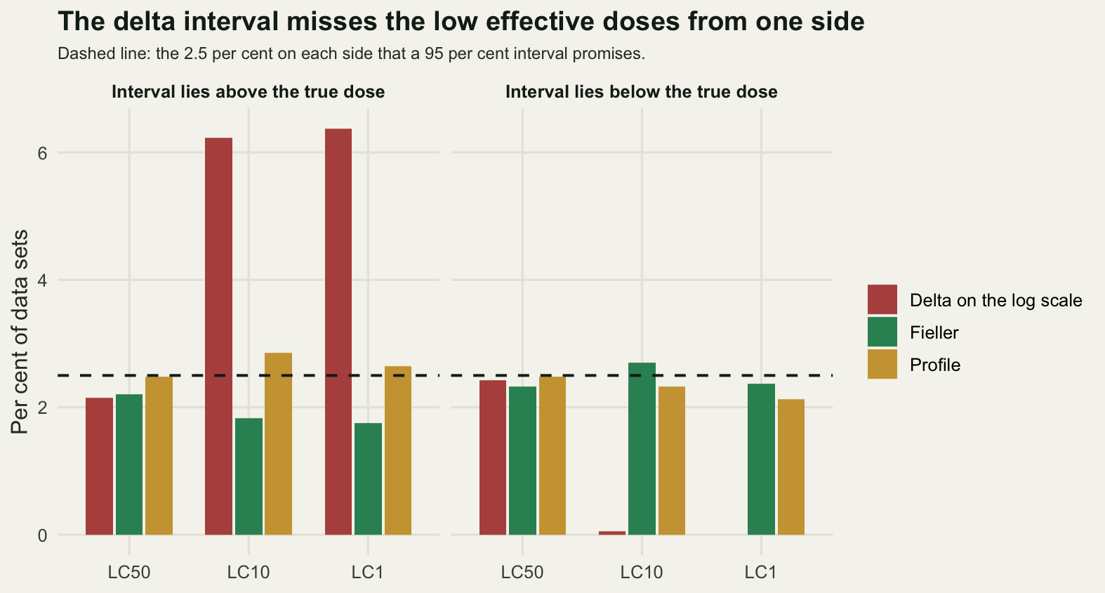

Figure 2: Where the 95 per cent intervals fail, split by side, over 4000 simulated data sets from the standard design. The left panel counts data sets whose whole interval lies above the true effective dose, the right panel those whose whole interval lies below it.

Two scales, two answers about which interval is wide

Everything above was measured on the \(\log_{10}\) concentration scale, where a width is a number of decades. Reports quote micrograms per litre. The two scales do not rank the three effective doses the same way, and the disagreement is not a subtlety.

wr <- cov_rows[, c("w_fieller", "w_fieller_dose")]
fold <- 10^cov_rows[, "w_fieller"]
print(round(cbind(log10_width = wr[, 1], fold_factor = fold,
                  dose_width = wr[, 2],
                  true_dose = lc_true(levs)), 4))

     log10_width fold_factor dose_width true_dose
LC50      0.3289      2.1325     9.2857   12.0000
LC10      0.7713      5.9066     2.2464    1.4577
LC1       1.5012     31.7135     0.4638    0.1461

round(c(log_width_lc10_over_lc50 = wr[2, 1] / wr[1, 1],
        log_width_lc1_over_lc50 = wr[3, 1] / wr[1, 1],
        dose_width_lc10_over_lc50 = wr[2, 2] / wr[1, 2],
        dose_width_lc1_over_lc50 = wr[3, 2] / wr[1, 2],
        fold_lc10_over_lc50 = as.numeric(fold[2] / fold[1]),
        fold_lc1_over_lc50 = as.numeric(fold[3] / fold[1])), 4)

 log_width_lc10_over_lc50   log_width_lc1_over_lc50 dose_width_lc10_over_lc50 
                   2.3452                    4.5645                    0.2419 
 dose_width_lc1_over_lc50       fold_lc10_over_lc50        fold_lc1_over_lc50 
                   0.0499                    2.7697                   14.8712 

On the log scale the median Fieller width is 0.3289 at the LC50, 0.7713 at the LC10 and 1.5012 at the LC1: the LC10 interval is 2.3452 times the LC50 interval and the LC1 interval 4.5645 times it. As a fold factor, which is how a toxicologist reads it, the LC50 is pinned to within a factor of 2.1325, the LC10 to 5.9066 and the LC1 to 31.7135.

Measured in micrograms per litre the ranking reverses. The median LC50 interval spans 9.2857 micrograms per litre, the LC10 interval 2.2464 and the LC1 interval 0.4638. The LC1 interval is 0.0499 of the width of the LC50 interval, twenty times narrower in the units the report uses. Anybody comparing absolute widths across effective doses will conclude that the LC1 is the best determined number in the table, when as a multiple it is the worst by a factor of 14.8712. The absolute width shrinks only because the doses themselves shrink. Uncertainty in an effective dose is multiplicative and has to be quoted that way.

Where the concentrations go

The animal count is fixed at 150 by cost and by the ethics committee. The concentrations are free. Four layouts, all with 150 animals, all analysed identically with Fieller intervals, over 3000 simulated tests each. Centred puts 4, 6, 9, 14, 21 and 32 micrograms per litre around the expected LC50, 25 animals at each, which is what a laboratory does when the LC50 is the deliverable. Wide is the standard 2 to 64 ladder from the start of the post. Low weighted uses 0.5, 1, 2, 4, 16 and 64 with 30, 30, 30, 25, 20 and 15 animals, putting four concentrations where the LC10 lives and keeping two up top to hold the slope. Very narrow uses 6, 8, 10, 14, 18 and 24, the layout of somebody who is confident about where the LC50 is.

set.seed(20260730)
designs <- list(
  Centred = list(conc = c(4, 6, 9, 14, 21, 32), n_an = rep(25, 6)),
  Wide = list(conc = c(2, 4, 8, 16, 32, 64), n_an = rep(25, 6)),
  "Low weighted" = list(conc = c(0.5, 1, 2, 4, 16, 64),
                        n_an = c(30, 30, 30, 25, 20, 15)),
  "Very narrow" = list(conc = c(6, 8, 10, 14, 18, 24), n_an = rep(25, 6)))
n_des <- 3000

for (nm in names(designs)) {
  xx <- log10(designs[[nm]]$conc)
  designs[[nm]]$x <- xx
  designs[[nm]]$p <- 1 / (1 + exp(-slope_true * (xx - x50_true)))
}
print(t(sapply(designs, function(dz) dz$conc)))

             [,1] [,2] [,3] [,4] [,5] [,6]
Centred       4.0    6    9   14   21   32
Wide          2.0    4    8   16   32   64
Low weighted  0.5    1    2    4   16   64
Very narrow   6.0    8   10   14   18   24

print(t(sapply(designs, function(dz) dz$n_an)))

             [,1] [,2] [,3] [,4] [,5] [,6]
Centred        25   25   25   25   25   25
Wide           25   25   25   25   25   25
Low weighted   30   30   30   25   20   15
Very narrow    25   25   25   25   25   25

print(round(t(sapply(designs, function(dz)
  c(total_animals = sum(dz$n_an), lowest_conc = min(dz$conc),
    highest_conc = max(dz$conc), lowest_response = min(dz$p),
    highest_response = max(dz$p)))), 4))

             total_animals lowest_conc highest_conc lowest_response
Centred                150         4.0           32          0.2414
Wide                   150         2.0           64          0.1338
Low weighted           150         0.5           64          0.0351
Very narrow            150         6.0           24          0.3268
             highest_response
Centred                0.7354
Wide                   0.8513
Low weighted           0.8513
Very narrow            0.6732

lev_sweep <- plogis(seq(qlogis(0.01), qlogis(0.6), length.out = 30))
sweep_rows <- NULL
sweep_curve <- NULL
for (nm in names(designs)) {
  dz <- designs[[nm]]
  Yd <- simulate_counts(dz$x, dz$n_an, n_des)
  fd <- fit_many(dz$x, dz$n_an, Yd)
  wid <- sapply(lev_sweep, function(lev) {
    bb <- fieller_log(lev, fd); median(bb[, 2] - bb[, 1]) })
  sweep_curve <- rbind(sweep_curve,
                       data.frame(design = nm, lev = lev_sweep, width = wid))
  row_out <- c(replicates = n_des)
  for (lev in levs) {
    bb <- fieller_log(lev, fd)
    wd <- bb[, 2] - bb[, 1]
    row_out <- c(row_out, median(wd), mean(!is.finite(wd)),
                 mean(bb[, 1] <= lx_true(lev) & bb[, 2] >= lx_true(lev)))
  }
  sweep_rows <- rbind(sweep_rows, row_out)
}
colnames(sweep_rows) <- c("replicates", paste0(rep(c("width", "unbounded",
                                                     "coverage"), 3),
                                               rep(c("_LC50", "_LC10", "_LC1"),
                                                   each = 3)))
rownames(sweep_rows) <- names(designs)
print(round(sweep_rows[, c(1, 2, 3, 4, 5, 6, 7)], 4))

             replicates width_LC50 unbounded_LC50 coverage_LC50 width_LC10
Centred            3000     0.3294         0.0073        0.9473     1.1499
Wide               3000     0.3289         0.0000        0.9520     0.7654
Low weighted       3000     0.4795         0.0000        0.9487     0.5748
Very narrow        3000     0.3902         0.1587        0.9550     2.2281
             unbounded_LC10 coverage_LC10
Centred              0.0073        0.9630
Wide                 0.0000        0.9560
Low weighted         0.0000        0.9527
Very narrow          0.1587        0.9737

print(round(sweep_rows[, c(8, 9, 10)], 4))

             width_LC1 unbounded_LC1 coverage_LC1
Centred         2.3642        0.0073       0.9627
Wide            1.4937        0.0000       0.9553
Low weighted    1.2000        0.0000       0.9527
Very narrow     4.6085        0.1587       0.9717

round(c(low_over_centred_lc10 = sweep_rows["Low weighted", "width_LC10"] /
          sweep_rows["Centred", "width_LC10"],
        low_over_centred_lc50 = sweep_rows["Low weighted", "width_LC50"] /
          sweep_rows["Centred", "width_LC50"],
        low_over_wide_lc10 = sweep_rows["Low weighted", "width_LC10"] /
          sweep_rows["Wide", "width_LC10"],
        centred_over_wide_lc50 = sweep_rows["Centred", "width_LC50"] /
          sweep_rows["Wide", "width_LC50"]), 4)

 low_over_centred_lc10  low_over_centred_lc50     low_over_wide_lc10 
                0.4999                 1.4558                 0.7509 
centred_over_wide_lc50 
                1.0016 

The low weighted layout halves the LC10 interval. Its median width is 0.5748 decades against the centred layout’s 1.1499, a ratio of 0.4999, and against the wide ladder’s 0.7654, a ratio of 0.7509. The price is the LC50: 0.4795 against 0.3294, a ratio of 1.4558. That is the trade any test programme should be stating out loud, roughly a factor of two won against a factor of one and a half lost.

The result I did not expect is the centred layout. Crowding the concentrations around the expected LC50 buys nothing at all for the LC50: a median width of 0.3294 against the wide ladder’s 0.3289, a ratio of 1.0016, which is a dead heat at this replicate count. It costs 1.1499 against 0.7654 at the LC10, half again as wide. The intuition that a layout aimed at the LC50 must be better at the LC50 is simply wrong, because what an LC50 estimate needs is not points near the LC50 but a well determined slope, and slope information comes from spread.

Push that further and the very narrow layout shows the failure mode. Its six concentrations produce true responses from 0.3268 to 0.6732, all inside the middle third of the curve, and it is worse than the wide ladder even at the LC50: 0.3902 against 0.3289. At the LC10 it is 2.2281, and in 0.1587 of data sets Fieller returns no bounded interval at all, because the slope cannot be told apart from zero. Its apparent LC10 coverage of 0.9737 is inflated by exactly those cases, since an interval with no upper end always contains the truth. That is what makes the design question harder than it looks: a layout can look precise and be reporting nothing.

Coverage stays close to nominal for the three usable layouts, between 0.9473 and 0.9630 across all three levels, so the width comparison above is between honest intervals rather than between an honest one and a broken one.

sweep_curve$design <- factor(sweep_curve$design, levels = names(designs))
des_cols <- c(Centred = te_pal$clay, Wide = te_pal$forest,
              "Low weighted" = te_pal$green, "Very narrow" = te_pal$gold)

ggplot(sweep_curve, aes(lev, width, colour = design)) +
  geom_line(linewidth = 1) +
  scale_x_continuous(trans = "logit", breaks = c(0.01, 0.05, 0.1, 0.2, 0.5),
                     labels = c("LC1", "LC5", "LC10", "LC20", "LC50")) +
  scale_y_continuous(trans = "log10", breaks = c(0.3, 0.5, 1, 2, 4),
                     labels = c("0.3", "0.5", "1.0", "2.0", "4.0")) +
  scale_colour_manual(values = des_cols, name = "Concentrations") +
  labs(x = "Effective dose being estimated",
       y = "Interval width (log10 concentration units)",
       title = "The concentration layout decides which effective dose is precise") +
  theme_te() +
  theme(legend.position = "right")

Figure 3: Median width of the Fieller interval, on the log10 concentration scale, for every effective dose between the LC1 and the LC50, under four concentration layouts that each use 150 animals.

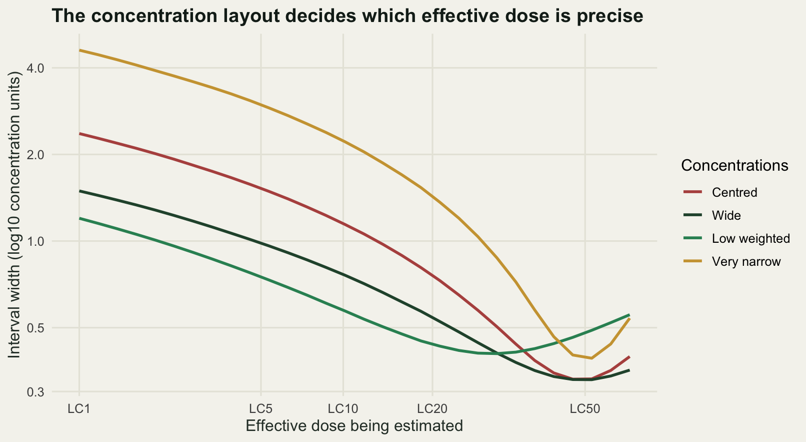
Animals cannot buy what the layout gives away

The obvious objection is that this is small beer next to sample size: put more animals in the centred layout and the interval will shrink. It will. The question is how many. The block below runs the centred layout at multiples of its animal count, up to twelve times, and asks where its LC10 interval finally matches what the low weighted layout achieved with 150 animals.

set.seed(20260730)
mult <- c(1, 2, 3, 4, 6, 8, 12)
target <- sweep_rows["Low weighted", "width_LC10"]
dz <- designs$Centred
grow <- t(sapply(mult, function(m) {
  Ym <- simulate_counts(dz$x, dz$n_an * m, 2000)
  fm <- fit_many(dz$x, dz$n_an * m, Ym)
  b10 <- fieller_log(0.1, fm); b50 <- fieller_log(0.5, fm)
  c(multiple = m, animals = sum(dz$n_an * m),
    width_LC10 = median(b10[, 2] - b10[, 1]),
    width_LC50 = median(b50[, 2] - b50[, 1]))
}))
print(round(grow, 4))

     multiple animals width_LC10 width_LC50
[1,]        1     150     1.1714     0.3332
[2,]        2     300     0.7090     0.2145
[3,]        3     450     0.5678     0.1730
[4,]        4     600     0.4817     0.1477
[5,]        6     900     0.3855     0.1190
[6,]        8    1200     0.3323     0.1028
[7,]       12    1800     0.2672     0.0832

n_need <- exp(approx(log(grow[, "width_LC10"]), log(grow[, "animals"]),
                     xout = log(target))$y)
sl_fit <- coef(lm(log(grow[, "width_LC10"]) ~ log(grow[, "animals"])))[2]
round(c(target_width = target, animals_needed = n_need,
        animals_needed_rounded = round(n_need),
        animal_factor = n_need / sum(dz$n_an),
        width_slope_against_animals = as.numeric(sl_fit)), 4)

               target_width              animals_needed 
                     0.5748                    440.1057 
     animals_needed_rounded               animal_factor 
                   440.0000                      2.9340 
width_slope_against_animals 
                    -0.5854 

Width falls with animal count at a fitted log-log slope of -0.5854, close enough to a square root law that interpolating between the simulated points is safe. On that curve the centred layout reaches the target width of 0.5748 at 440 animals, a factor of 2.9340 on the 150 it started with. Three times the animals to buy back what moving six concentrations down the scale gives away for nothing.

Two smaller things are worth reading off the same table. The first row of this run gives an LC10 width of 1.1714 for the centred layout, against 1.1499 from the design sweep in the previous section; the two are independent estimates of the same quantity, and the gap between them is the Monte Carlo noise on a median width at these replicate counts. And the LC50 column shows the extra animals are not wasted in general: at 450 animals the centred layout’s LC50 interval is down to 0.1730 from 0.3332. Animals do buy precision. They are an expensive way to buy the particular precision that the layout was throwing away.

gd <- data.frame(animals = grow[, "animals"], width = grow[, "width_LC10"])

ggplot(gd, aes(animals, width)) +
  geom_hline(yintercept = target, colour = te_pal$green, linewidth = 1) +
  geom_segment(x = log10(n_need), xend = log10(n_need), y = 0.2, yend = target,
               colour = te_pal$ink, linetype = "dashed", linewidth = 0.6) +
  geom_line(colour = te_pal$clay, linewidth = 1) +
  geom_point(colour = te_pal$clay, size = 2.6) +
  geom_point(aes(x = n_need, y = target), colour = te_pal$ink, shape = 4,
             size = 4, stroke = 1.3) +
  annotate("text", x = 470, y = 0.95,
           label = "440 animals in the centred layout", hjust = 0, size = 3.2,
           colour = "#2c3a31") +
  annotate("text", x = 700, y = target + 0.06,
           label = "low weighted layout, 150 animals", hjust = 0, size = 3.2,
           colour = "#2c3a31") +
  scale_x_continuous(trans = "log10", breaks = c(150, 300, 600, 1200, 1800),
                     labels = c("150", "300", "600", "1200", "1800")) +
  labs(x = "Animals in the test (log scale)",
       y = "LC10 interval width (log10 concentration units)",
       title = "Nearly three times the animals buys what the layout gives away") +
  theme_te()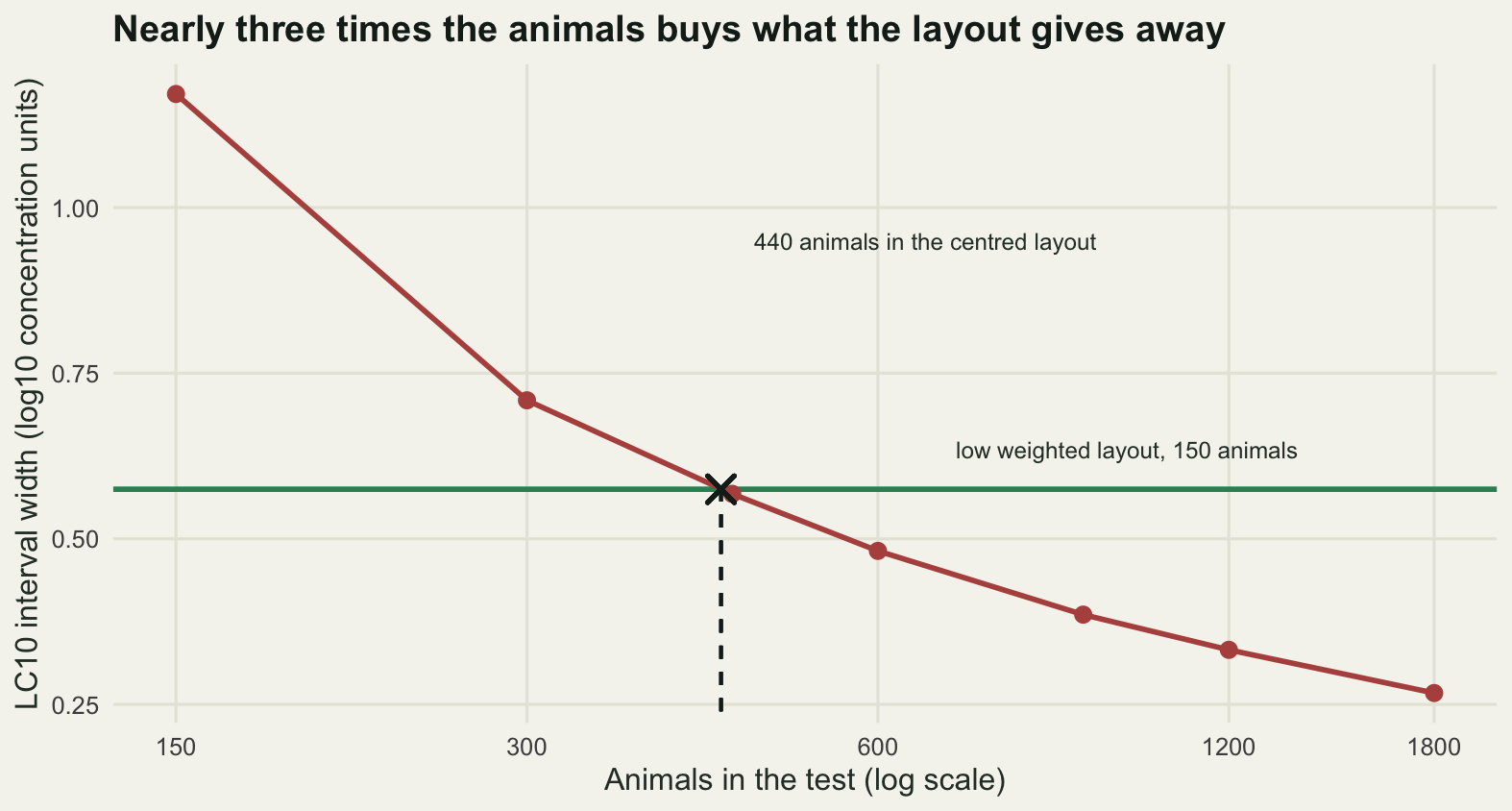

Warning in geom_point(aes(x = n_need, y = target), colour = te_pal$ink, : All aesthetics have length 1, but the data has 7 rows.
ℹ Please consider using `annotate()` or provide this layer with data containing
  a single row.

Figure 4: Median LC10 interval width for the centred layout as its animal count grows, against the width the low weighted layout reaches with 150 animals (the horizontal line). The cross marks where the two meet.

The honest limit

Every layout above was chosen knowing the answer. The concentrations were placed by somebody who had been told the LC50 is 12 and the slope is 2.4, which is the one thing a first test cannot know. So the last measurement asks what happens when that guess is wrong by a factor of three in either direction, with the layouts left exactly as they are.

set.seed(20260730)
truths <- c(4, 12, 36)
mis <- NULL
for (tl in truths) {
  for (nm in c("Centred", "Wide", "Low weighted")) {
    dz <- designs[[nm]]
    Ym <- simulate_counts(dz$x, dz$n_an, 2000, x50 = log10(tl))
    fm <- fit_many(dz$x, dz$n_an, Ym)
    b10 <- fieller_log(0.1, fm); b50 <- fieller_log(0.5, fm)
    mis <- rbind(mis, c(true_lc50 = tl, design = which(names(designs) == nm),
                        width_LC50 = median(b50[, 2] - b50[, 1]),
                        width_LC10 = median(b10[, 2] - b10[, 1]),
                        unbounded = mean(!is.finite(b10[, 2] - b10[, 1]))))
  }
}
mis <- data.frame(design = names(designs)[mis[, "design"]],
                  true_lc50 = mis[, "true_lc50"],
                  width_LC50 = round(mis[, "width_LC50"], 4),
                  width_LC10 = round(mis[, "width_LC10"], 4),
                  unbounded = round(mis[, "unbounded"], 4))
print(mis)

        design true_lc50 width_LC50 width_LC10 unbounded
1      Centred         4     0.6456     1.9675    0.0290
2         Wide         4     0.4092     1.0627    0.0000
3 Low weighted         4     0.3773     0.6436    0.0000
4      Centred        12     0.3256     1.1259    0.0065
5         Wide        12     0.3289     0.7651    0.0000
6 Low weighted        12     0.4796     0.5731    0.0000
7      Centred        36     0.7281     0.8755    0.0380
8         Wide        36     0.4280     0.6781    0.0000
9 Low weighted        36     0.6595     0.6270    0.0000

round(c(low_over_centred_lc10_at_true_4 =
          mis$width_LC10[mis$true_lc50 == 4 & mis$design == "Low weighted"] /
          mis$width_LC10[mis$true_lc50 == 4 & mis$design == "Centred"],
        low_lc10_spread_across_truths = max(mis$width_LC10[mis$design == "Low weighted"]) /
          min(mis$width_LC10[mis$design == "Low weighted"]),
        centred_lc50_spread_across_truths = max(mis$width_LC50[mis$design == "Centred"]) /
          min(mis$width_LC50[mis$design == "Centred"])), 4)

  low_over_centred_lc10_at_true_4     low_lc10_spread_across_truths 
                           0.3271                            1.1230 
centred_lc50_spread_across_truths 
                           2.2362 

The circularity turns out to bite the centred layout hardest, not the low weighted one. Move the true LC50 down to 4 and the centred layout’s LC50 interval goes from 0.3256 to 0.6456 decades and its LC10 interval to 1.9675, with 0.0290 of data sets giving no bounded interval. Move it up to 36 and the LC50 width is 0.7281 with 0.0380 unbounded. Across the three truths the centred layout’s LC50 width varies by a factor of 2.2362. The low weighted layout’s LC10 width varies by a factor of 1.1230, from 0.5731 to 0.6436, and it is the best of the three at the LC10 under all three truths, including the case where the substance turns out three times more toxic than assumed, where it beats the centred layout by a ratio of 0.3271. A layout that spreads its concentrations to catch a low response level also catches a mislocated curve, and the prior guess it needs is much weaker than the guess the centred layout needs.

Three limits the study does not cover. All of it conditions on the log-logistic form being right, and the intervals here are conditional intervals: they carry no allowance for the choice of link function, which the companion post measured and found to matter most at exactly these low response levels, so the real uncertainty in an LC10 is wider than any interval above. The counts are independent binomial draws with no vessel to vessel correlation, which is the assumption that most often fails in a real acute test and which checking a dose-response analysis takes apart. And the low weighted layout was picked by hand from a few candidates rather than optimised, so a formal design calculation for the LC10 would do better than 0.5748, which makes the gain measured here a lower bound on what design work can buy.

Where to go next

If the interval is worth computing, it is worth knowing what else moves it. The link function is the first thing, and dose-response curves and the LC50 measures how far apart probit, logit and complementary log-log drift as the response level falls, a source of spread that sits on top of everything measured here. If the response is not monotone then none of these intervals mean what they say, and hormesis and non-monotonic responses shows what a stimulatory low dose region does to a fitted effective dose.

On the design side the natural next step is to stop choosing layouts by hand. The width surface computed in the sweep above is a crude design criterion already, and the same simulate and measure loop will optimise over concentration placement given a prior guess at the curve, which is the approach power analysis by simulation takes for the two group case.

References

Fieller EC 1954 Journal of the Royal Statistical Society Series B 16(2):175-185 (10.1111/j.2517-6161.1954.tb00159.x)

Ritz C 2010 Environmental Toxicology and Chemistry 29(1):220-229 (10.1002/etc.7)

Ritz C, Baty F, Streibig JC, Gerhard D 2015 PLOS ONE 10(12):e0146021 (10.1371/journal.pone.0146021)

Venables WN, Ripley BD 2002 Modern Applied Statistics with S, fourth edition. Springer, ISBN 978-0-387-95457-8

Related tutorials

• Dose-response curves and the LC50
• Return levels and uncertainty
• Power analysis by simulation
• Checking a dose-response analysis