library(ggplot2)

te_pal <- list(forest = "#275139", green = "#2f8f63", sage = "#93a87f",
               clay = "#b5534e", gold = "#cda23f", line = "#dad9ca",
               ink = "#16241d", paper = "#f5f4ee")

theme_te <- function() {
  theme_minimal(base_size = 12) +
    theme(panel.grid.minor = element_blank(),
          panel.grid.major = element_line(colour = "#e7e6dc"),
          plot.background = element_rect(fill = "#f5f4ee", colour = NA),
          panel.background = element_rect(fill = "#f5f4ee", colour = NA),
          plot.title = element_text(face = "bold", colour = te_pal$ink),
          axis.title = element_text(colour = "#2c3a31"))
}Dose-response curves and the LC50
R
ecotoxicology
GLM
ecology tutorial
ggplot2
Fit a dose-response curve in R with three binomial links: the LC50 barely moves, the LC10 moves, and AIC spots the asymmetric link but not probit against logit.
A laboratory runs a 48 hour acute test on Daphnia magna. Seven concentrations in a doubling series, twenty-five animals at each, and at the end somebody counts how many animals are immobilised. The count sheet has seven rows on it. What leaves the building is a single number, the LC50, and increasingly a second one: a low-effect concentration such as the LC10, which is what a risk assessment divides by an assessment factor to get a threshold. Neither number is on the count sheet. Both are read off a curve that was fitted to it, at a place on that curve chosen by a regulation.
That is the whole subject of this tutorial. An effective dose is a quantile of a fitted curve, so it inherits everything the curve family assumes, and it inherits more of it the further from the middle of the data you read. This post fits the same seven counts with a probit, a logit and a complementary log-log link and measures how far the answer moves. The short version of the measurements below: at the LC50 the two symmetric links agree to within a ratio of 1.0022 and the asymmetric one does not agree at all; at the LC1 the three answers span more than a factor of two; and over 300 simulated experiments from each of three generating links AIC recovers the right link in 0.5778 of them, and on data generated by a logit it prefers the probit more often than the logit.
The fitting machinery is the binomial GLM of Logistic regression for presence-absence data, and nothing here changes it. What changes is the question put to the fit. There, the object of interest is a coefficient, an estimate of how strongly a predictor moves the probability. Here the coefficients are a nuisance and the object of interest is a ratio of them, the concentration at which the curve crosses a stated level. Ratios of estimates are worse behaved than the estimates they are built from, which is why this post keeps returning to the same measurement. The log-logistic distribution also appears in Parametric survival and the AFT model, where it runs along a time axis and the quantity read off it is a survival time; here the same algebra runs along a concentration axis at a fixed observation time, and the quantity read off it is a dose. The R package written for this work is drc. Everything below uses glm instead, so that each step is visible.
A doubling series, and three curves that agree at the LC50
The design is the standard one: concentrations of 0.8, 1.6, 3.2, 6.4, 12.8, 25.6 and 51.2 micrograms per litre, twenty-five animals at each, 175 animals in total, scored at 48 hours. A range-finding test has already put the LC50 somewhere near 10, which is why the series is centred where it is.
The generating curve needs a link, and any choice of link is a choice about the shape of the tails, so all three are set up here on equal terms. Each truth is a straight line on log concentration through its own link, each passes through a response of one half at exactly 9 micrograms per litre, and each has the same steepness there: a slope of 0.65 in response per natural log unit of concentration, at the point where the response is one half. The three generating curves are therefore indistinguishable at the LC50 and as close as three different functional forms can be made in the middle of the design.
conc  <- c(0.8, 1.6, 3.2, 6.4, 12.8, 25.6, 51.2)
n_per <- 25
lc50_true  <- 9
slope_mid  <- 0.65
links <- c("logit", "probit", "cloglog")
lev   <- c(0.5, 0.2, 0.1, 0.05, 0.01)

link_q <- function(p, link) switch(link, logit = log(p / (1 - p)),
                                   probit = qnorm(p), cloglog = log(-log(1 - p)))
link_p <- function(eta, link) switch(link, logit = plogis(eta),
                                     probit = pnorm(eta), cloglog = 1 - exp(-exp(eta)))
dens_half <- function(link) switch(link, logit = 0.25, probit = dnorm(0),
                                   cloglog = log(2) / 2)
slope_of <- function(link) slope_mid / dens_half(link)
true_p  <- function(x, link)
  link_p(link_q(0.5, link) + slope_of(link) * (log(x) - log(lc50_true)), link)
true_lc <- function(p, link)
  exp(log(lc50_true) + (link_q(p, link) - link_q(0.5, link)) / slope_of(link))

c(concentrations = length(conc), animals_each = n_per,
  animals_total = length(conc) * n_per, test_duration_hours = 48,
  true_lc50 = lc50_true, slope_at_lc50 = slope_mid)
concentrations animals_each animals_total test_duration_hours
7.00 25.00 175.00 48.00
true_lc50 slope_at_lc50
9.00 0.65 print(c(response_levels_percent = 100 * lev))response_levels_percent1 response_levels_percent2 response_levels_percent3
50 20 10
response_levels_percent4 response_levels_percent5
5 1 print(round(rbind(concentration = conc, true_response = true_p(conc, "logit")), 4)) [,1] [,2] [,3] [,4] [,5] [,6] [,7]
concentration 0.8000 1.6000 3.2000 6.4000 12.8000 25.6000 51.2000
true_response 0.0018 0.0111 0.0636 0.2919 0.7142 0.9381 0.9892print(round(sapply(links, slope_of), 4)) logit probit cloglog
2.6000 1.6293 1.8755 truth_tab <- sapply(links, function(l) sapply(lev, function(p) true_lc(p, l)))
rownames(truth_tab) <- paste0("LC", 100 * lev)
print(round(cbind(truth_tab,
spread = apply(truth_tab, 1, function(z) max(z) / min(z))), 4)) logit probit cloglog spread
LC50 9.0000 9.0000 9.0000 1.0000
LC20 5.2806 5.3692 4.9180 1.0917
LC10 3.8657 4.0987 3.2962 1.2435
LC5 2.9001 3.2795 2.2456 1.4604
LC1 1.5371 2.1585 0.9417 2.2922Under the logit truth the seven concentrations produce expected responses of 0.0018, 0.0111, 0.0636, 0.2919, 0.7142, 0.9381 and 0.9892. That is a well-shaped experiment by any standard: the LC50 sits between the fourth and fifth concentration, and there is a real gradient across the whole series rather than a jump from nothing to everything.
The last table is worth a pause, because it is written before any data exist. Three curves that are identical at the LC50 and equally steep there have LC10 values of 3.8657, 4.0987 and 3.2962. By the LC1 they read 1.5371, 2.1585 and 0.9417, a spread of 2.2922 between the largest and the smallest. No estimation has happened yet. The disagreement is a property of the three functional forms, sitting there before the first animal is counted, and estimation can only add to it.
Recovering an LC50 that we already know
One dataset, drawn from the logit truth. The counts are what a technician would write down.
set.seed(20260729)
dead <- rbinom(length(conc), n_per, true_p(conc, "logit"))
print(rbind(concentration = conc, immobilised = dead,
            proportion = round(dead / n_per, 4)))
[,1] [,2] [,3] [,4] [,5] [,6] [,7]
concentration 0.8 1.60 3.2 6.40 12.80 25.60 51.2
immobilised 0.0 1.00 0.0 8.00 19.00 23.00 25.0
proportion 0.0 0.04 0.0 0.32 0.76 0.92 1.0c(immobilised_total = sum(dead), animals_total = length(conc) * n_per)immobilised_total animals_total
76 175 In total 76 of the 175 animals were immobilised. Note the shape of the low end: none at 0.8, one at 1.6, none at 3.2. That non-monotone run is ordinary sampling noise, and it is also the entire empirical content of the region where a low-effect concentration will later be read off.
Fitting is one line. The estimate of a level-p effective dose is the concentration at which the linear predictor equals the link function evaluated at p, which is a ratio of two estimated coefficients. Two intervals are worth having. The delta method gives a standard error on the log concentration scale by linearising that ratio. Fieller’s theorem does better: it inverts the test that the linear predictor equals its target value at a given concentration, which handles the ratio exactly rather than by first-order approximation, and it can return an unbounded interval when the slope is poorly determined, which is honest rather than a defect.
n_warn <- 0
fit_link <- function(y, link)
  withCallingHandlers(
    glm(cbind(y, n_per - y) ~ log(conc), family = binomial(link = link)),
    warning = function(w) { n_warn <<- n_warn + 1; invokeRestart("muffleWarning") })

lc_hat <- function(fit, p, link) {
  b <- coef(fit)
  unname(exp((link_q(p, link) - b[1]) / b[2]))
}
lc_se_log <- function(fit, p, link) {
  b <- coef(fit); V <- vcov(fit); q <- link_q(p, link)
  g <- c(-1 / b[2], -(q - b[1]) / b[2]^2)
  sqrt(as.numeric(t(g) %*% V %*% g))
}
fieller <- function(fit, p, link, conf = 0.95) {
  b <- coef(fit); V <- vcov(fit); q <- link_q(p, link)
  z <- qnorm(1 - (1 - conf) / 2)
  aa <- b[2]^2 - z^2 * V[2, 2]
  bb <- 2 * (b[2] * (b[1] - q) - z^2 * V[1, 2])
  cc <- (b[1] - q)^2 - z^2 * V[1, 1]
  disc <- bb^2 - 4 * aa * cc
  if (aa <= 0 || disc < 0) return(c(NA_real_, NA_real_))
  unname(exp(sort(c((-bb - sqrt(disc)) / (2 * aa), (-bb + sqrt(disc)) / (2 * aa)))))
}

f_logit <- fit_link(dead, "logit")
print(round(summary(f_logit)$coefficients, 4))
Estimate Std. Error z value Pr(>|z|)
(Intercept) -5.9063 0.9554 -6.1822 0
log(conc) 2.7143 0.4217 6.4374 0round(c(residual_deviance = deviance(f_logit),
residual_df = df.residual(f_logit),
lack_of_fit_p = pchisq(deviance(f_logit), df.residual(f_logit),
lower.tail = FALSE),
warnings_so_far = n_warn), 4)residual_deviance residual_df lack_of_fit_p warnings_so_far
5.4364 5.0000 0.3650 0.0000 one_row <- function(p) {
ci <- fieller(f_logit, p, "logit")
c(estimate = lc_hat(f_logit, p, "logit"), se_log = lc_se_log(f_logit, p, "logit"),
fieller_lower = ci[1], fieller_upper = ci[2], truth = true_lc(p, "logit"))
}
print(round(rbind(LC50 = one_row(0.5), LC10 = one_row(0.1)), 4)) estimate se_log fieller_lower fieller_upper truth
LC50 8.8108 0.1013 7.1575 10.8594 9.0000
LC10 3.9216 0.1607 2.5692 5.0794 3.8657The fitted slope is 2.7143 against a true 2.6, the residual deviance is 5.4364 on 5 degrees of freedom, and the lack-of-fit probability is 0.3650. The LC50 comes out at 8.8108 against a truth of 9, with a standard error of 0.1013 on the log scale and a Fieller interval running from 7.1575 to 10.8594. The LC10 comes out at 3.9216 against a truth of 3.8657, with an interval from 2.5692 to 5.0794. Both are correct, and the second interval is already noticeably wider relative to its centre than the first.
One dataset proves nothing about an estimator, so the same experiment is run 2000 times.
set.seed(20260729)
n_sim <- 2000
cal <- t(sapply(seq_len(n_sim), function(i) {
  y <- rbinom(length(conc), n_per, true_p(conc, "logit"))
  f <- fit_link(y, "logit")
  ci <- lapply(c(0.5, 0.1, 0.01), function(p) fieller(f, p, "logit"))
  hit <- function(k, p) ci[[k]][1] < true_lc(p, "logit") &&
    true_lc(p, "logit") < ci[[k]][2]
  c(lc50 = lc_hat(f, 0.5, "logit"), lc10 = lc_hat(f, 0.1, "logit"),
    cov50 = hit(1, 0.5), cov10 = hit(2, 0.1), cov1 = hit(3, 0.01),
    wid50 = ci[[1]][2] / ci[[1]][1], wid10 = ci[[2]][2] / ci[[2]][1],
    wid1 = ci[[3]][2] / ci[[3]][1])
}))
c(datasets = n_sim, unbounded_intervals = sum(is.na(cal[, "cov50"])),
  warnings_so_far = n_warn)
datasets unbounded_intervals warnings_so_far
2000 0 0 round(c(median_lc50 = median(cal[, "lc50"]), true_lc50 = lc50_true,
median_lc10 = median(cal[, "lc10"]), true_lc10 = true_lc(0.1, "logit"),
coverage_lc50 = mean(cal[, "cov50"]), coverage_lc10 = mean(cal[, "cov10"]),
coverage_lc1 = mean(cal[, "cov1"]),
median_width_ratio_lc50 = median(cal[, "wid50"]),
median_width_ratio_lc10 = median(cal[, "wid10"]),
median_width_ratio_lc1 = median(cal[, "wid1"])), 4) median_lc50 true_lc50 median_lc10
9.0546 9.0000 3.9083
true_lc10 coverage_lc50 coverage_lc10
3.8657 0.9575 0.9560
coverage_lc1 median_width_ratio_lc50 median_width_ratio_lc10
0.9540 1.5229 1.9901
median_width_ratio_lc1
3.3890 The machinery is calibrated. The median estimate over 2000 experiments is 9.0546 for an LC50 of 9 and 3.9083 for an LC10 of 3.8657. The Fieller intervals cover at 0.9575, 0.9560 and 0.9540 for the LC50, the LC10 and the LC1, which is what a nominal 0.95 procedure should do, and not one of the 2000 returned an unbounded interval on this design.
The interval widths are the interesting column. Expressed as the ratio of the upper limit to the lower, the median LC50 interval spans a factor of 1.5229, the LC10 interval 1.9901, and the LC1 interval 3.3890. Same animals, same fit, same nominal confidence: the further down the curve the question is asked, the wider the answer, and that is with the model form known to be exactly right. It is not right in any real analysis, which is the rest of this post.
The same seven counts through three links
Now fit all three links to the identical counts and read the same five levels off each.
fits <- lapply(links, function(l) fit_link(dead, l))
names(fits) <- links
lc_tab <- sapply(links, function(l) sapply(lev, function(p) lc_hat(fits[[l]], p, l)))
rownames(lc_tab) <- paste0("LC", 100 * lev)
print(round(lc_tab, 4))
logit probit cloglog
LC50 8.8108 8.7779 10.1582
LC20 5.2870 4.9292 5.1949
LC10 3.9216 3.6456 3.3323
LC5 2.9779 2.8418 2.1766
LC1 1.6210 1.7810 0.8298print(round(cbind(lc_tab,
spread = apply(lc_tab, 1, function(z) max(z) / min(z)),
logit_vs_probit = lc_tab[, "logit"] / lc_tab[, "probit"],
truth = sapply(lev, function(p) true_lc(p, "logit"))), 4)) logit probit cloglog spread logit_vs_probit truth
LC50 8.8108 8.7779 10.1582 1.1573 1.0038 9.0000
LC20 5.2870 4.9292 5.1949 1.0726 1.0726 5.2806
LC10 3.9216 3.6456 3.3323 1.1768 1.0757 3.8657
LC5 2.9779 2.8418 2.1766 1.3681 1.0479 2.9001
LC1 1.6210 1.7810 0.8298 2.1464 0.9102 1.5371aics <- sapply(fits, AIC)
print(round(rbind(deviance = sapply(fits, deviance), aic = aics,
delta_aic = aics - min(aics)), 4)) logit probit cloglog
deviance 5.4364 6.4102 8.3931
aic 20.8675 21.8413 23.8241
delta_aic 0.0000 0.9738 2.9567At the LC50 the logit gives 8.8108 and the probit 8.7779, a ratio of 1.0038. Anyone who has been told that probit and logit hardly matter for an LC50 has been told the truth: on this dataset that difference sits inside the Fieller interval, and over the 2000 simulated experiments the median interval spans a factor of 1.5229. It is invisible.
The complementary log-log link gives 10.1582, a disagreement of a different size: the three-way spread at the LC50 is 1.1573 against the 1.0038 above, and the whole of it comes from the asymmetric link. That estimate is still inside the Fieller interval, so one draw cannot settle it, and the next section puts the question to an infinitely large experiment instead. The answer there is the first thing the measurement adds to the folklore: agreement at the LC50 is a property of symmetric links, not a property of link functions.
Down the curve the picture changes for everyone. At the LC10 the three estimates are 3.9216, 3.6456 and 3.3323, a spread of 1.1768, and the symmetric pair are separated by 1.0757. At the LC1 they read 1.6210, 1.7810 and 0.8298: a spread of 2.1464, with the complementary log-log answer well below the probit one. If a threshold were set by dividing an LC1 by an assessment factor, the choice of link would be worth more than a factor of 1.5 in the final number.
The residual deviances are 5.4364, 6.4102 and 8.3931, and the AIC differences are 0, 0.9738 and 2.9567. The correct link is at the top on this run, which is reassuring for about a second: nothing in that column would let a reviewer reject the complementary log-log fit, and the two symmetric fits sit within about one AIC unit of each other.
grid_hi <- exp(seq(log(0.55), log(72), length.out = 400))
curve_df <- do.call(rbind, lapply(links, function(l)
  data.frame(x = grid_hi,
             p = link_p(coef(fits[[l]])[1] + coef(fits[[l]])[2] * log(grid_hi), l),
             link = l)))
curve_df$link <- factor(curve_df$link, levels = links)
obs_df <- data.frame(x = conc, p = dead / n_per)
link_cols <- c(logit = te_pal$forest, probit = te_pal$gold, cloglog = te_pal$clay)

ggplot(curve_df, aes(x, p, colour = link)) +
  geom_line(linewidth = 0.9) +
  geom_point(data = obs_df, aes(x, p), inherit.aes = FALSE, size = 2.6,
             colour = te_pal$ink) +
  scale_x_log10(breaks = conc, labels = conc) +
  scale_colour_manual(values = link_cols, name = NULL) +
  labs(x = "Concentration (ug per litre)", y = "Proportion immobilised",
       title = "All three links describe the tested concentrations equally well") +
  theme_te() +
  theme(legend.position = "top")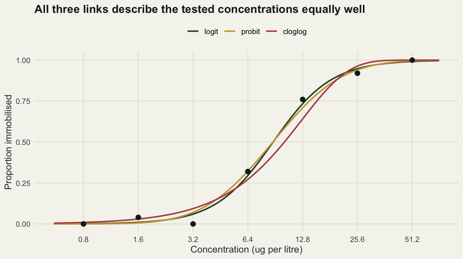
Where the three curves part company
The dataset above carries sampling noise, so it cannot separate what the links do from what the draw did. The clean way to ask is to hand each link an infinite dataset from the same generating curve. That is what a misspecified maximum likelihood estimator converges to: the parameter values that minimise the Kullback-Leibler divergence from the truth, which for grouped binomial data is the expected deviance. Minimising it directly with optim gives the large-sample fit of each link with no noise in it at all.
kl_fit <- function(true_link, link) {
  pt <- true_p(conc, true_link)
  start <- c(link_q(0.5, link) - slope_of(link) * log(lc50_true), slope_of(link))
  obj <- function(b) {
    ph <- link_p(b[1] + b[2] * log(conc), link)
    ph <- pmin(pmax(ph, 1e-12), 1 - 1e-12)
    -sum(n_per * (pt * log(ph) + (1 - pt) * log(1 - ph)))
  }
  optim(start, obj, method = "BFGS", control = list(reltol = 1e-12))$par
}
asym_b <- lapply(links, function(l) kl_fit("logit", l))
names(asym_b) <- links
asym_tab <- sapply(links, function(l)
  sapply(lev, function(p) exp((link_q(p, l) - asym_b[[l]][1]) / asym_b[[l]][2])))
rownames(asym_tab) <- paste0("LC", 100 * lev)
print(round(cbind(asym_tab,
                  spread = apply(asym_tab, 1, function(z) max(z) / min(z)),
                  logit_vs_probit = asym_tab[, "logit"] / asym_tab[, "probit"],
                  truth = sapply(lev, function(p) true_lc(p, "logit"))), 4))
logit probit cloglog spread logit_vs_probit truth
LC50 9.0000 8.9805 10.4376 1.1623 1.0022 9.0000
LC20 5.2806 4.9716 5.0593 1.0621 1.0621 5.2806
LC10 3.8657 3.6497 3.1323 1.2342 1.0592 3.8657
LC5 2.9001 2.8275 1.9775 1.4666 1.0257 2.9001
LC1 1.5371 1.7517 0.6979 2.5098 0.8775 1.5371print(round(rbind(true_response = true_p(conc, "logit"),
sapply(conc, function(x)
sapply(links, function(l)
link_p(asym_b[[l]][1] + asym_b[[l]][2] * log(x), l)))), 4)) [,1] [,2] [,3] [,4] [,5] [,6] [,7]
true_response 0.0018 0.0111 0.0636 0.2919 0.7142 0.9381 0.9892
logit 0.0018 0.0111 0.0636 0.2919 0.7142 0.9381 0.9892
probit 0.0003 0.0070 0.0710 0.3148 0.6930 0.9320 0.9934
cloglog 0.0124 0.0362 0.1032 0.2756 0.6148 0.9405 0.9998With the noise removed, the logit recovers its own truth exactly, as it must. The probit lands on 8.9805 at the LC50, 3.6497 at the LC10 and 1.7517 at the LC1, so it tracks the logit closely in the middle and drifts away from it downwards. The complementary log-log fit lands on 10.4376, 3.1323 and 0.6979, and its LC1 is less than half the logit value. The three-way spread is 1.1623 at the LC50, dips to 1.0621 at the LC20 where the complementary log-log curve crosses the other two, then climbs to 1.2342 at the LC10, 1.4666 at the LC5 and 2.5098 at the LC1.
The second table says where that comes from. At 0.8 micrograms per litre the true response is 0.0018, the large-sample complementary log-log fit predicts 0.0124 and the probit predicts 0.0003. At 3.2 the truth is 0.0636 and the complementary log-log fit says 0.1032. None of that could be caught by eye on a plot of the fitted curves, because 0.0124 and 0.0018 are both a flat line along the bottom of the panel. It is exactly the error that matters when the reported quantity is the concentration at which the response reaches one tenth.
Now count the evidence available in that region.
lc10_logit <- lc_hat(fits[["logit"]], 0.1, "logit")
below <- conc < lc10_logit
c(concentrations_below_estimated_lc10 = sum(below),
  animals_below = sum(below) * n_per, immobilised_below = sum(dead[below]),
  lowest_tested = min(conc))
concentrations_below_estimated_lc10 animals_below
3.0 75.0
immobilised_below lowest_tested
1.0 0.8 grid_lo <- exp(seq(log(0.05), log(60), length.out = 2000))
pred_m <- sapply(links, function(l)
link_p(coef(fits[[l]])[1] + coef(fits[[l]])[2] * log(grid_lo), l))
ratio_lo <- apply(pred_m, 1, function(z) max(z) / min(z))
sep_dose <- function(thr) max(grid_lo[ratio_lo > thr])
round(c(spread_exceeds_1.5_below = sep_dose(1.5),
spread_exceeds_2_below = sep_dose(2),
spread_exceeds_5_below = sep_dose(5),
logit_response_at_that_dose = unname(link_p(coef(fits[["logit"]])[1] +
coef(fits[["logit"]])[2] * log(sep_dose(2)), "logit"))), 4) spread_exceeds_1.5_below spread_exceeds_2_below
3.3324 2.4738
spread_exceeds_5_below logit_response_at_that_dose
1.5435 0.0308 Three of the seven concentrations sit below the estimated LC10, so 75 animals were tested there. One of them was immobilised. That single animal is the entire observational basis for the part of the curve a low-effect concentration is read from; everything else the fit knows about that region it knows by assuming a shape and continuing it downwards from where the responses were common.
The predicted responses of the three fits differ by more than a factor of 1.5 below 3.3324 micrograms per litre, by more than a factor of 2 below 2.4738, and by more than a factor of 5 below 1.5435. The lowest concentration actually tested is 0.8, so the separation does not begin outside the design at all: it begins inside it, at a concentration where the logit fit predicts a response of 0.0308, which no group of twenty-five animals can tell apart from a different curve shape.
tail_df <- do.call(rbind, lapply(links, function(l)
  data.frame(x = grid_lo, p = link_p(coef(fits[[l]])[1] +
                                       coef(fits[[l]])[2] * log(grid_lo), l), link = l)))
tail_df <- tail_df[tail_df$x >= 0.35 & tail_df$x <= 14, ]
tail_df$link <- factor(tail_df$link, levels = links)
lc10_df <- data.frame(x = sapply(links, function(l) lc_hat(fits[[l]], 0.1, l)),
                      link = factor(links, levels = links))
floor_p <- 5e-4
seen <- obs_df[obs_df$x <= 14, ]
zero_df <- seen[seen$p == 0, ]
zero_df$p <- floor_p

ggplot(tail_df, aes(x, p, colour = link)) +
  geom_hline(yintercept = 0.1, linetype = "dashed", colour = "#5d6b61") +
  geom_line(linewidth = 0.9) +
  geom_segment(data = lc10_df, aes(x = x, xend = x, y = 0.05, yend = 0.2),
               linewidth = 1.1) +
  geom_point(data = seen[seen$p > 0, ], aes(x, p), inherit.aes = FALSE,
             size = 2.6, colour = te_pal$ink) +
  geom_point(data = zero_df, aes(x, p), inherit.aes = FALSE, size = 2.6,
             shape = 6, colour = te_pal$ink) +
  scale_x_log10(breaks = c(0.4, 0.8, 1.6, 3.2, 6.4, 12.8)) +
  scale_y_log10(breaks = c(0.001, 0.003, 0.01, 0.03, 0.1, 0.3),
                labels = c("0.001", "0.003", "0.01", "0.03", "0.1", "0.3")) +
  scale_colour_manual(values = link_cols, name = NULL) +
  coord_cartesian(ylim = c(4e-4, 0.45)) +
  labs(x = "Concentration (ug per litre)", y = "Proportion immobilised",
       title = "Below a ten per cent response the three fits stop agreeing",
       subtitle = paste("Open triangles: doses at which no animal was immobilised",
                        "(zero has no place on a log axis)")) +
  theme_te() +
  theme(legend.position = "top",
        plot.subtitle = element_text(size = 9.5, colour = "#2c3a31"))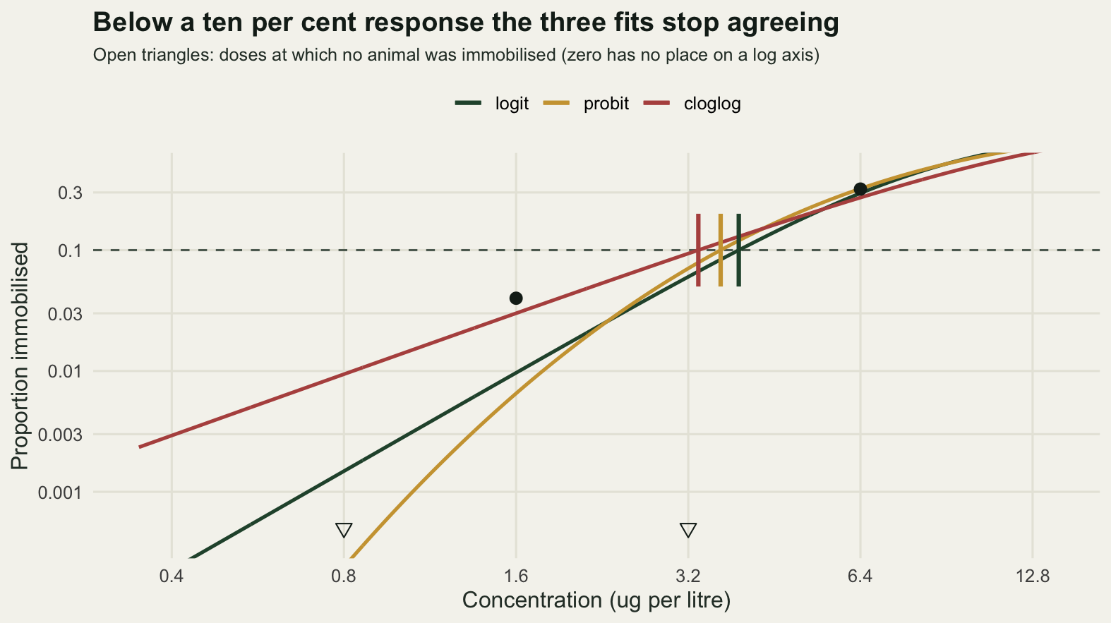
How much of the disagreement is model form and how much is the particular draw? Repeating the experiment 400 times and recording the spread of the three estimates at every level answers it.
set.seed(20260729)
n_spread <- 400
lev_grid <- sort(unique(c(exp(seq(log(0.005), log(0.5), length.out = 40)),
                          0.5, 0.1, 0.05, 0.01)))
sp <- vapply(seq_len(n_spread), function(i) {
  y <- rbinom(length(conc), n_per, true_p(conc, "logit"))
  bs <- lapply(links, function(l) coef(fit_link(y, l)))
  est <- sapply(seq_along(links), function(j)
    exp((link_q(lev_grid, links[j]) - bs[[j]][1]) / bs[[j]][2]))
  apply(est, 1, function(z) max(z) / min(z))
}, numeric(length(lev_grid)))
sp_med <- apply(sp, 1, median)

asym_curve <- sapply(links, function(l)
  exp((link_q(lev_grid, l) - asym_b[[l]][1]) / asym_b[[l]][2]))
sys_all <- apply(asym_curve, 1, function(z) max(z) / min(z))
sys_sym <- apply(asym_curve[, c("logit", "probit")], 1,
                 function(z) max(z) / min(z))

c(datasets = n_spread, warnings_so_far = n_warn)
datasets warnings_so_far
400 23 sel_lev <- c(0.5, 0.1, 0.05, 0.01)
idx <- match(sel_lev, lev_grid)
print(round(rbind(response_level = lev_grid[idx], systematic_all = sys_all[idx],
systematic_symmetric_pair = sys_sym[idx],
median_sampled_all = sp_med[idx]), 4)) [,1] [,2] [,3] [,4]
response_level 0.5000 0.1000 0.0500 0.0100
systematic_all 1.1623 1.2342 1.4666 2.5098
systematic_symmetric_pair 1.0022 1.0592 1.0257 1.1396
median_sampled_all 1.1566 1.1573 1.3491 2.1955The median spread over 400 fresh datasets is 1.1566 at the LC50 and 2.1955 at the LC1, against large-sample values of 1.1623 and 2.5098. Sampling noise is not what makes the links disagree. The disagreement is systematic, it is already there in an infinitely large experiment, and running more animals through the same design does not touch it.
Keeping the two symmetric links apart from the asymmetric one sharpens the picture further. Probit against logit alone spreads 1.0022 at the LC50 and 1.1396 at the LC1, so the symmetric pair never separates far, at any level. The 2.5098 at the LC1 is entirely the price of the tail shape that the complementary log-log link imposes, and that link is the only one of the three that is asymmetric about a response of one half.
lad <- rbind(
  data.frame(p = lev_grid, ratio = sys_all, what = "All three links, large sample"),
  data.frame(p = lev_grid, ratio = sys_sym, what = "Probit against logit, large sample"),
  data.frame(p = lev_grid, ratio = sp_med, what = "All three links, median of 400 datasets"))
lad$what <- factor(lad$what, levels = unique(lad$what))

ggplot(lad, aes(100 * p, ratio, colour = what, linetype = what)) +
  geom_hline(yintercept = 1, colour = te_pal$line, linewidth = 0.8) +
  geom_line(linewidth = 0.9) +
  scale_x_log10(breaks = c(0.5, 1, 2, 5, 10, 20, 50)) +
  scale_colour_manual(values = c(te_pal$clay, te_pal$forest, te_pal$gold), name = NULL) +
  scale_linetype_manual(values = c("solid", "solid", "22"), name = NULL) +
  labs(x = "Response level read off the curve (per cent)",
       y = "Largest estimate divided by smallest",
       title = "The links disagree more the further down the curve you read") +
  theme_te() +
  theme(legend.position = "top", legend.text = element_text(size = 8.5))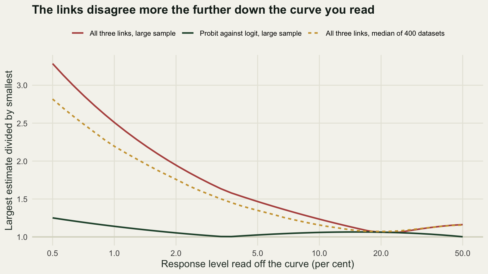
Can the data choose the link?
The obvious reply to all of this is that the link is not an arbitrary choice: fit all three and keep the one the data prefer. The delta-AIC column from the single dataset above already looks thin, so the question is worth a simulation. Draw 300 datasets from each of the three generating links, fit all three links to each, record which one AIC picks, and record what the selected model then says about the LC10 and the LC1.
set.seed(20260729)
n_rep <- 300
sel_mat <- matrix(0, 3, 3, dimnames = list(links, links))
acc <- vector("list", 3); names(acc) <- links
gap_true <- numeric(0); all_close <- 0
for (tl in links) {
  store <- array(NA_real_, c(n_rep, 4, 2),
                 dimnames = list(NULL, c(links, "aic"), c("lc10", "lc1")))
  for (i in seq_len(n_rep)) {
    y <- rbinom(length(conc), n_per, true_p(conc, tl))
    ff <- lapply(links, function(l) fit_link(y, l))
    aa <- sapply(ff, AIC)
    k <- which.min(aa)
    sel_mat[tl, k] <- sel_mat[tl, k] + 1
    all_close <- all_close + (max(aa) - min(aa) < 2)
    if (tl == "logit") gap_true <- c(gap_true, aa[1] - min(aa))
    for (nm in c("lc10", "lc1")) {
      pp <- if (nm == "lc10") 0.1 else 0.01
      est <- sapply(seq_along(links), function(j) lc_hat(ff[[j]], pp, links[j]))
      store[i, , nm] <- c(est, est[k]) / true_lc(pp, tl)
    }
  }
  acc[[tl]] <- store
}
c(datasets_per_truth = n_rep, warnings_total = n_warn)
datasets_per_truth warnings_total
300 161 print(round(sel_mat / n_rep, 4)) logit probit cloglog
logit 0.3567 0.4200 0.2233
probit 0.2233 0.5800 0.1967
cloglog 0.0467 0.1567 0.7967round(c(correct_link_rate = sum(diag(sel_mat)) / (3 * n_rep), chance_rate = 1 / 3,
all_three_within_2_aic = all_close / (3 * n_rep),
median_aic_gap_of_true_link = median(gap_true)), 4) correct_link_rate chance_rate
0.5778 0.3333
all_three_within_2_aic median_aic_gap_of_true_link
0.3100 0.4524 rmse_log <- function(z) sqrt(mean(log(z)^2))
for (nm in c("lc10", "lc1")) {
cat("--", nm, "-- ratio of the estimate to the truth\n")
print(round(rbind(
median_logit_truth = apply(acc[["logit"]][, , nm], 2, median),
median_probit_truth = apply(acc[["probit"]][, , nm], 2, median),
median_cloglog_truth = apply(acc[["cloglog"]][, , nm], 2, median),
rmse_log_logit_truth = apply(acc[["logit"]][, , nm], 2, rmse_log),
rmse_log_probit_truth = apply(acc[["probit"]][, , nm], 2, rmse_log),
rmse_log_cloglog_truth = apply(acc[["cloglog"]][, , nm], 2, rmse_log)), 4))
}-- lc10 -- ratio of the estimate to the truth
logit probit cloglog aic
median_logit_truth 1.0145 0.9656 0.8722 0.9914
median_probit_truth 1.0539 1.0103 0.9327 1.0286
median_cloglog_truth 1.0844 0.9982 1.0228 1.0428
rmse_log_logit_truth 0.1628 0.1703 0.2613 0.1680
rmse_log_probit_truth 0.1558 0.1492 0.1951 0.1512
rmse_log_cloglog_truth 0.1984 0.1951 0.1930 0.1966
-- lc1 -- ratio of the estimate to the truth
logit probit cloglog aic
median_logit_truth 1.0339 1.1835 0.5388 1.0744
median_probit_truth 0.9180 1.0296 0.5162 0.9476
median_cloglog_truth 1.5745 1.7314 1.0784 1.1974
rmse_log_logit_truth 0.2875 0.3118 0.7948 0.3687
rmse_log_probit_truth 0.2609 0.2277 0.7465 0.2982
rmse_log_cloglog_truth 0.5563 0.6447 0.3739 0.4784AIC identifies the generating link in 0.5778 of these experiments, against a chance rate of 0.3333. That is genuinely better than guessing, and it is not the folk claim that model selection is useless here, so it stands. The confusion matrix says where the ability comes from and where it does not. Under a complementary log-log truth AIC finds the complementary log-log link 0.7967 of the time. Under a logit truth it picks the probit 0.4200 of the time and the logit itself only 0.3567: on data generated by a logit, AIC prefers the wrong symmetric link more often than the right one. All three fits land within 2 AIC units of each other in 0.3100 of the experiments, and under a logit truth the median amount by which the true link trails the best is 0.4524, which is nothing.
What that costs depends entirely on which level is being read. At the LC10, under the logit truth, the root mean square error on the log scale is 0.1628 for the correct link, 0.1703 for the probit and 0.2613 for the complementary log-log, and the AIC-selected estimate scores 0.1680. Selecting by AIC is therefore about as accurate as knowing the answer, despite recovering the true link in only 0.3567 of the logit-truth experiments, because the confusion it usually makes is between two links whose LC10 values sit close together anyway. That is a friendlier result than the design of this experiment led me to expect.
At the LC1 the arithmetic turns. The same comparison gives 0.2875 for the correct link, 0.3118 for the probit, 0.7948 for the complementary log-log and 0.3687 for the AIC-selected estimate, so selection is now measurably worse than knowing the link, 0.3687 against 0.2875. The medians say why the error is not just noise: under a logit truth the complementary log-log fit has a median LC1 of 0.5388 times the true value, and under a complementary log-log truth the logit fit has a median LC1 of 1.5745 times the true value. Those are biases, in opposite directions, and they do not average out over a regulatory dossier.
sel_df <- data.frame(truth = factor(rep(links, 3), levels = links),
                     chosen = factor(rep(links, each = 3), levels = links),
                     freq = as.vector(sel_mat / n_rep))
levels(sel_df$truth) <- paste("Generated with", links)

ggplot(sel_df, aes(chosen, freq, fill = chosen)) +
  geom_col(width = 0.68) +
  geom_hline(yintercept = 1 / 3, linetype = "dashed", colour = "#5d6b61") +
  facet_wrap(~truth) +
  scale_fill_manual(values = link_cols, guide = "none") +
  labs(x = "Link chosen by AIC", y = "Frequency over 300 experiments",
       title = "AIC spots the asymmetric link and misses the symmetric pair") +
  theme_te() +
  theme(strip.text = element_text(colour = te_pal$ink, face = "bold"))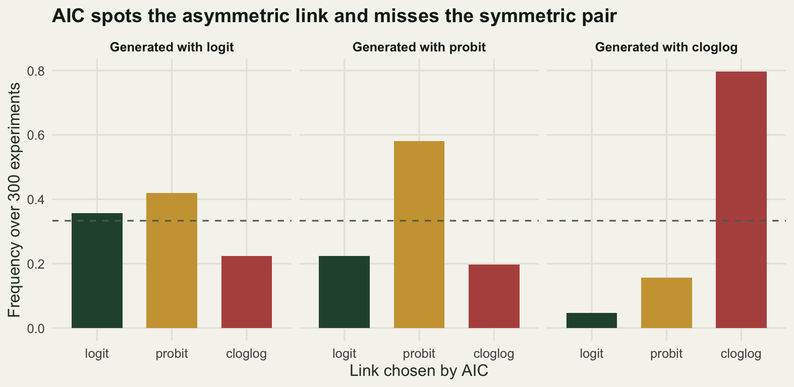
Two strains, one slope, and an exact ratio
What a resistance study reports is not an LC50 but a ratio of two of them, one strain against another. The fit behind that ratio is older than the GLM: put both strains in one model, force a single slope, and read the ratio off the gap between the two intercepts. Finney’s probit analysis calls it a parallel line assay, and the usual defence of the shared slope is that it is steadier than two free ones. On a ladder built the way a range-finding test builds it, something much stronger than steadiness is true, and it is worth separating from the part that is only a hope.
Each strain gets its own doubling series of seven concentrations with twenty-five animals at each, centred on that strain’s own LC50, which is what a range-finder is for. The resistant strain is given an LC50 four times the susceptible one, and the two true slopes are allowed to differ, which is the case a shared slope gets wrong.
cs_rr   <- 4                       # true ratio of the two LC50s
cs_b_s  <- slope_of("logit")       # susceptible slope, per natural log unit
cs_step <- log(2)                  # one rung of the ladder
cs_lev  <- 0.1                     # the low-effect level read off the curve

cs_design <- function(b_r, k = length(conc), step = cs_step, n_dose = n_per,
                      shift = 0, link = "logit") {
  rung <- step * (seq_len(k) - (k + 1) / 2)
  mid  <- rep(c(log(lc50_true), log(lc50_true * cs_rr)), each = k)
  logx <- c(log(lc50_true) + rung, log(lc50_true * cs_rr) + shift + rung)
  is_r <- rep(c(0, 1), each = k)
  list(logx = logx, n = rep(n_dose, 2 * k), link = link, b_s = cs_b_s, b_r = b_r,
       p = link_p(rep(c(cs_b_s, b_r), each = k) * (logx - mid), link),
       xc = cbind(1, is_r, logx), xs = cbind(1, is_r, logx, is_r * logx))
}
cs_true_lr <- function(de, p)        # true log ratio of the level-p doses
  log(cs_rr) + link_q(p, de$link) * (1 / de$b_r - 1 / de$b_s)
cs_pars <- function(de, y, separate) {
  co <- unname(coef(glm.fit(if (separate) de$xs else de$xc, y, weights = de$n,
                            family = binomial(link = de$link))))
  b_lo <- co[3]; b_hi <- if (separate) co[3] + co[4] else co[3]
  q0 <- link_q(0.5, de$link)
  c(m_s = (q0 - co[1]) / b_lo, m_r = (q0 - co[1] - co[2]) / b_hi,
    b_s = b_lo, b_r = b_hi)
}
cs_lr <- function(v, p, link) {      # fitted log ratio at level p
  q <- link_q(p, link)
  (v[["m_r"]] + q / v[["b_r"]]) - (v[["m_s"]] + q / v[["b_s"]])
}
# expected proportions are not counts, so the binomial warning is expected here
cs_large <- function(de) suppressWarnings(cs_pars(de, de$p, FALSE))
cs_held <- function(de, b_fix) {     # the ratio with the common slope held fixed
  co <- unname(coef(suppressWarnings(
    glm.fit(de$xc[, 1:2], de$p, weights = de$n, offset = b_fix * de$logx,
            family = binomial(link = de$link)))))
  -co[2] / b_fix
}

cs_pair   <- cs_design(0.5 * cs_b_s)
cs_held_b <- c(0.3, 0.8, 1.5, 2.6, 6, 12)
cs_any    <- max(abs(sapply(cs_held_b, function(b) cs_held(cs_pair, b)) - log(cs_rr)))
cs_joint  <- cs_large(cs_pair)
cs_exact  <- exp(cs_lr(cs_joint, 0.5, "logit"))
print(c(true_ratio = cs_rr, susceptible_slope = cs_b_s,
        resistant_slope = cs_pair$b_r, fitted_common_slope = cs_joint[["b_s"]]))
true_ratio susceptible_slope resistant_slope fitted_common_slope
4.000000 2.600000 1.300000 1.718169 cat("ratio from the common-slope fit:", sprintf("%.12f", cs_exact), "\n")ratio from the common-slope fit: 4.000000000000 cat("largest log-ratio error with the slope held from",
paste(range(cs_held_b), collapse = " to "), ":",
formatC(cs_any, format = "e", digits = 1), "\n")largest log-ratio error with the slope held from 0.3 to 12 : 1.6e-11 cs_by_link <- sapply(links, function(l)
exp(cs_lr(cs_large(cs_design(0.5 * cs_b_s, link = l)), 0.5, l)))
print(round(cs_by_link, 6)) logit probit cloglog
4.00000 4.00000 3.80734 The LC50 ratio comes back exactly, and that is algebra rather than luck. The algebra needs both ladders, each centred on its own strain; one shared dose series scored on both strains, which is what a laboratory runs before it knows the ratio, does not have it, and the end of this section prices what that costs. Take the fit evaluated at one strain’s true LC50. One rung above the centre the fitted curve misses the truth by exactly what it misses one rung below, with the opposite sign, because the logit is symmetric about a response of one half and the rungs are symmetric about the centre. The score equation for that strain’s intercept adds those misses up, so it is satisfied at the true LC50 whatever slope the fit happens to be carrying. Both strains are in that position at once, which leaves the slope equation one number to fix, and it fixes it between the two true slopes: 1.7182 for true slopes of 2.6 and 1.3. Hold the common slope by hand anywhere from 0.3 to 12 instead of estimating it and the recovered ratio does not move, to 1.6e-11 on the log scale. Estimate it and the ratio is 4.000000000000 against a true 4.
Symmetry is doing the work, not parallelism, and the earlier sections have already said which links have it. The same expected responses fitted through the probit give 4.000000, and through the complementary log-log, the one link of the three that is not symmetric about a response of one half, they give 3.8073. Whatever makes the probit and the logit agree at the LC50 of one strain is what makes a parallel line assay exact for two. Noise does not spoil it either, by the same route: reversing the order of the doses within a strain and replacing each count by the number of animals left moving gives an experiment with exactly the same distribution and exactly the opposite error in the fitted log ratio, so that error is symmetric about zero at any number of animals, not only in a large experiment.
None of it survives the trip down the curve, and the way it fails is a formula rather than a simulation. A common-slope fit reports one ratio and reports it at every level, since the gap between the intercepts divided by the shared slope does not depend on where the curve is read. The truth does depend on where it is read, because two curves with different slopes separate as they leave one half. The error of the common-slope ratio at level p is exp(-logit(p) (1 / b_R - 1 / b_S)), with b_R and b_S the two true slopes, and there is nothing else in it: not the fitted common slope, not the spacing of the ladder, not the number of animals.
cs_grid  <- c(1, 0.85, 0.7, 0.5, 0.25)
cs_steep <- c(1.3, 2, 4)
cs_closed <- t(sapply(c(cs_grid, cs_steep), function(rho) {
  de <- cs_design(rho * cs_b_s)
  c(slope_ratio = rho,
    measured = exp(cs_lr(cs_large(de), cs_lev, "logit") - cs_true_lr(de, cs_lev)),
    closed_form = exp(-link_q(cs_lev, "logit") * (1 / de$b_r - 1 / de$b_s)))
}))
print(round(cs_closed, 6))
slope_ratio measured closed_form
[1,] 1.00 1.000000 1.000000
[2,] 0.85 1.160827 1.160827
[3,] 0.70 1.436457 1.436457
[4,] 0.50 2.328179 2.328179
[5,] 0.25 12.619701 12.619701
[6,] 1.30 0.822818 0.822818
[7,] 2.00 0.655378 0.655378
[8,] 4.00 0.530564 0.530564cat("largest gap between the two columns:",
formatC(max(abs(cs_closed[, "measured"] - cs_closed[, "closed_form"])),
format = "e", digits = 1), "\n")largest gap between the two columns: 1.1e-15 cs_floor <- exp(link_q(cs_lev, "logit") / cs_b_s)
cs_off <- t(sapply(c(0, 0.5, 1), function(s) {
de <- cs_design(0.5 * cs_b_s, shift = s * cs_step)
c(ladder_off_by_rungs = s, ratio = exp(cs_lr(cs_large(de), 0.5, "logit")))
}))
print(round(cbind(cs_off, bound_for_a_steeper_strain = cs_floor), 6)) ladder_off_by_rungs ratio bound_for_a_steeper_strain
[1,] 0.0 4.000000 0.42952
[2,] 0.5 4.074963 0.42952
[3,] 1.0 4.163938 0.42952At the LC10 with a resistant strain half as steep the factor is 2.3282, and the large-sample fit agrees with the formula to 1.1e-15 across the whole sweep. The two directions are not each other’s mirror. A flatter resistant strain sends the factor up without limit, already 12.62 by the time its slope is a quarter of the susceptible one, while a steeper resistant strain can never pull the LC10 ratio below 0.4295 of the truth however steep it gets. Exactness at the LC50 is also the one thing an off-centre ladder costs: put the resistant series a whole doubling away from that strain’s LC50, which is an ordinary outcome of a range-finding test, and the recovered ratio moves to 4.1639.
That shift moved one arm. The design that gives the exactness up altogether is the one a laboratory runs before it knows the ratio: a single series of concentrations with both strains scored at the same doses, since a range-finding test on the resistant strain is precisely what has not happened yet. Neither arm is then centred on its own LC50, the misses above and below the centre stop cancelling within a strain, and the score equations settle somewhere other than the truth. This is a large-sample question, so the expected responses answer it without a simulation.
# one series of concentrations for both strains, centred where the laboratory
# guessed rather than on each strain's own LC50
cs_shared <- function(rho, centre, k = length(conc), step = cs_step,
                      n_dose = n_per, link = "logit") {
  rung <- step * (seq_len(k) - (k + 1) / 2)
  logx <- rep(log(centre) + rung, 2)
  mid  <- rep(c(log(lc50_true), log(lc50_true * cs_rr)), each = k)
  is_r <- rep(c(0, 1), each = k)
  b_r  <- rho * cs_b_s
  list(logx = logx, n = rep(n_dose, 2 * k), link = link, b_s = cs_b_s, b_r = b_r,
       p = link_p(rep(c(cs_b_s, b_r), each = k) * (logx - mid), link),
       xc = cbind(1, is_r, logx), xs = cbind(1, is_r, logx, is_r * logx))
}
cs_err <- function(de, separate = FALSE)   # per cent error of the fitted LC50 ratio
  100 * (exp(cs_lr(suppressWarnings(cs_pars(de, de$p, separate)), 0.5, de$link)) /
           cs_rr - 1)
cs_centre <- c(geometric_mean = lc50_true * sqrt(cs_rr), susceptible = lc50_true)

cs_one <- t(sapply(cs_grid, function(rho) c(
  slope_ratio = rho,
  sapply(cs_centre, function(cc) cs_err(cs_shared(rho, cc))),
  own_centred = cs_err(cs_design(rho * cs_b_s)),
  free_slopes = max(abs(sapply(cs_centre, function(cc)
    cs_err(cs_shared(rho, cc), TRUE)))))))
print(round(cs_one[, c("slope_ratio", "geometric_mean", "susceptible",
                       "own_centred")], 3))
slope_ratio geometric_mean susceptible own_centred
[1,] 1.00 0.000 0.000 0
[2,] 0.85 -0.054 -1.138 0
[3,] 0.70 -0.331 -3.412 0
[4,] 0.50 -1.662 -10.137 0
[5,] 0.25 -7.515 -32.127 0cat("largest error with two free slopes on the same shared series:",
formatC(max(cs_one[, "free_slopes"]), format = "e", digits = 1), "\n")largest error with two free slopes on the same shared series: 1.1e-10 The columns are per cent errors of the recovered LC50 ratio. Put the shared series at the geometric mean of the two true LC50s, which is the best a single ladder can do, and the ratio comes back short by 1.66 per cent when the resistant strain is half as steep and by 7.51 per cent when it is a quarter as steep. Centre the same series on the susceptible strain, which is what happens when the resistance is the surprise, and those two become 10.14 and 32.13 per cent. The second of those is several times what the one-doubling shift above costs, and in the other direction. Equal slopes still come back exactly wherever the shared ladder sits, because the common-slope model is then the true model and there is nothing for the centring to rescue. Two free slopes are exact on the shared series as well, to 1.1e-10, which places the loss where it belongs: the shared series does not spoil the data, it removes the cancellation that was making the constrained fit right. The exactness is a property of the two ladders, not of the parallel line assay, and a resistance ratio read off one shared dose series has not inherited it.
An exact LC50 and a known bias elsewhere still do not say which fit to use, because the separate fit pays for its extra slope in variance. That is a measurement rather than an argument, so here it is: 2000 simulated pairs of strains at each slope pair, root mean square error of the log ratio, common slope against separate slopes, with a paired bootstrap standard error on every comparison. The table holds the animals at twenty-five per dose; the same sweep at other numbers is used further down.
cs_rms <- function(z) sqrt(mean(z^2))
cs_se <- function(a, b, n_boot = 800) {
  idx <- matrix(sample.int(length(a), length(a) * n_boot, TRUE), n_boot)
  sd(apply(idx, 1, function(i) cs_rms(a[i]) / cs_rms(b[i])))
}
cs_warn <- 0; cs_fits <- 0
cs_mc <- function(rho, n_rep = 2000, ...) {
  de <- cs_design(rho * cs_b_s, ...)
  set.seed(20260729)
  cs_fits <<- cs_fits + 2 * n_rep
  seen <- cs_warn
  err <- t(vapply(seq_len(n_rep), function(i) {
    y <- rbinom(length(de$p), de$n, de$p) / de$n
    fit <- withCallingHandlers(
      list(cs_pars(de, y, FALSE), cs_pars(de, y, TRUE)),
      warning = function(w) { cs_warn <<- cs_warn + 1; invokeRestart("muffleWarning") })
    c(cs_lr(fit[[1]], 0.5, de$link) - cs_true_lr(de, 0.5),
      cs_lr(fit[[2]], 0.5, de$link) - cs_true_lr(de, 0.5),
      cs_lr(fit[[1]], cs_lev, de$link) - cs_true_lr(de, cs_lev),
      cs_lr(fit[[2]], cs_lev, de$link) - cs_true_lr(de, cs_lev))
  }, numeric(4)))
  c(slope_ratio = rho,
    bias_factor = exp(-link_q(cs_lev, "logit") * (1 / de$b_r - 1 / de$b_s)),
    animals_per_dose = de$n[1],
    rmse_common_50 = cs_rms(err[, 1]), rmse_separate_50 = cs_rms(err[, 2]),
    ratio_50 = cs_rms(err[, 1]) / cs_rms(err[, 2]),
    mc_se_50 = cs_se(err[, 1], err[, 2]),
    rmse_common_10 = cs_rms(err[, 3]), rmse_separate_10 = cs_rms(err[, 4]),
    ratio_10 = cs_rms(err[, 3]) / cs_rms(err[, 4]),
    mc_se_10 = cs_se(err[, 3], err[, 4]),
    median_error_50 = median(err[, 1]), exact_hits = mean(abs(err[, 1]) < 1e-12),
    worst_share_10 = sum(sort(err[, 4]^2, decreasing = TRUE)[seq_len(n_rep / 100)]) /
      sum(err[, 4]^2),
    warned_fits = cs_warn - seen)
}
cs_by_n <- do.call(rbind, lapply(c(10, n_per, 100), function(nd)
  t(sapply(cs_grid, cs_mc, n_dose = nd))))
cs_corner <- cs_by_n[cs_by_n[, "animals_per_dose"] == 10 &
                     cs_by_n[, "slope_ratio"] == min(cs_grid), ]
cs_main <- rbind(cs_by_n[cs_by_n[, "animals_per_dose"] == n_per, ],
                 t(sapply(cs_steep, cs_mc)))
rownames(cs_main) <- c("equal", "mild", "moderate", "strong", "extreme",
                       "steep_mild", "steep_strong", "steep_extreme")
print(round(cs_main[, c("slope_ratio", "rmse_common_50", "rmse_separate_50",
                        "ratio_50", "mc_se_50", "median_error_50",
                        "exact_hits")], 4))
slope_ratio rmse_common_50 rmse_separate_50 ratio_50 mc_se_50
equal 1.00 0.1483 0.1482 1.0004 0.0001
mild 0.85 0.1549 0.1550 0.9993 0.0002
moderate 0.70 0.1643 0.1650 0.9955 0.0004
strong 0.50 0.1810 0.1863 0.9715 0.0012
extreme 0.25 0.2214 0.2811 0.7876 0.0050
steep_mild 1.30 0.1393 0.1386 1.0051 0.0010
steep_strong 2.00 0.1297 0.1235 1.0502 0.0048
steep_extreme 4.00 0.1249 0.1069 1.1688 0.0115
median_error_50 exact_hits
equal 0 0.0660
mild 0 0.0565
moderate 0 0.0540
strong 0 0.0560
extreme 0 0.0545
steep_mild 0 0.0600
steep_strong 0 0.0550
steep_extreme 0 0.0695print(round(cs_main[, c("bias_factor", "rmse_common_10", "rmse_separate_10",
"ratio_10", "mc_se_10", "warned_fits")], 4)) bias_factor rmse_common_10 rmse_separate_10 ratio_10 mc_se_10
equal 1.0000 0.1483 0.2417 0.6134 0.0106
mild 1.1608 0.2137 0.2565 0.8331 0.0156
moderate 1.4365 0.3956 0.2767 1.4297 0.0244
strong 2.3282 0.8625 0.3416 2.5253 0.0412
extreme 12.6197 2.5417 0.8326 3.0527 0.0717
steep_mild 0.8228 0.2409 0.2289 1.0520 0.0191
steep_strong 0.6554 0.4430 0.2600 1.7039 0.0266
steep_extreme 0.5306 0.6472 0.2101 3.0801 0.0489
warned_fits
equal 0
mild 0
moderate 0
strong 0
extreme 0
steep_mild 18
steep_strong 505
steep_extreme 1927c(fits_made = cs_fits, fits_with_a_warning = cs_warn) fits_made fits_with_a_warning
72000 2760 At the LC50 the shared slope buys nothing at all. With the two slopes equal, the one case where the common-slope model is not even wrong, the error ratio is 1.0004 with a standard error of 0.0001, and spending the extra parameter costs nothing measurable either, because on a ladder centred where this one is centred the LC50 and the slope are estimated almost independently of one another. What the shared slope buys is at the LC10, where the same comparison reads 0.6134, an error smaller by nearly two fifths for free. The median of the error in the common-slope ratio at the LC50 is 0 in every row of the sweep, which is the reflection argument showing up in a histogram. In 5.9 per cent of the experiments the two strains recorded the same total of immobilised animals, which pools both arms onto one curve in rung coordinates, and the estimate hit the truth to machine precision.
Push the slope difference to both ends and the ordering reverses, differently at the two levels. At the LC10 it reverses with the size of the difference: the common-slope fit is ahead at 0.8331 when the resistant slope is 0.85 of the susceptible one, has lost that advantage by the time the resistant slope is 0.7 of it, where the comparison reads 1.4297, and is behind by a factor of 3.0527 at a slope ratio of 0.25. On the other side the crossing comes sooner, at 1.052 for a slope ratio of only 1.3. At the LC50 the ordering reverses with the direction instead: the common-slope fit is better, at 0.7876, when the resistant strain is the flatter one, because a flat strain’s own slope is badly determined and pooling rescues it, and worse, at 1.1688, when the resistant strain is the steeper one, because pooling then drags a well-determined slope down. Both of those sit many standard errors from one.
Every number in that table is conditional on four choices that were never varied: seven doses per strain, one doubling between rungs, twenty-five animals at each, and a ladder centred on the truth. Free them one at a time.
cs_free <- rbind(
  cs_by_n[cs_by_n[, "slope_ratio"] == 0.85, ],
  cs_mc(0.85, k = 5), cs_mc(0.85, k = 11),
  cs_mc(0.85, step = log(1.5)), cs_mc(0.85, step = log(3)),
  cs_mc(0.85, shift = cs_step),
  cs_mc(0.7, n_dose = 10), cs_mc(0.7, n_dose = 100))
rownames(cs_free) <- c("animals_few", "animals_base", "animals_many",
                       "doses_few", "doses_many", "spacing_narrow",
                       "spacing_wide", "ladder_off", "wider_gap_few",
                       "wider_gap_many")
print(round(cs_free[, c("slope_ratio", "animals_per_dose", "ratio_50", "mc_se_50",
                        "ratio_10", "mc_se_10", "median_error_50",
                        "warned_fits")], 4))
slope_ratio animals_per_dose ratio_50 mc_se_50 ratio_10 mc_se_10
animals_few 0.85 10 1.0020 0.0019 0.6761 0.0141
animals_base 0.85 25 0.9993 0.0002 0.8331 0.0156
animals_many 0.85 100 0.9994 0.0001 1.3437 0.0241
doses_few 0.85 25 0.9971 0.0005 0.8091 0.0168
doses_many 0.85 25 1.0004 0.0001 0.8554 0.0151
spacing_narrow 0.85 25 0.9938 0.0008 0.8479 0.0158
spacing_wide 0.85 25 1.0163 0.0026 0.6893 0.0145
ladder_off 0.85 25 0.9983 0.0009 0.8513 0.0160
wider_gap_few 0.70 10 0.9957 0.0016 0.9734 0.0188
wider_gap_many 0.70 100 0.9957 0.0002 2.7513 0.0461
median_error_50 warned_fits
animals_few 0.0000 66
animals_base 0.0000 0
animals_many 0.0000 0
doses_few 0.0000 0
doses_many 0.0000 0
spacing_narrow 0.0000 0
spacing_wide 0.0000 123
ladder_off 0.0046 0
wider_gap_few 0.0000 51
wider_gap_many 0.0000 0c(fits_made = cs_fits, fits_with_a_warning = cs_warn) fits_made fits_with_a_warning
100000 2934 Only one of the four moves the answer, and it is the one nobody files under model choice. Hold the strains at a slope ratio of 0.85 and change nothing but the number of animals: at the LC10 the common-slope fit is ahead by 0.6761 with 10 animals per dose, still ahead at 0.8331 with 25, and behind at 1.3437 with 100. The same two strains, the same systematic error, the opposite recommendation, because the bias is fixed while the noise it competes against shrinks with the animals. A wider slope gap does the same thing: at a slope ratio of 0.7 the comparison runs from 0.9734 to 2.7513 over the same range of animals. Doses per strain matter less, 0.8091 against 0.8554 for five rungs against eleven. Spacing matters a little, in the direction that a wider ladder leaves less of the design near the LC50, so the free slopes get noisier and pooling looks better: 0.6893 for a threefold ladder. The off-centre ladder is the interesting one, because it leaves the LC10 comparison where it was, at 0.8513, and takes away the thing that made the LC50 worth having: the median of the error there is 0.0046 rather than zero.
cs_df <- data.frame(slope_ratio = cs_by_n[, "slope_ratio"],
                    ratio = cs_by_n[, "ratio_10"], se = cs_by_n[, "mc_se_10"],
                    animals = factor(cs_by_n[, "animals_per_dose"]))

ggplot(cs_df, aes(slope_ratio, ratio, colour = animals)) +
  geom_hline(yintercept = 1, colour = te_pal$line, linewidth = 0.8) +
  geom_errorbar(aes(ymin = ratio - se, ymax = ratio + se), width = 0.03,
                linewidth = 0.6) +
  geom_line(linewidth = 0.9) +
  geom_point(size = 2) +
  scale_x_log10(breaks = cs_grid) +
  scale_y_log10(breaks = c(0.5, 0.7, 1, 1.5, 2, 3, 5)) +
  scale_colour_manual(values = c(te_pal$forest, te_pal$gold, te_pal$clay),
                      name = "animals per dose") +
  labs(x = "Resistant slope divided by susceptible slope",
       y = "Common-slope error divided by separate-slope error",
       title = "Where a shared slope stops paying at the LC10",
       subtitle = paste("Above the line the extra parameter is worth buying;",
                        "bars are one bootstrap standard error")) +
  theme_te() +
  theme(legend.position = "top",
        plot.subtitle = element_text(size = 9.5, colour = "#2c3a31"))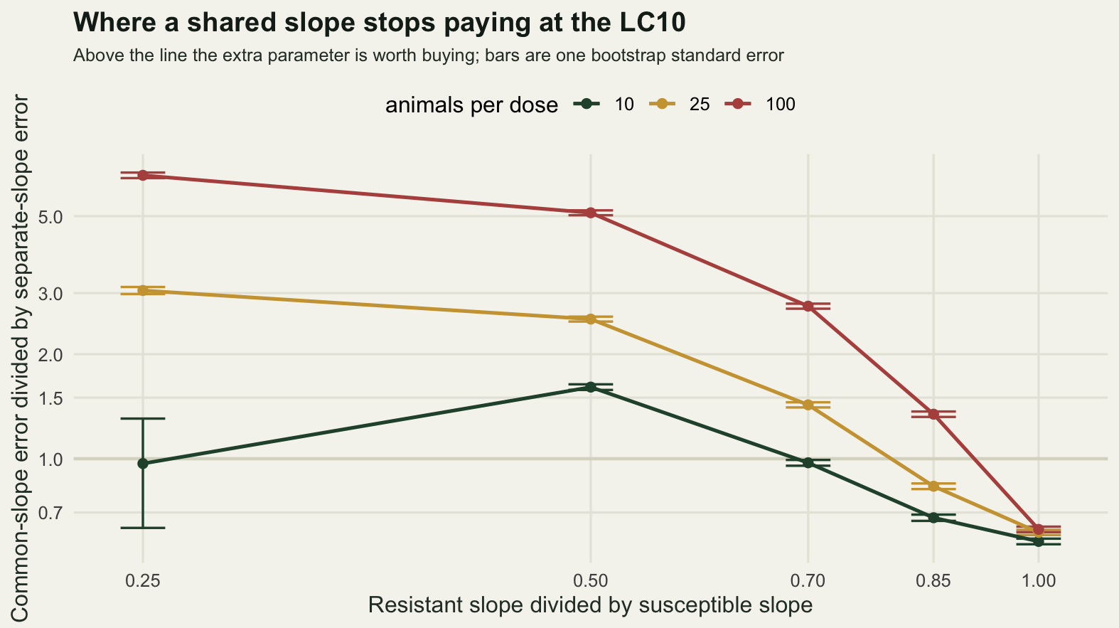
The leftmost point of the ten-animal line is the honest hole in the picture. Its standard error is 0.3366, several times any other in the sweep, because with 10 animals and a resistant curve a quarter as steep the separate fit occasionally fails outright: the worst one per cent of its experiments carry 72 per cent of its total squared error. Which fit wins in that corner is not resolved by 2000 replicates, and no sentence here should pretend otherwise. The warnings counted in the chunks above are all of one kind, fitted probabilities numerically zero or one, and the last column of the sweep says where they live: 1927 of them in the steepest pair, and none at all in any twenty-five animal row where the resistant strain is the flatter one.
So the shared slope is the right choice more often than its reputation as a convenience suggests, and for a reason that has nothing to do with parsimony. If the number wanted is a ratio of LC50s and each ladder is centred on its own strain, the common-slope fit is exact whatever the slopes do, which no amount of extra parameters can improve on. If the number wanted is a low-effect ratio, the shared slope is the better estimator over most of the window where the closed-form factor stays inside roughly 0.82 to 1.16, though the two edges of that window are not alike. At the flatter edge it is still well ahead, 0.8331 against the separate fit, while at the steeper edge it has already slipped behind, at 1.052 with a standard error of 0.0191, so the window as drawn is a little wider than the region where the shared slope actually wins. The smaller the experiment the wider that window gets. What it cannot do is make a single resistance ratio exist when the slopes genuinely differ. Two curves that are not parallel stand in a different ratio at every level, so a parallel line assay run on them answers at the LC50 and reports the answer as though the level had not been chosen. That is a choice dressed as a summary, and the formula above says exactly what it costs.
The honest limit
Two of the numbers above deserve to be put side by side. At the LC10 the sampling interval spans a factor of 1.9901 while the three links disagree by 1.2342, so on this design the animals are still the dominant source of uncertainty. At the LC1 the interval spans 3.3890 and the links disagree by 2.5098, which is much closer. The difference between the two sources is that one of them shrinks when you buy more animals and the other does not.
n_now <- length(conc) * n_per
round(c(animals_now = n_now,
        animals_for_lc10_parity =
          n_now * (log(median(cal[, "wid10"])) / log(sys_all[idx[2]]))^2,
        animals_for_lc1_parity =
          n_now * (log(median(cal[, "wid1"])) / log(sys_all[idx[4]]))^2), 1)
animals_now animals_for_lc10_parity animals_for_lc1_parity
175.0 1872.6 307.9 Treating the interval width as scaling with the square root of the number of animals, the two sources reach parity at about 1872.6 animals for the LC10 and about 307.9 animals for the LC1. The comparison is crude, since an interval width and a spread between three point estimates are not the same object, but the scale is the point: at the LC1 an experiment less than twice the size of this one is already limited by a choice the analyst makes rather than by the animals. Reporting a confidence interval from one link, at that level, understates the uncertainty by a factor that no amount of extra testing will remove.
Three further limits sit outside what was measured here. The generating curve was itself one of the three links under test, which is generous: a real dose-response surface has no reason to be exactly probit, logit or complementary log-log, so the spread measured above is a lower bound on model-form uncertainty rather than an estimate of it. The animals were treated as independent binomial trials, which they are not when they share a vessel, and vessel-level clustering makes every interval here too narrow. And the concentrations were assumed to be known exactly and the control mortality to be zero. Those three assumptions are the subject of Checking a dose-response analysis, and each of them moves the low-effect end of the curve more than the middle, in the same direction as everything measured here.
Where to go next
The intervals in this post were built with Fieller’s theorem and checked once for coverage, which is enough to establish that the estimates are calibrated but not enough to choose an interval method. Confidence intervals for effective doses takes that apart properly, including the design question this post left alone: where to place the concentrations if the low-effect end is what the report will quote.
Two other directions lead out of the same fit. Everything above assumes the response rises monotonically with concentration, and Hormesis and non-monotonic responses measures what a monotone model does to an effective dose when the data carry a low-dose stimulation instead. And the curves here were fitted as generalised linear models because a link function made that possible; when the shape needs an asymptote or an extra parameter, the fit becomes a nonlinear least squares or likelihood problem of the kind in Nonlinear regression with nls.
References
Ritz C 2010 Environmental Toxicology and Chemistry 29(1):220-229 (10.1002/etc.7)
Ritz C, Baty F, Streibig JC, Gerhard D 2015 PLOS ONE 10(12):e0146021 (10.1371/journal.pone.0146021)
Fieller EC 1954 Journal of the Royal Statistical Society Series B 16(2):175-185 (10.1111/j.2517-6161.1954.tb00159.x)
Finney DJ 1971 Probit Analysis. 3rd edition. Cambridge University Press, ISBN 978-0-521-08041-5
Collett D 2003 Modelling Binary Data. 2nd edition. Chapman and Hall/CRC, ISBN 978-1-58488-324-1