library(ggplot2)

te_pal <- list(forest = "#275139", green = "#2f8f63", sage = "#93a87f",
               clay = "#b5534e", gold = "#cda23f", line = "#dad9ca",
               ink = "#16241d", paper = "#f5f4ee")

theme_te <- function() {
  theme_minimal(base_size = 12) +
    theme(panel.grid.minor = element_blank(),
          panel.grid.major = element_line(colour = "#e7e6dc"),
          plot.background = element_rect(fill = "#f5f4ee", colour = NA),
          panel.background = element_rect(fill = "#f5f4ee", colour = NA),
          plot.title = element_text(face = "bold", colour = te_pal$ink),
          axis.title = element_text(colour = "#2c3a31"))
}Checking a dose-response analysis
R
ecotoxicology
GLM
ecology tutorial
ggplot2
Five checks on an ecotoxicology dose-response fit in R: control mortality, vessel overdispersion, tail extrapolation, nominal dose, and the two-stressor null.
A 96 hour acute test finishes, the counts go into a spreadsheet, and a curve comes back with an LC50 of 12 micrograms per litre and a confidence interval that spans about a third of that either way. The number goes into a risk assessment and stops being a statistic. What nobody looks at again is the set of assumptions that turned twelve columns of dead and alive into a single quantile: that the control animals died for reasons the model does not need to know about, that each animal is an independent draw, that the curve keeps its shape below the lowest concentration anyone tested, and that the concentration written on the beaker is the concentration the animals were in.
The three earlier posts in this cluster build the machinery. Dose-response curves and the LC50 fits the curve and shows that the LC50 is a fitted quantity rather than a measurement. Confidence intervals for effective doses prices the uncertainty around it and shows where the design decides the answer. Hormesis and non-monotonic responses asks whether the curve is monotone at all. This post tries to break all three by measuring what four common defects do to the fitted number: how far the LC50 moves, and how far the stated 95 per cent interval is from covering the truth 95 per cent of the time. Every check is a simulation with a known answer, because coverage cannot be measured any other way. A fifth check follows those four and steps outside the single toxicant assay, to the null a two-stressor design is judged against.
The machinery underneath is the binomial GLM from Logistic regression for presence-absence data, with a log concentration axis instead of an environmental gradient. One point of vocabulary before the code: the log-logistic curve used here runs on a dose axis, so the proportion killed rises with concentration. In Parametric survival and the AFT model the same distribution runs on a time axis, where the quantile of interest is a survival time. The algebra is shared and the reported number means something different in each.
The assay under test
The test animal is a small crustacean, the endpoint is death at 96 hours, and the design is the one that appears in every guideline: a control plus five concentrations spaced by a factor of about 1.8, with 25 animals at each level. The truth is a log-logistic curve on the concentration axis with an LC50 of 12 and a slope of 2.2 on the natural log scale, and 8 per cent of animals die during the test whatever the exposure.
Two functions do all the fitting. The two-parameter fit is a binomial GLM of dead out of total on log concentration, with a link that the caller chooses; the effective dose at any level comes from inverting the linear predictor, and its standard error from the delta method on the log dose scale. The three-parameter fit adds a lower asymptote for the control mortality and is done by direct maximum likelihood, with parameters on the log, log and probability scales and the concentration of the control set to zero so that its predicted mortality is the asymptote itself.
p_true <- function(x, b, e, c0) c0 + (1 - c0) * plogis(b * (log(x) - log(e)))

fit2 <- function(x, dead, n, link = "logit") {
  X <- cbind(1, log(x))
  fo <- glm.fit(X, dead / n, weights = n, family = binomial(link))
  list(co = fo$coefficients, V = solve(crossprod(X * sqrt(fo$weights))),
       mu = fo$fitted.values, df = fo$df.residual)
}

lc_of <- function(co, V, p, link = "logit") {
  q <- switch(link, logit = qlogis(p), probit = qnorm(p),
              cloglog = log(-log(1 - p)))
  lx <- (q - co[1]) / co[2]
  gr <- c(-1 / co[2], -lx / co[2])
  c(lx = unname(lx), se = unname(sqrt(drop(gr %*% V %*% gr))))
}

nll3 <- function(par, x, dead, n) {
  bb <- exp(par[1]); le <- par[2]; c0 <- par[3]
  p <- c0 + (1 - c0) * plogis(bb * (log(x) - le))
  p <- pmin(pmax(p, 1e-12), 1 - 1e-12)
  -sum(dead * log(p) + (n - dead) * log(1 - p))
}

fit3 <- function(x, dead, n) {
  st <- c(log(2), log(median(x[x > 0])), max(dead[x == 0] / n[x == 0], 0.02))
  o <- optim(st, nll3, x = x, dead = dead, n = n, method = "L-BFGS-B",
             lower = c(-2, log(0.05), 0.001), upper = c(3, log(2000), 0.6),
             control = list(maxit = 1000, factr = 1e9))
  V <- solve(optimHess(o$par, nll3, x = x, dead = dead, n = n))
  c(lx = o$par[2], se = sqrt(V[2, 2]), c0 = o$par[3], b = exp(o$par[1]),
    conv = o$convergence)
}set.seed(20260801)
b_true <- 2.2; e_true <- 12; c0_true <- 0.08
conc <- c(3.7, 6.7, 12.0, 21.6, 38.9)
n_per <- 25
print(round(c(lc50 = e_true, slope = b_true, control_mortality_pct = 100 * c0_true,
test_hours = 96, animals_per_level = n_per, levels = length(conc),
total_animals = n_per * (length(conc) + 1)), 3)) lc50 slope control_mortality_pct
12.0 2.2 8.0
test_hours animals_per_level levels
96.0 25.0 5.0
total_animals
150.0 print(round(c(spacing_factor = mean(conc[-1] / conc[-length(conc)])), 1))spacing_factor
1.8 print(round(rbind(concentration = conc,
true_mortality = p_true(conc, b_true, e_true, c0_true)), 3)) [,1] [,2] [,3] [,4] [,5]
concentration 3.700 6.70 12.00 21.600 38.900
true_mortality 0.144 0.28 0.54 0.802 0.936d_ctrl <- rbinom(1, n_per, c0_true)
d_trt <- rbinom(length(conc), n_per, p_true(conc, b_true, e_true, c0_true))
print(rbind(dead = c(d_ctrl, d_trt), n = rep(n_per, length(conc) + 1))) [,1] [,2] [,3] [,4] [,5] [,6]
dead 0 4 7 13 20 24
n 25 25 25 25 25 25g0 <- fit2(conc, d_trt, rep(n_per, length(conc)))
print(round(c(naive_lc50 = exp(lc_of(g0$co, g0$V, 0.5)["lx"]),
naive_slope = unname(g0$co[2])), 3))naive_lc50.lx naive_slope
10.395 1.931 The single data set drawn here happens to have no deaths at all in the control, and mortality among the treated groups runs from 4 out of 25 to 24 out of 25. A two-parameter fit that drops the control returns an LC50 of 10.395 against a truth of 12 and a slope of 1.931 against a truth of 2.2, so on this draw a clean control was no guarantee: the background deaths are still sitting inside the treated counts. That is one draw, and one draw proves nothing. The rest of the post is about what happens on average, and about how often the interval contains the truth.
Check 1: control mortality and the Abbott correction
If animals die in the control, the observed mortality at a treated level mixes two processes. The standard repair is Abbott’s correction, which is a century old and still in the guidelines: subtract the control mortality and rescale, so that a proportion p observed at a concentration becomes (p minus c) divided by (1 minus c), where c is the control mortality. The corrected proportions then go into an ordinary two-parameter fit.
The alternative is to write the control mortality into the model as a lower asymptote and estimate it from the same data, which is what the three-parameter fit above does. Both are defensible and both are in common use. The difference is not in the point estimate, and this is the part that is easy to miss: Abbott’s correction treats the control mortality as known exactly. The control group is a sample like any other, its mortality has a standard error of its own, and the corrected proportions inherit that error while the fit that follows knows nothing about it.
Three estimators are compared on 1000 simulated data sets from the design above: the naive fit that drops the control, the Abbott fit, and the three-parameter fit. Each returns an LC50 and a delta method standard error on the log scale, and each is scored on bias and on the coverage of its nominal 95 per cent interval. Abbott’s corrected counts are rounded to whole animals, which is what software does when the corrected proportion has to go back into a binomial fit.
set.seed(20260801)
n_rep <- 1000
nn <- rep(n_per, length(conc))
dc_all <- rbinom(n_rep, n_per, c0_true)
dt_all <- matrix(rbinom(n_rep * length(conc), n_per,
                        rep(p_true(conc, b_true, e_true, c0_true), each = n_rep)),
                 n_rep, length(conc))

res1 <- t(vapply(seq_len(n_rep), function(i) {
  dt <- dt_all[i, ]; chat <- dc_all[i] / n_per
  fn <- fit2(conc, dt, nn)
  a_d <- pmin(pmax(round(((dt / n_per - chat) / (1 - chat)) * n_per), 0), n_per)
  fa <- fit2(conc, a_d, nn)
  fj <- fit3(c(0, conc), c(dc_all[i], dt), rep(n_per, length(conc) + 1))
  c(lc_of(fn$co, fn$V, 0.5), lc_of(fa$co, fa$V, 0.5),
    unname(fj[c("lx", "se", "c0", "conv")]))
}, numeric(8)))
colnames(res1) <- c("naive_lx", "naive_se", "abb_lx", "abb_se",
                    "joint_lx", "joint_se", "joint_c0", "conv")

lt <- log(e_true)
summ1 <- function(lx, se) c(
  median_lc50 = median(exp(lx)),
  bias_pct = 100 * (exp(mean(lx)) / e_true - 1),
  sd_log = sd(lx), mean_se_log = mean(se),
  cover_pct = 100 * mean(abs(lx - lt) < 1.96 * se))
print(round(rbind(naive = summ1(res1[, 1], res1[, 2]),
                  abbott = summ1(res1[, 3], res1[, 4]),
                  joint = summ1(res1[, 5], res1[, 6])), 3))
median_lc50 bias_pct sd_log mean_se_log cover_pct
naive 10.469 -12.380 0.117 0.118 79.9
abbott 11.867 -0.831 0.142 0.106 86.0
joint 11.918 -0.137 0.143 0.140 93.7print(round(c(naive_bias_pct = 100 * (exp(mean(res1[, 1])) / e_true - 1),
abbott_bias_pct = 100 * (exp(mean(res1[, 3])) / e_true - 1),
joint_bias_pct = 100 * (exp(mean(res1[, 5])) / e_true - 1)), 1)) naive_bias_pct abbott_bias_pct joint_bias_pct
-12.4 -0.8 -0.1 print(round(c(replicates = n_rep, nonconvergence = sum(res1[, "conv"] != 0),
zero_control_deaths_pct = 100 * mean(dc_all == 0),
asymptote_at_bound_pct = 100 * mean(res1[, "joint_c0"] <= 0.0011),
se_ratio_abbott = mean(res1[, 4]) / sd(res1[, 3]),
se_ratio_joint = mean(res1[, 6]) / sd(res1[, 5])), 3)) replicates nonconvergence zero_control_deaths_pct
1000.000 0.000 12.200
asymptote_at_bound_pct se_ratio_abbott se_ratio_joint
12.000 0.747 0.981 meth <- c("naive", "Abbott", "three-parameter")
cols <- c(1, 3, 5)
bars <- do.call(rbind, lapply(seq_along(meth), function(i) {
lx <- res1[, cols[i]]; se <- res1[, cols[i] + 1]
qq <- quantile(lx, c(0.025, 0.975))
data.frame(method = meth[i], row = 4 - i,
lo = c(unname(qq[1]), median(lx) - 1.96 * mean(se)),
hi = c(unname(qq[2]), median(lx) + 1.96 * mean(se)),
mid = median(lx),
kind = c("central 95 per cent of the estimates",
"average interval reported"))
}))
bars$kind <- factor(bars$kind, levels = c("central 95 per cent of the estimates",
"average interval reported"))
bars$ypos <- bars$row + ifelse(bars$kind == levels(bars$kind)[1], 0.14, -0.14)
cover_lab <- 100 * c(mean(abs(res1[, 1] - lt) < 1.96 * res1[, 2]),
mean(abs(res1[, 3] - lt) < 1.96 * res1[, 4]),
mean(abs(res1[, 5] - lt) < 1.96 * res1[, 6]))
row_lab <- sprintf("%s\n%.1f per cent covered", meth, cover_lab)
brk1 <- c(8, 9, 10, 11, 12, 13, 14, 16, 18)
ggplot(bars, aes(y = ypos, colour = kind)) +
geom_vline(xintercept = lt, colour = te_pal$ink, linetype = "22",
linewidth = 0.5) +
annotate("text", x = lt + 0.012, y = 3.42, label = "true LC50", hjust = 0,
size = 3, colour = te_pal$ink) +
geom_segment(aes(x = lo, xend = hi, yend = ypos), linewidth = 2.4,
lineend = "round") +
geom_point(aes(x = mid), size = 1.8, colour = te_pal$ink) +
scale_y_continuous(breaks = 3:1, labels = row_lab, limits = c(0.5, 3.5)) +
scale_x_continuous(breaks = log(brk1), labels = as.character(brk1)) +
scale_colour_manual(values = c(te_pal$forest, te_pal$clay), name = NULL) +
labs(x = "Estimated LC50 (micrograms per litre)", y = NULL,
title = "Abbott's interval is narrower than Abbott's own scatter") +
theme_te() +
theme(legend.position = "top",
panel.grid.major.y = element_blank())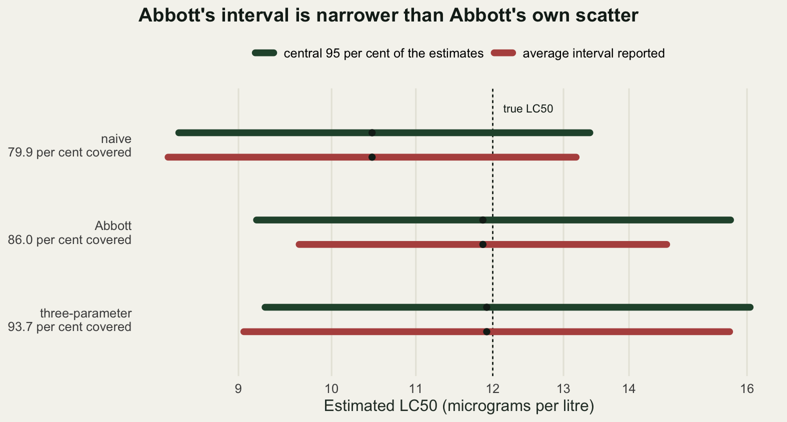
The naive fit is wrong, and wrong in a direction that matters. Background mortality lifts the observed proportion at every concentration, and it lifts it most where the toxicant is killing least, so the fitted curve slides towards lower concentrations. Over 1000 data sets the naive LC50 runs 12.4 per cent below the truth and its nominal 95 per cent interval covers the truth in 79.9 per cent of trials. Nothing in the output of that fit is a warning: it converges, its residuals look fine, and the standard error it reports, 0.118 on the log scale, matches the scatter of its own estimates, 0.117, almost exactly. The interval is the right width in the wrong place, which is the one failure that no diagnostic computed from the fit alone can see.
Abbott’s correction removes almost all of the bias. The corrected estimator sits 0.8 per cent below the truth on average, which is the calibration line this check needs. Its interval is another matter. Across the same 1000 data sets the spread of the Abbott estimates on the log scale is 0.142, while the average standard error it reports is 0.106: the reported interval is 0.747 of its honest width, and it covers the truth 86.0 per cent of the time rather than 95. The missing variance is the control group’s own, which the correction spends and never accounts for.
The three-parameter fit gets both parts right. It sits 0.1 per cent below the truth, its estimates have a spread of 0.143 on the log scale, which is no better than Abbott’s, and the average standard error it reports is 0.140, or 0.981 of the honest width, so coverage comes out at 93.7 per cent. Read those lines together and the result is sharper than it first looks. Abbott’s correction is not more precise than estimating the asymptote; the two estimators scatter by the same amount. Abbott’s is only more confident. The extra width of the three-parameter interval is not a cost of the method, it is the cost of not knowing the control mortality, and that cost was there all along.
One honest wrinkle in the three-parameter fit: in 12.2 per cent of these trials the control group shows no deaths at all, and in 12.0 per cent the estimated asymptote finishes on its lower bound. That is not a failure, it is what maximum likelihood does with a zero count, but it does mean the reported standard error for that parameter is not interpretable in those runs. Coverage for the LC50 holds up anyway.
Check 2: overdispersion from the test vessel
Animals are not exposed one at a time. They are exposed in vessels, and everything that varies between vessels while staying constant within them, oxygen, temperature, the actual concentration in that beaker, a batch of animals from the same brood, makes the animals in a vessel more alike than two animals picked from different vessels. The binomial likelihood has no room for this. It counts every animal as an independent trial, so it counts the experiment as bigger than it is.
The simulation puts 4 vessels of 20 animals at each of the same five concentrations, 400 animals in all, and gives each vessel a mortality probability drawn from a beta distribution centred on the true curve with an intraclass correlation of 0.10. Control mortality is switched off here so that only one thing is wrong at a time. Three analyses run on each data set: an ordinary binomial GLM on the vessel-level counts, the same fit with a quasi-binomial dispersion estimate and a t reference distribution, and a beta-binomial fit by maximum likelihood with the correlation as a third parameter. The theoretical design effect for this design, one plus the number of animals per vessel minus one times the correlation, is 2.9.
set.seed(20260801)
k_ves <- 4; m_ves <- 20; rho_true <- 0.10
xv <- rep(conc, each = k_ves)
n_ves <- length(xv); mv <- rep(m_ves, n_ves)
pv <- p_true(xv, b_true, e_true, 0)

nll_bb <- function(par, x, dead, m) {
  bb <- exp(par[1]); le <- par[2]; r <- plogis(par[3])
  p <- pmin(pmax(plogis(bb * (log(x) - le)), 1e-8), 1 - 1e-8)
  s <- (1 - r) / r
  -sum(lbeta(dead + p * s, m - dead + (1 - p) * s) - lbeta(p * s, (1 - p) * s))
}
fit_bb <- function(x, dead, m) {
  gg <- fit2(x, dead, m)
  st <- c(log(max(gg$co[2], 0.3)), -gg$co[1] / gg$co[2], qlogis(0.05))
  o <- optim(st, nll_bb, x = x, dead = dead, m = m, method = "L-BFGS-B",
             lower = c(-2, log(0.05), -10), upper = c(3, log(2000), 2),
             control = list(maxit = 1000, factr = 1e9))
  V <- solve(optimHess(o$par, nll_bb, x = x, dead = dead, m = m))
  c(lx = o$par[2], se = sqrt(V[2, 2]), rho = plogis(o$par[3]),
    conv = o$convergence)
}

n_rep2 <- 1000
sh <- (1 - rho_true) / rho_true
pmat <- matrix(rbeta(n_rep2 * n_ves, rep(pv * sh, each = n_rep2),
                     rep((1 - pv) * sh, each = n_rep2)), n_rep2, n_ves)
ymat <- matrix(rbinom(n_rep2 * n_ves, m_ves, pmat), n_rep2, n_ves)

res2 <- t(vapply(seq_len(n_rep2), function(i) {
  y <- ymat[i, ]
  gg <- fit2(xv, y, mv)
  b0 <- lc_of(gg$co, gg$V, 0.5)
  pr <- (y / m_ves - gg$mu) / sqrt(gg$mu * (1 - gg$mu) / m_ves)
  z <- fit_bb(xv, y, mv)
  c(b0, phi = sum(pr^2) / gg$df, unname(z))
}, numeric(7)))
colnames(res2) <- c("lx", "se", "phi", "bb_lx", "bb_se", "bb_rho", "conv")

tq <- qt(0.975, n_ves - 2)
print(round(c(replicates = n_rep2, vessels_per_level = k_ves,
              animals_per_vessel = m_ves, total_animals = n_ves * m_ves,
              rho = rho_true, design_effect_theory = 1 + (m_ves - 1) * rho_true,
              quasi_df = n_ves - 2,
              nonconvergence = sum(res2[, "conv"] != 0)), 3))
replicates vessels_per_level animals_per_vessel
1000.0 4.0 20.0
total_animals rho design_effect_theory
400.0 0.1 2.9
quasi_df nonconvergence
18.0 0.0 print(round(c(sd_log_binomial = sd(res2[, "lx"]),
mean_se_binomial = mean(res2[, "se"]),
design_effect_measured = (sd(res2[, "lx"]) / mean(res2[, "se"]))^2,
mean_dispersion = mean(res2[, "phi"]),
mean_rho_hat = mean(res2[, "bb_rho"]),
sd_log_betabin = sd(res2[, "bb_lx"]),
mean_se_betabin = mean(res2[, "bb_se"])), 4)) sd_log_binomial mean_se_binomial design_effect_measured
0.1052 0.0596 3.1135
mean_dispersion mean_rho_hat sd_log_betabin
2.8109 0.0862 0.1028
mean_se_betabin
0.0935 print(round(c(design_effect_measured = (sd(res2[, "lx"]) / mean(res2[, "se"]))^2,
mean_dispersion = mean(res2[, "phi"])), 3))design_effect_measured mean_dispersion
3.114 2.811 print(round(c(binomial = 100 * mean(abs(res2[, "lx"] - lt) < 1.96 * res2[, "se"]),
quasibinomial = 100 * mean(abs(res2[, "lx"] - lt) <
tq * res2[, "se"] * sqrt(res2[, "phi"])),
betabinomial = 100 * mean(abs(res2[, "bb_lx"] - lt) <
1.96 * res2[, "bb_se"])), 2)) binomial quasibinomial betabinomial
75.0 93.3 92.0 print(round(c(width_factor_quasi = mean(tq * res2[, "se"] * sqrt(res2[, "phi"])) /
mean(1.96 * res2[, "se"])), 2))width_factor_quasi
1.78 print(round(c(effective_animals = n_ves * m_ves /
((sd(res2[, "lx"]) / mean(res2[, "se"]))^2))))effective_animals
128 est <- data.frame(lc = res2[, "lx"])
se_bin <- mean(res2[, "se"])
se_qb <- mean(res2[, "se"] * sqrt(res2[, "phi"]))
gl <- seq(log(7.5), log(19), length.out = 400)
dens <- rbind(
data.frame(lc = gl, d = dnorm(gl, lt, se_bin), what = "binomial"),
data.frame(lc = gl, d = dnorm(gl, lt, se_qb), what = "quasi-binomial"))
dens$what <- factor(dens$what, levels = c("binomial", "quasi-binomial"))
brk <- c(8, 10, 12, 14, 16, 18)
ggplot(est, aes(lc)) +
geom_histogram(aes(y = after_stat(density)), bins = 45,
fill = te_pal$sage, colour = NA) +
geom_line(data = dens, aes(lc, d, colour = what), linewidth = 0.9) +
geom_vline(xintercept = lt, colour = te_pal$ink, linetype = "22",
linewidth = 0.5) +
annotate("text", x = lt + 0.06, y = 6.4, label = "true LC50", hjust = 0,
size = 3, colour = te_pal$ink) +
scale_x_continuous(breaks = log(brk), labels = as.character(brk)) +
coord_cartesian(xlim = log(c(7.5, 19))) +
scale_colour_manual(values = c(binomial = te_pal$clay,
"quasi-binomial" = te_pal$forest), name = NULL) +
labs(x = "Estimated LC50 (micrograms per litre)",
y = "Density on the log concentration scale",
title = "The binomial standard error describes a narrower experiment") +
theme_te() +
theme(legend.position = "top")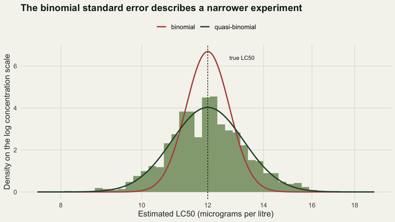
The estimates scatter with a standard deviation of 0.1052 on the log scale while the binomial fit reports an average standard error of 0.0596, so the measured design effect is 3.114 against a theoretical 2.9. The nominal 95 per cent interval covers the truth in 75.0 per cent of trials. Put the other way round: 400 animals arranged in 20 vessels carry the information of 128 animals tested one to a beaker, and an analysis that ignores the arrangement will report the interval that 400 independent animals would have earned.
Both repairs help and they do not help equally. The quasi-binomial scales the standard error by the square root of the estimated dispersion, which averages 2.811 here, and refers it to a t distribution on 18 degrees of freedom; that widens the interval by a factor of 1.78 and brings coverage to 93.3 per cent. The beta-binomial fit estimates the intraclass correlation directly and recovers 0.0862 against a true 0.1, and its coverage comes out at 92.0 per cent. Neither repair reaches 95, and the maximum likelihood fit with the correct likelihood is the one that falls furthest, which is not what most readers would predict. The reason is that its standard error is a curvature estimate at the maximum that treats the estimated correlation as known, exactly the mistake Abbott’s correction makes in check 1, and it refers the result to a normal quantile rather than a t. The quasi-binomial is cruder and its t reference happens to pay for the estimation of the dispersion.
None of this is visible in the estimate itself. The scatter of the beta-binomial estimates, 0.1028 on the log scale, is no better than the binomial one, and it is not supposed to be: overdispersion does not bias the LC50, it only inflates its variance. The whole defect lives in the second decimal place of a standard error, which is why the standard advice to plot the residuals is not enough here. If you want a diagnostic rather than a repair, the randomised quantile residuals in Checking a bounded-response model will show the extra spread on a scale where it can be read.
Check 3: extrapolating below the lowest tested dose
Regulatory numbers are not always LC50s. An assessment that wants a concentration with little effect asks for an LC10, an LC5 or an LC1, and those live in the lower tail of a curve that was fitted to data in the middle. The check measures two things: how far apart three standard curve shapes end up when they are read below the tested range, and how much a single extra treatment at a very low concentration buys.
Two designs share a total of 200 animals. The classic design puts 40 animals at each of five concentrations spaced by a factor of 1.45, with the lowest chosen so that its true mortality is 25.097 per cent, which is a design that satisfies every guideline for an LC50. The reallocated design drops the five tested levels to 30 animals each and opens a sixth level far below them, 50 animals at 2.5 micrograms per litre, where the true mortality is 3.074 per cent. The same three link functions are fitted to both: logit, which is the generating truth here, probit and complementary log-log.
To separate model shape from sampling noise the check does the arithmetic twice. The deterministic part fits the three shapes to the expected proportions with the sampling noise turned off, so any difference between the fitted curves is pure shape. The stochastic part repeats the whole exercise on 400 simulated data sets per design and records the spread across shapes and the width of each interval.
set.seed(20260801)
links <- c("logit", "probit", "cloglog")
lev <- c(0.50, 0.10, 0.05, 0.01)
ptr <- function(x) plogis(b_true * (log(x) - log(e_true)))
dA <- list(x = c(7.3, 10.6, 15.4, 22.3, 32.3), n = rep(40, 5))
dB <- list(x = c(2.5, 7.3, 10.6, 15.4, 22.3, 32.3), n = c(50, 30, 30, 30, 30, 30))
n_rep3 <- 400

true_lc <- exp(log(e_true) + qlogis(lev) / b_true)
print(round(c(total_animals_A = sum(dA$n), total_animals_B = sum(dB$n),
              per_level_A = dA$n[1], per_level_B = dB$n[2],
              lowest_group_B = dB$n[1],
              spacing_A = mean(dA$x[-1] / dA$x[-length(dA$x)]),
              lowest_A = min(dA$x), response_at_lowest_A_pct = 100 * ptr(min(dA$x)),
              lowest_B = min(dB$x), response_at_lowest_B_pct = 100 * ptr(min(dB$x)),
              expected_deaths_at_lowest_B = dB$n[1] * ptr(min(dB$x)),
              replicates = n_rep3), 3))
total_animals_A total_animals_B
200.000 200.000
per_level_A per_level_B
40.000 30.000
lowest_group_B spacing_A
50.000 1.450
lowest_A response_at_lowest_A_pct
7.300 25.097
lowest_B response_at_lowest_B_pct
2.500 3.074
expected_deaths_at_lowest_B replicates
1.537 400.000 print(round(setNames(true_lc, paste0("true_LC", 100 * lev)), 3))true_LC50 true_LC10 true_LC5 true_LC1
12.000 4.420 3.147 1.486 det_lc <- function(d) sapply(links, function(lk) {
f <- fit2(d$x, round(ptr(d$x) * 1e6), rep(1e6, length(d$x)), lk)
sapply(lev, function(p) exp(lc_of(f$co, f$V, p, lk)["lx"]))
})
dlA <- det_lc(dA); dlB <- det_lc(dB)
rownames(dlA) <- rownames(dlB) <- paste0("LC", 100 * lev)
print(round(dlA, 3)) logit probit cloglog
LC50 12.000 12.041 12.508
LC10 4.420 4.560 3.097
LC5 3.147 3.463 1.816
LC1 1.486 2.067 0.543print(round(dlB, 3)) logit probit cloglog
LC50 12.000 11.903 12.937
LC10 4.420 4.347 3.546
LC5 3.147 3.267 2.163
LC1 1.486 1.912 0.706print(round(rbind(design_A = apply(dlA, 1, function(z) max(z) / min(z)),
design_B = apply(dlB, 1, function(z) max(z) / min(z))), 3)) LC50 LC10 LC5 LC1
design_A 1.042 1.473 1.907 3.807
design_B 1.087 1.246 1.511 2.709sim_design <- function(d) {
y <- matrix(rbinom(n_rep3 * length(d$x), rep(d$n, each = n_rep3),
rep(ptr(d$x), each = n_rep3)), n_rep3, length(d$x))
out <- vapply(seq_len(n_rep3), function(i) {
z <- vapply(links, function(lk) {
f <- fit2(d$x, y[i, ], d$n, lk)
as.vector(vapply(lev, function(p) lc_of(f$co, f$V, p, lk), numeric(2)))
}, numeric(2 * length(lev)))
c(spread = apply(matrix(z[seq(1, 2 * length(lev), 2), ], length(lev)), 1,
function(v) exp(max(v) - min(v))),
fold = exp(2 * 1.96 * z[seq(2, 2 * length(lev), 2), 1]))
}, numeric(2 * length(lev)))
round(rbind(shape_spread = rowMeans(out[seq_along(lev), ]),
fold_width_logit = rowMeans(out[length(lev) + seq_along(lev), ])), 3)
}
sA <- sim_design(dA); sB <- sim_design(dB)
colnames(sA) <- colnames(sB) <- paste0("LC", 100 * lev)
print(sA) LC50 LC10 LC5 LC1
shape_spread 1.042 1.478 1.923 3.933
fold_width_logit 1.365 2.266 2.836 4.814print(sB) LC50 LC10 LC5 LC1
shape_spread 1.102 1.193 1.413 2.437
fold_width_logit 1.391 1.959 2.328 3.490print(round(c(width_gain_LC5 = sA["fold_width_logit", "LC5"] /
sB["fold_width_logit", "LC5"],
width_cost_LC50 = sB["fold_width_logit", "LC50"] /
sA["fold_width_logit", "LC50"],
spread_gain_LC5 = sA["shape_spread", "LC5"] /
sB["shape_spread", "LC5"]), 3)) width_gain_LC5 width_cost_LC50 spread_gain_LC5
1.218 1.019 1.361 one_set <- function(d) {
y <- rbinom(length(d$x), d$n, ptr(d$x))
cur <- do.call(rbind, lapply(links, function(lk) {
f <- fit2(d$x, y, d$n, lk)
gx <- exp(seq(log(1.2), log(40), length.out = 250))
eta <- f$co[1] + f$co[2] * log(gx)
mu <- switch(lk, logit = plogis(eta), probit = pnorm(eta),
cloglog = 1 - exp(-exp(eta)))
data.frame(x = gx, y = mu, link = lk)
}))
list(cur = cur, obs = data.frame(x = d$x, y = pmax(y / d$n, 0.0012)))
}
set.seed(20260801)
oA <- one_set(dA); oB <- one_set(dB)
lab <- c("classic design", "with a low-dose group")
cur3 <- rbind(cbind(oA$cur, panel = lab[1]), cbind(oB$cur, panel = lab[2]))
obs3 <- rbind(cbind(oA$obs, panel = lab[1]), cbind(oB$obs, panel = lab[2]))
cur3$panel <- factor(cur3$panel, levels = lab)
obs3$panel <- factor(obs3$panel, levels = lab)
vl <- data.frame(panel = factor(lab, levels = lab), x = c(min(dA$x), min(dB$x)))
cur3$link <- factor(cur3$link, levels = links)
ggplot(cur3, aes(x, y, colour = link)) +
geom_hline(yintercept = c(0.10, 0.05, 0.01), colour = "#b8b6a4",
linewidth = 0.6) +
geom_vline(data = vl, aes(xintercept = x), colour = te_pal$ink,
linetype = "22", linewidth = 0.5) +
geom_text(data = vl, aes(x = x * 1.08, y = 0.0016), inherit.aes = FALSE,
label = "lowest tested dose", hjust = 0, size = 3,
colour = te_pal$ink) +
geom_line(linewidth = 0.9) +
geom_point(data = obs3, aes(x, y), inherit.aes = FALSE, colour = te_pal$ink,
size = 2.2) +
facet_wrap(~panel) +
scale_x_log10(breaks = c(1.5, 3, 6, 12, 25),
labels = c("1.5", "3", "6", "12", "25")) +
scale_y_log10(breaks = c(0.001, 0.01, 0.05, 0.1, 0.3, 1),
labels = c("0.001", "0.01", "0.05", "0.10", "0.30", "1.00")) +
coord_cartesian(ylim = c(0.001, 1)) +
scale_colour_manual(values = c(logit = te_pal$forest, probit = te_pal$gold,
cloglog = te_pal$clay), name = NULL) +
labs(x = "Concentration (micrograms per litre)", y = "Proportion dead",
title = "The shapes agree where the data are and part company below") +
theme_te() +
theme(legend.position = "top",
strip.text = element_text(colour = te_pal$ink, face = "bold"))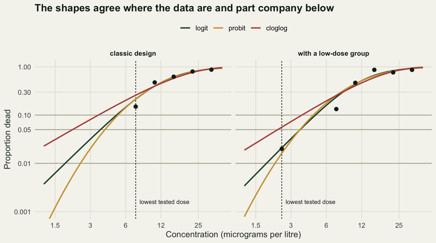
With sampling noise switched off, the three shapes fitted to the classic design return LC50s of 12.000, 12.041 and 12.508, a spread of 1.042. At the LC5 they return 3.147, 3.463 and 1.816, a spread of 1.907, and at the LC1 the spread is 3.807. This is not estimation error. It is what three curve families that agree on the same middle do when they are asked about a region where no animal was tested, and no amount of data at the tested concentrations reduces it, because the deterministic calculation already assumes an infinite sample.
The simulated runs put numbers on the cost. Averaged over 400 data sets from the classic design, the three shapes differ by a factor of 1.923 at the LC5 and 3.933 at the LC1, while the logit fit’s own 95 per cent interval spans a factor of 2.836 at the LC5 and 4.814 at the LC1. Two things follow. The disagreement between the shapes at the LC5 is most of the width of the interval that gets reported, so an assessment that fits one shape and quotes its interval is understating the uncertainty by an amount no residual plot can reveal. And the interval at the LC1 covers a factor of 4.814 from end to end, which is a way of saying that the experiment did not measure it.
Taking 10 animals from each tested level and putting 50 into a sixth group at 2.5 micrograms per litre, where the expected number of deaths is 1.537, does more than it looks like it should. The shape spread at the LC5 falls from 1.923 to 1.413, and the logit interval at the LC5 narrows from a factor of 2.836 to 2.328, a gain of 1.218. The price is paid at the LC50, whose interval widens by a factor of 1.019. A group in which almost nothing happens is not an uninformative group: an observed zero or one death out of 50 at a concentration where the cloglog shape expects several is evidence against the cloglog shape. What it cannot do is close the gap. Even with the extra group the three shapes still differ by a factor of 2.437 at the LC1, so the honest report of an LC1 from any design like this is a range with a curve family attached to it.
Check 4: nominal concentration is not exposure
The concentration on the axis is usually the nominal one: what was weighed out and diluted. What the animals experienced can be lower, because the compound sorbs to glass and to the animals, volatilises, degrades in light, or is taken up. And it varies from vessel to vessel, because none of those processes is identical in two beakers.
Model this as a systematic loss plus multiplicative scatter: the actual concentration in a vessel is the nominal concentration at a recovery of 70 per cent, times a lognormal factor with median one, so that half the vessels sit above the nominal recovery and half below. The design has 4 vessels of 15 animals at each of five nominal levels, and the check fits the same curve three ways: on nominal concentration, on the actual concentration in each vessel, and on a measured concentration, which is the actual one seen through an analytical error with a log standard deviation of 0.15. The scatter is swept from zero to 0.8 and each point on the sweep uses 400 data sets. Estimates are summarised by their geometric mean, which is the natural average on a log concentration axis.
set.seed(20260801)
f_loss <- 0.70; s_an <- 0.15; k_ex <- 4; m_ex <- 15
nom <- conc / f_loss
xn <- rep(nom, each = k_ex); nx <- length(xn); mx <- rep(m_ex, nx)
lt10 <- log(e_true) + qlogis(0.1) / b_true
n_rep4 <- 400
s_grid <- c(0, 0.15, 0.30, 0.45, 0.60, 0.80)
print(round(c(nominal = nom), 2))
nominal1 nominal2 nominal3 nominal4 nominal5
5.29 9.57 17.14 30.86 55.57 print(round(c(vessels_per_level = k_ex, animals_per_vessel = m_ex,
total_animals = nx * m_ex, recovery_pct = 100 * f_loss,
analytical_sd = s_an, replicates = n_rep4,
true_nominal_lc50 = e_true / f_loss,
true_nominal_lc10 = exp(lt10) / f_loss), 3)) vessels_per_level animals_per_vessel total_animals recovery_pct
4.000 15.000 300.000 70.000
analytical_sd replicates true_nominal_lc50 true_nominal_lc10
0.150 400.000 17.143 6.314 sweep <- t(vapply(s_grid, function(s) {
del <- matrix(rnorm(n_rep4 * nx, 0, s), n_rep4, nx)
act <- exp(log(rep(xn, each = n_rep4) * f_loss) + del)
y <- matrix(rbinom(n_rep4 * nx, m_ex,
plogis(b_true * (log(act) - log(e_true)))), n_rep4, nx)
meas <- act * exp(matrix(rnorm(n_rep4 * nx, 0, s_an), n_rep4, nx))
z <- t(vapply(seq_len(n_rep4), function(i) {
cn <- fit2(xn, y[i, ], mx)$co; ca <- fit2(act[i, ], y[i, ], mx)$co
cm <- fit2(meas[i, ], y[i, ], mx)$co
c(cn[2], -cn[1] / cn[2], (qlogis(0.1) - cn[1]) / cn[2],
ca[2], -ca[1] / ca[2], (qlogis(0.1) - ca[1]) / ca[2],
cm[2], -cm[1] / cm[2], (qlogis(0.1) - cm[1]) / cm[2])
}, numeric(9)))
c(exposure_sd = s,
slope_nominal = mean(z[, 1]) / b_true,
lc50_nominal = exp(mean(z[, 2]) - log(e_true / f_loss)),
lc10_nominal = exp(mean(z[, 3]) - (lt10 - log(f_loss))),
slope_actual = mean(z[, 4]) / b_true,
lc50_actual = exp(mean(z[, 5]) - log(e_true)),
lc10_actual = exp(mean(z[, 6]) - lt10),
slope_measured = mean(z[, 7]) / b_true,
lc50_measured = exp(mean(z[, 8]) - log(e_true)),
lc10_measured = exp(mean(z[, 9]) - lt10))
}, numeric(10)))
print(round(sweep, 4)) exposure_sd slope_nominal lc50_nominal lc10_nominal slope_actual
[1,] 0.00 1.0193 1.0022 1.0085 1.0193
[2,] 0.15 0.9868 1.0031 0.9765 1.0092
[3,] 0.30 0.9453 1.0090 0.9302 1.0115
[4,] 0.45 0.8695 1.0037 0.8325 1.0137
[5,] 0.60 0.7908 0.9933 0.7084 1.0201
[6,] 0.80 0.7153 1.0024 0.5787 1.0111
lc50_actual lc10_actual slope_measured lc50_measured lc10_measured
[1,] 1.0022 1.0085 0.9909 1.0027 0.9780
[2,] 1.0003 0.9984 0.9818 1.0001 0.9675
[3,] 1.0077 1.0058 0.9847 1.0064 0.9751
[4,] 0.9974 0.9982 0.9830 0.9967 0.9655
[5,] 0.9924 0.9976 0.9892 0.9910 0.9632
[6,] 1.0100 1.0068 0.9877 1.0068 0.9781print(round(sweep[4, -1], 3)) slope_nominal lc50_nominal lc10_nominal slope_actual lc50_actual
0.869 1.004 0.832 1.014 0.997
lc10_actual slope_measured lc50_measured lc10_measured
0.998 0.983 0.997 0.965 print(round(c(quartile_low = exp(qnorm(0.25) * 0.45),
quartile_high = exp(qnorm(0.75) * 0.45)), 3)) quartile_low quartile_high
0.738 1.355 print(round(c(attenuation_at_045 = 100 * (1 - sweep[4, "slope_nominal"] /
sweep[1, "slope_nominal"]),
lc10_shortfall_pct = 100 * (1 - sweep[4, "lc10_nominal"]),
lc50_shift_pct = 100 * (sweep[4, "lc50_nominal"] - 1)), 1))attenuation_at_045.slope_nominal lc10_shortfall_pct.lc10_nominal
14.7 16.8
lc50_shift_pct.lc50_nominal
0.4 swl <- data.frame(
s = rep(sweep[, "exposure_sd"], 3),
ratio = c(sweep[, "slope_nominal"], sweep[, "lc50_nominal"],
sweep[, "lc10_nominal"]),
what = rep(c("slope", "LC50", "LC10"), each = nrow(sweep)))
swl$what <- factor(swl$what, levels = c("LC50", "slope", "LC10"))
ggplot(swl, aes(s, ratio, colour = what)) +
geom_hline(yintercept = 1, colour = "#b8b6a4", linewidth = 0.8) +
geom_vline(xintercept = 0.45, colour = te_pal$ink, linetype = "22",
linewidth = 0.5) +
annotate("text", x = 0.465, y = 1.075, label = "the scatter quoted in the text",
hjust = 0, size = 3, colour = te_pal$ink) +
geom_line(linewidth = 0.9) +
geom_point(size = 2.4) +
scale_colour_manual(values = c(LC50 = te_pal$forest, slope = te_pal$gold,
LC10 = te_pal$clay), name = NULL) +
scale_y_continuous(limits = c(0.55, 1.1)) +
labs(x = "Log standard deviation of actual exposure between vessels",
y = "Estimate divided by truth",
title = "The LC50 survives what the LC10 does not") +
theme_te() +
theme(legend.position = "top")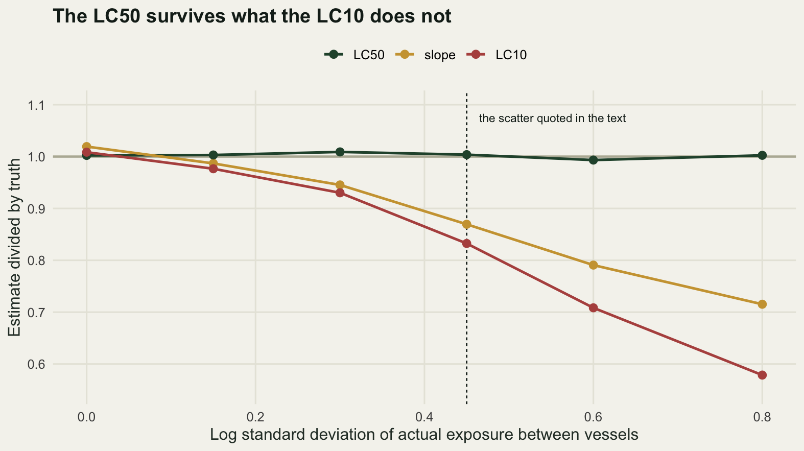
The systematic part is the easy part. A recovery of 70 per cent moves the whole curve: the nominal concentration that kills half the animals is 17.143 when the actual LC50 is 12, and dividing by the recovery puts it back. Any laboratory that measures its concentrations can do this arithmetic, and the check scores the fits against the correct nominal target so that the systematic shift does not contaminate the rest.
The scatter is the part that hides. At a log standard deviation of 0.45, which puts the middle half of the vessels between 0.738 and 1.355 times the median exposure, the slope estimated on the nominal axis is 14.7 per cent below what the same fit returns with no scatter at all, and the LC10 comes out 16.8 per cent below its true nominal value of 6.314. The LC50 moves by 0.4 per cent. The curve flattens around a fixed point, and the fixed point is the LC50.
That is a measurement error problem with a wrinkle that is worth naming. In the classical version, described in Measurement error and regression dilution, the recorded predictor is a noisy version of the true one and the slope is pulled towards zero by the ratio of signal to total variance. Here the recorded predictor is the nominal concentration, which is fixed by the experimenter, and the true exposure scatters around it. That is Berkson error, and in a linear model it would leave the slope alone. It flattens this curve anyway, because the fitted curve is the average of logistic curves centred at different places, and an average of sigmoids is a shallower sigmoid. The mechanism is not regression dilution and the consequence looks identical.
Fitting on the vessel-specific actual concentrations removes the flattening entirely: the slope ratio returns to 1.014 at the same scatter, and the LC10 to 0.998. Fitting on measured concentrations with an analytical log standard deviation of 0.15 recovers most of it, a slope ratio of 0.983 and an LC10 ratio of 0.965, with the residual gap now being genuine classical error in the analytical measurement. Measuring the vessels is worth more than any of the modelling in this post.
There is one direction of the result that deserves stating plainly, because it is the opposite of a comforting story. The number that survives the defect is the LC50, which is the number that is easiest to check against other laboratories. The number that fails is the LC10, which is the number an assessment uses when it wants a concentration that does little harm, and it fails in the direction that makes the compound look more toxic than it is. That is conservative, and it is still wrong, and it will not be conservative for a compound whose exposure scatter runs the other way.
Check 5: which null the combination is tested against
Everything above stays inside one assay with one toxicant. Add a second stressor, a warming treatment or a second compound crossed with the first, and the report stops being a curve and becomes a verdict: the combination is synergistic, or antagonistic, or neither. That verdict is not read off the counts. It is read off a null, and two nulls are in common use that disagree with each other about what acting independently means.
Both of them start from the corrected mortalities of check 1. Take the control mortality out of every treated cell the way Abbott does, so that each cell holds a mortality among the animals the control conditions would have spared. Independent action, the multiplicative null, says the survivors of one stressor meet the other on the same terms as anybody else, so the corrected survival under both is the product of the two corrected survivals. Response addition, the additive null, says the killed fractions add, so the corrected mortality under both is the sum of the two corrected mortalities. The sum is the larger of the two by exactly the product of the two corrected mortalities, so response addition always expects more death than independent action does, and any joint count that lands in the gap between them is called synergistic by one null and antagonistic by the other.
The check runs that arithmetic on a 2 x 2 table with a bootstrap attached, then asks the second question: what the multiplicative null implies for the interaction term of a logistic model, which is a third answer again, and the one the software hands you without being asked.
set.seed(20260801)
tw_n <- 200
tw_dead <- c(control = 16, stressor_A = 99, stressor_B = 99, both = 163)
tw_c <- tw_dead[["control"]] / tw_n
tw_abb <- (tw_dead / tw_n - tw_c) / (1 - tw_c)
undo <- function(m) tw_n * (tw_c + (1 - tw_c) * m)
print(rbind(dead = tw_dead, alive = tw_n - tw_dead))
control stressor_A stressor_B both
dead 16 99 99 163
alive 184 101 101 37print(round(c(animals_per_cell = tw_n, control_mortality = tw_c,
corrected_A = tw_abb[["stressor_A"]], corrected_B = tw_abb[["stressor_B"]],
corrected_both = tw_abb[["both"]],
sum_of_the_two = tw_abb[["stressor_A"]] + tw_abb[["stressor_B"]]), 4)) animals_per_cell control_mortality corrected_A corrected_B
200.0000 0.0800 0.4511 0.4511
corrected_both sum_of_the_two
0.7989 0.9022 tw_res <- c(observed = tw_dead[["both"]],
multiplicative = undo(1 - (1 - tw_abb[["stressor_A"]]) *
(1 - tw_abb[["stressor_B"]])),
additive = undo(tw_abb[["stressor_A"]] + tw_abb[["stressor_B"]]))
tw_res <- c(tw_res, excess = tw_res[["observed"]] - tw_res[["multiplicative"]],
deficit = tw_res[["additive"]] - tw_res[["observed"]],
window = tw_res[["additive"]] - tw_res[["multiplicative"]])
print(round(tw_res, 2)) observed multiplicative additive excess deficit
163.00 144.56 182.00 18.44 19.00
window
37.44 n_boot <- 4000
bt <- matrix(rbinom(4 * n_boot, tw_n, rep(tw_dead / tw_n, each = n_boot)), n_boot, 4)
bc <- bt[, 1] / tw_n
ba <- (bt / tw_n - bc) / (1 - bc)
bx <- function(m) tw_n * (bc + (1 - bc) * m)
b_mult <- bt[, 4] - bx(1 - (1 - ba[, 2]) * (1 - ba[, 3]))
b_add <- bx(ba[, 2] + ba[, 3]) - bt[, 4]
tw_ci <- c(bootstrap_replicates = n_boot,
excess_lo = unname(quantile(b_mult, 0.025)),
excess_hi = unname(quantile(b_mult, 0.975)),
deficit_lo = unname(quantile(b_add, 0.025)),
deficit_hi = unname(quantile(b_add, 0.975)),
additive_over_all_animals_pct = 100 * mean(bx(ba[, 2] + ba[, 3]) > tw_n))
print(round(tw_ci, 2)) bootstrap_replicates excess_lo
4000.00 3.53
excess_hi deficit_lo
34.25 -5.00
deficit_hi additive_over_all_animals_pct
42.00 4.23 Each stressor on its own kills 45.1 per cent of the animals the control conditions would have spared, and together they leave 163 of 200 dead. Independent action expects 144.6 deaths and response addition expects 182, so one and the same table sits 18.4 deaths above what one null allows and 19 deaths below what the other one predicts. The verdicts are synergy and antagonism, on one table, before any test has been run. The gap between the two expectations is 37.4 animals wide, and every joint count inside it gets both labels.
A parametric bootstrap over all four cells, which prices the noise in the single-stressor cells instead of treating them as known, keeps the synergy verdict clear of zero at 3.5 to 34.3 deaths, and does not do the same for the antagonism verdict, whose interval runs from -5 to 42. The two labels are not equally well supported here even though they come from the same counts. The additive null is also straining: the two corrected mortalities sum to 0.9022, and in 4.23 per cent of the bootstrap replicates they sum past one, where response addition expects more deaths than there are animals.
set.seed(20260801)
imp_int <- function(a, sc) qlogis(a^2 * sc) - 2 * qlogis(a * sc) + qlogis(sc)
fA <- c(0, 1, 0, 1); fB <- c(0, 0, 1, 1)
a_ver <- 0.55; s_ver <- 0.92
p_ver <- c(s_ver, a_ver * s_ver, a_ver * s_ver, a_ver^2 * s_ver)
g_surv <- glm(p_ver ~ fA * fB, family = binomial, weights = rep(1e6, 4))
g_dead <- glm(1 - p_ver ~ fA * fB, family = binomial, weights = rep(1e6, 4))
print(round(c(kill_fraction = 1 - a_ver, control_survival = s_ver,
              closed_form = imp_int(a_ver, s_ver),
              glm_on_survival = unname(coef(g_surv)[4]),
              glm_on_deaths = unname(coef(g_dead)[4])), 6))
kill_fraction control_survival closed_form glm_on_survival
0.450000 0.920000 1.441435 1.441435
glm_on_deaths
-1.441435 lor22 <- function(alive, nn) {
aa <- alive + 0.5; dd <- nn - alive + 0.5
est <- log(aa[, 1]) + log(aa[, 4]) - log(aa[, 2]) - log(aa[, 3]) -
log(dd[, 1]) - log(dd[, 4]) + log(dd[, 2]) + log(dd[, 3])
cbind(est = est, se = sqrt(rowSums(1 / aa) + rowSums(1 / dd)))
}
n_rep6 <- 2000
kill6 <- seq(0.1, 0.8, by = 0.1)
ctl6 <- c(0.02, 0.08, 0.15)
sw6 <- do.call(rbind, lapply(ctl6, function(cm) {
sc <- 1 - cm
t(vapply(kill6, function(k) {
pk <- c(sc, (1 - k) * sc, (1 - k) * sc, (1 - k)^2 * sc)
mm <- matrix(rbinom(4 * n_rep6, tw_n, rep(pk, each = n_rep6)), n_rep6, 4)
zz <- lor22(mm, tw_n)
c(control_pct = 100 * cm, kill_pct = 100 * k, implied = imp_int(1 - k, sc),
simulated = mean(zz[, "est"]),
reject_pct = 100 * mean(abs(zz[, "est"] / zz[, "se"]) > 1.96),
gap_in_animals = k * k * sc * tw_n)
}, numeric(6)))
}))
print(round(sw6, 3)) control_pct kill_pct implied simulated reject_pct gap_in_animals
[1,] 2 10 1.217 1.217 46.85 1.96
[2,] 2 20 1.834 1.835 96.05 7.84
[3,] 2 30 2.250 2.273 99.95 17.64
[4,] 2 40 2.574 2.577 100.00 31.36
[5,] 2 50 2.846 2.842 100.00 49.00
[6,] 2 60 3.087 3.078 100.00 70.56
[7,] 2 70 3.308 3.342 100.00 96.04
[8,] 2 80 3.516 3.519 99.55 125.44
[9,] 8 10 0.372 0.394 14.30 1.84
[10,] 8 20 0.751 0.755 51.65 7.36
[11,] 8 30 1.059 1.057 83.95 16.56
[12,] 8 40 1.322 1.324 96.95 29.44
[13,] 8 50 1.555 1.558 99.55 46.00
[14,] 8 60 1.767 1.782 99.90 66.24
[15,] 8 70 1.966 1.961 99.35 90.16
[16,] 8 80 2.157 2.169 96.20 117.76
[17,] 15 10 0.167 0.169 8.10 1.70
[18,] 15 20 0.404 0.405 23.30 6.80
[19,] 15 30 0.628 0.631 50.50 15.30
[20,] 15 40 0.836 0.826 72.65 27.20
[21,] 15 50 1.029 1.036 88.30 42.50
[22,] 15 60 1.212 1.203 92.95 61.20
[23,] 15 70 1.388 1.381 91.10 83.30
[24,] 15 80 1.559 1.550 82.45 108.80print(c(replicates_per_point = n_rep6, animals_per_cell = tw_n))replicates_per_point animals_per_cell
2000 200 key5 <- c(largest_gap_to_simulation = max(abs(sw6[, "implied"] - sw6[, "simulated"])),
implied_at_10 = unname(sw6[9, "implied"]),
gap_at_10 = unname(sw6[9, "gap_in_animals"]),
reject_at_10 = unname(sw6[9, "reject_pct"]),
implied_at_60 = unname(sw6[14, "implied"]),
gap_at_60 = unname(sw6[14, "gap_in_animals"]),
reject_at_60 = unname(sw6[14, "reject_pct"]),
implied_clean_control = unname(sw6[1, "implied"]),
reject_clean_control = unname(sw6[1, "reject_pct"]))
print(round(key5, 3))largest_gap_to_simulation implied_at_10 gap_at_10
0.033 0.372 1.840
reject_at_10 implied_at_60 gap_at_60
14.300 1.767 66.240
reject_at_60 implied_clean_control reject_clean_control
99.900 1.217 46.850 pan <- c("implied interaction (log odds units)",
"share of tests reporting an interaction (per cent)")
sw6d <- as.data.frame(sw6)
sw6d$control <- factor(paste0(sw6d$control_pct, " per cent control mortality"),
levels = paste0(c(2, 8, 15), " per cent control mortality"))
long6 <- rbind(data.frame(kill = sw6d$kill_pct, y = sw6d$implied,
control = sw6d$control, panel = pan[1]),
data.frame(kill = sw6d$kill_pct, y = sw6d$reject_pct,
control = sw6d$control, panel = pan[2]))
long6$panel <- factor(long6$panel, levels = pan)
hl <- data.frame(panel = factor(pan, levels = pan), y = c(0, 5))
tl <- data.frame(panel = factor(pan[2], levels = pan), kill = 42, y = 11,
lab = "5 per cent, the nominal rate")
ggplot(long6, aes(kill, y, colour = control)) +
geom_hline(data = hl, aes(yintercept = y), colour = "#b8b6a4", linewidth = 0.8) +
geom_text(data = tl, aes(kill, y, label = lab), inherit.aes = FALSE, hjust = 0,
size = 3, colour = te_pal$ink) +
geom_line(linewidth = 0.9) +
geom_point(size = 2.2) +
facet_wrap(~panel, scales = "free_y") +
expand_limits(y = 0) +
scale_x_continuous(breaks = seq(10, 80, by = 10)) +
scale_colour_manual(values = c(te_pal$forest, te_pal$gold, te_pal$clay),
name = NULL) +
labs(x = "Percentage of the survivors each stressor kills on its own", y = NULL,
title = "Independent action leaves a term in the interaction slot") +
theme_te() +
theme(legend.position = "top",
strip.text = element_text(colour = te_pal$ink, face = "bold"))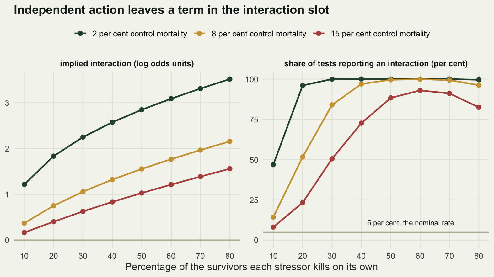
On the log odds scale the multiplicative null is not the absence of an interaction. If each stressor leaves a fraction a of the corrected survivors alive and the control survival is s0, the saturated logistic model fitted to survival carries an interaction term of exactly qlogis(a^2 * s0) - 2 * qlogis(a * s0) + qlogis(s0). At a kill of 45 per cent and a control survival of 0.92 that comes to 1.441, and a fit to the exact expected proportions returns the same value to six decimals, while the same fit on deaths returns it with the sign reversed. The sign is the part to carry away: counts generated by exact independent action arrive at a logistic model of mortality looking antagonistic. The sweep that follows reads that term off each simulated two by two table as the 0.5-corrected log odds ratio with the Woolf standard error rather than by refitting a model, a correction that keeps the estimate finite when a cell empties. Over the whole sweep the mean of 2000 simulated estimates never departs from the closed form by more than 0.033 log odds, which is what makes the formula usable as a check rather than a curiosity.
The size of that term is not a constant, and quoting one number for it is the mistake this check exists to prevent. It goes to zero as the stressors stop killing, it grows as they kill harder, and it depends on the control as much as on the treatments. With a control mortality of 8 per cent and each stressor killing a tenth of the corrected survivors, the implied interaction is 0.372 log odds, the two nulls differ by 1.84 animals in 200, which is well inside the sampling noise of a single cell, and the nominal 5 per cent test reports an interaction in 14.3 per cent of trials. At kills of 60 per cent the same three numbers are 1.767 log odds, 66.24 animals and 99.9 per cent. Clean the control up to 2 per cent and the tenth-kill case moves to 1.217 log odds and 46.9 per cent, because the logit scale stretches hardest where mortality is near zero. The reading that survives all of this is on the count scale: where both stressors kill hard the two nulls stand far apart and the label is chosen by the null rather than by the data, and where they kill lightly they agree to within a couple of animals and no test on a design of this size can separate them.
Report the observed joint count with both expectations printed beside it, and name the null in the sentence that carries the verdict, because a combination called synergistic without the null it is synergistic against is a number with no units on it. The general form of the point, that a null of no effect is a choice of scale rather than a property of the counts, is in Comparing significance is not a test; what this check adds is the arithmetic you can run on your own table before the label is written down.
The honest limit
Every check above knows the answer. On real data none of them tells you which defect you have, and the reason is that three of the first four leave the same fingerprint. Take the exposure scatter from check 4, with no beta-binomial mixture anywhere in the generating model, and run check 2’s diagnostics on it.
set.seed(20260801)
n_rep5 <- 300
del <- matrix(rnorm(n_rep5 * nx, 0, 0.45), n_rep5, nx)
act <- exp(log(rep(xn, each = n_rep5) * f_loss) + del)
y5 <- matrix(rbinom(n_rep5 * nx, m_ex,
                    plogis(b_true * (log(act) - log(e_true)))), n_rep5, nx)
res5 <- t(vapply(seq_len(n_rep5), function(i) {
  gg <- fit2(xn, y5[i, ], mx)
  pr <- (y5[i, ] / m_ex - gg$mu) / sqrt(gg$mu * (1 - gg$mu) / m_ex)
  z <- fit_bb(xn, y5[i, ], mx)
  c(phi = sum(pr^2) / gg$df, rho = unname(z["rho"]), conv = unname(z["conv"]))
}, numeric(3)))
print(round(c(replicates = n_rep5, exposure_sd = 0.45,
              mean_dispersion = mean(res5[, "phi"]),
              mean_rho_hat = mean(res5[, "rho"]),
              implied_design_effect = 1 + (m_ex - 1) * mean(res5[, "rho"]),
              nonconvergence = sum(res5[, "conv"] != 0)), 3))
replicates exposure_sd mean_dispersion
300.000 0.450 2.713
mean_rho_hat implied_design_effect nonconvergence
0.111 2.552 0.000 Exposure scatter of the size used in check 4 produces a dispersion statistic of 2.713 and an estimated intraclass correlation of 0.111, which implies a design effect of 2.552 for its 15 animals per vessel. Check 2’s own data, generated by a genuine beta-binomial mixture, gave a dispersion of 2.811. The two mechanisms are not distinguishable from the dispersion statistic, and that matters because the repairs are different. If the extra variance is heterogeneity in susceptibility between vessels, the quasi-binomial interval is the right answer and the point estimate was never biased. If it is exposure scatter, the interval is still too narrow and the slope is attenuated as well, so widening the interval treats the symptom and leaves the LC10 wrong.
The same ambiguity runs through the rest. Control mortality and a flattened curve both push the low-dose end of the fit upwards. A shape that is wrong in the tail and a genuine change in mechanism at low concentrations look identical in the tested range, which is where check 3 stops being about statistics. And all four of those checks assume the response is a smooth monotone function of concentration, which is the assumption that Hormesis and non-monotonic responses declines to make. The only check among those four that a laboratory can act on without a simulation is the one that involves no statistics at all: measure the concentrations in the vessels, report them, and fit on them.
Where to go next
Three of the first four defects are design problems wearing an analysis costume. The control group carries information about the lower asymptote and should be in the likelihood rather than in a correction factor. The vessel is the experimental unit and either belongs in the model or belongs in the standard error. The lowest tested concentration sets the floor under which every effective dose is an extrapolation, and one cheap group below it buys a measurable amount of tail. Only the exposure question needs a chemist rather than a statistician. The fifth defect is not a design problem at all: no allocation of animals fixes it, because the null is chosen in the sentence that reports the result.
For the interval machinery itself, Confidence intervals for effective doses compares the delta method used throughout this post with Fieller’s theorem and with profile likelihood, and shows how far the delta method drifts in the tail where check 3 works. For the diagnostic side, Checking a bounded-response model covers residuals for proportion data, which is the tool that finds the overdispersion in check 2 before it has cost you an interval.
References
Ritz C 2010 Environmental Toxicology and Chemistry 29(1):220-229 (10.1002/etc.7)
Ritz C, Baty F, Streibig JC, Gerhard D 2015 PLOS ONE 10(12):e0146021 (10.1371/journal.pone.0146021)
Williams DA 1975 Biometrics 31(4):949-952 (10.2307/2529820)
Abbott WS 1925 Journal of Economic Entomology 18(2):265-267 (10.1093/jee/18.2.265a)
Carroll RJ, Ruppert D, Stefanski LA, Crainiceanu CM 2006 Measurement Error in Nonlinear Models: A Modern Perspective. 2nd edition. Chapman and Hall/CRC, ISBN 978-1-58488-633-4