library(ggplot2)

te_pal <- list(forest = "#275139", green = "#2f8f63", sage = "#93a87f",
               clay = "#b5534e", gold = "#cda23f", line = "#dad9ca",
               ink = "#16241d", paper = "#f5f4ee")

theme_te <- function() {
  theme_minimal(base_size = 12) +
    theme(panel.grid.minor = element_blank(),
          panel.grid.major = element_line(colour = "#e7e6dc"),
          plot.background = element_rect(fill = "#f5f4ee", colour = NA),
          panel.background = element_rect(fill = "#f5f4ee", colour = NA),
          plot.title = element_text(face = "bold", colour = te_pal$ink),
          axis.title = element_text(colour = "#2c3a31"),
          axis.text = element_text(colour = "#2c3a31"))
}Comparing significance is not a test
R
interactions
hypothesis testing
statistical power
ecology tutorial
Significant at one site and not at the other is not evidence that the sites differ. Measuring the fallacy rate in R, and the interaction test that replaces it.
An open-top chamber experiment, run for three seasons at two sites on the same mountain: one at six hundred metres in the beech belt, one at seventeen hundred metres just above the treeline. At each site thirty seedlings sit inside chambers and thirty outside, and the response is height growth over one season, in millimetres. The design is the same at both sites, the species is the same, the seedlings came from the same nursery batch.
The results section reports two tests. At the low site, warming raised growth and the p value was below five hundredths. At the high site, warming raised growth by a similar amount and the p value was above five hundredths. The discussion then says that the warming response depends on elevation, and offers a mechanism: soil moisture is the limiting factor low down, temperature high up, so the same warming buys different things at different elevations.
Nothing in that sequence tested the claim. Two separate verdicts were compared, and a comparison of verdicts is not a test of a difference. The quantity the discussion is talking about, the amount by which the warming effect at one site exceeds the warming effect at the other, was never estimated and never given an interval. Gelman and Stern (2006) put the point in a title that says the whole thing: the difference between significant and not significant is not itself statistically significant. Nieuwenhuis, Forstmann and Wagenmakers (2011) then counted how often the error is made in practice, going through five years of one literature and finding the comparison of two verdicts used in place of the interaction test in about half the papers where both were available.
This post measures the error rather than describing it. Everything below runs on synthetic data where the true warming effect is set by hand, so every rate is a distance from a known value. Four things get measured: how often two independent tests split their verdicts when the true effect is identical at both sites, what significance level the eyeball rule of non-overlapping error bars actually corresponds to, how often the opposite failure happens (two verdicts that agree while the effects genuinely differ), and how much larger a sample the correct test needs.
It sits next to four posts and repeats none of them. Interaction terms in ecological GLMs teaches how to read an interaction once you have fitted one, through predictions rather than off the coefficient table; this post is about the situation where nobody fitted one. Marginal means and contrasts after a GLM is the machinery for testing a specific difference directly, and the contrast built by hand below is exactly that machinery applied to the narrowest possible case, two slopes and their difference. Effect plots that show the data is the graphical form of the same mistake: two error bars on a page, read as a test they were never able to perform. And term order in unbalanced factorial ANOVA is the other member of the pair, where the test you ran is not the test you meant because the software chose a decomposition you did not.
One experiment, two verdicts
The generating model is as plain as it can be. Four cells of thirty seedlings, a residual standard deviation of twelve millimetres, a baseline that differs between sites because the high site is colder, and a warming effect that is set to the same value at both sites. The effect is half a residual standard deviation, which is six millimetres of extra growth: an ordinary size for a warming experiment and, at thirty seedlings a cell, an effect this design finds slightly less often than it misses.
n_cell <- 30
sigma_r <- 12
d_true <- 0.5
base_low <- 46
base_high <- 31

mk_frame <- function(seed, nc, d_low, d_high, sg = sigma_r,
                     b_low = base_low, b_high = base_high) {
  set.seed(seed)
  site <- factor(rep(c("low", "high"), each = 2 * nc),
                 levels = c("low", "high"))
  warming <- factor(rep(rep(c("ambient", "warmed"), each = nc), 2),
                    levels = c("ambient", "warmed"))
  mu <- c(rep(b_low, nc), rep(b_low + d_low * sg, nc),
          rep(b_high, nc), rep(b_high + d_high * sg, nc))
  data.frame(site = site, warming = warming,
             growth = rnorm(4 * nc, mu, sg))
}

print(c(seedlings_per_cell = n_cell, seedlings_total = 4 * n_cell,
        residual_sd_mm = sigma_r, effect_sd_units = d_true,
        effect_mm = d_true * sigma_r,
        true_interaction_mm = 0))
seedlings_per_cell seedlings_total residual_sd_mm effect_sd_units
30.0 120.0 12.0 0.5
effect_mm true_interaction_mm
6.0 0.0 The warming effect is 6 millimetres at the low site and 6 millimetres at the high site, so the true interaction is exactly 0. Any difference between the two sites in what follows is noise.
Rather than pick a dataset that makes the point, the code below walks forward from a fixed starting seed and stops at the first draw in which the two within-site tests disagree. That takes a stated number of tries, and the number is part of the finding: the split verdict is not a rare event that needs hunting for.
split_ps <- function(dd) {
  c(low = t.test(growth ~ warming, data = dd[dd$site == "low", ],
                 var.equal = TRUE)$p.value,
    high = t.test(growth ~ warming, data = dd[dd$site == "high", ],
                  var.equal = TRUE)$p.value)
}

seed_start <- 20260804
draw_no <- 0
repeat {
  dat <- mk_frame(seed_start + draw_no, n_cell, d_true, d_true)
  pp <- split_ps(dat)
  if (xor(pp[1] < 0.05, pp[2] < 0.05)) break
  draw_no <- draw_no + 1
}
draws_needed <- draw_no + 1

fit_full <- lm(growth ~ warming * site, data = dat)
print(round(summary(fit_full)$coefficients, 4))
Estimate Std. Error t value Pr(>|t|)
(Intercept) 50.3600 2.2783 22.1045 0.0000
warmingwarmed 4.1134 3.2220 1.2767 0.2043
sitehigh -21.1079 3.2220 -6.5512 0.0000
warmingwarmed:sitehigh 5.1957 4.5566 1.1403 0.2565print(signif(pp, 4)) low high
0.192300 0.006894 print(c(draws_needed = draws_needed, seed_used = seed_start + draw_no))draws_needed seed_used
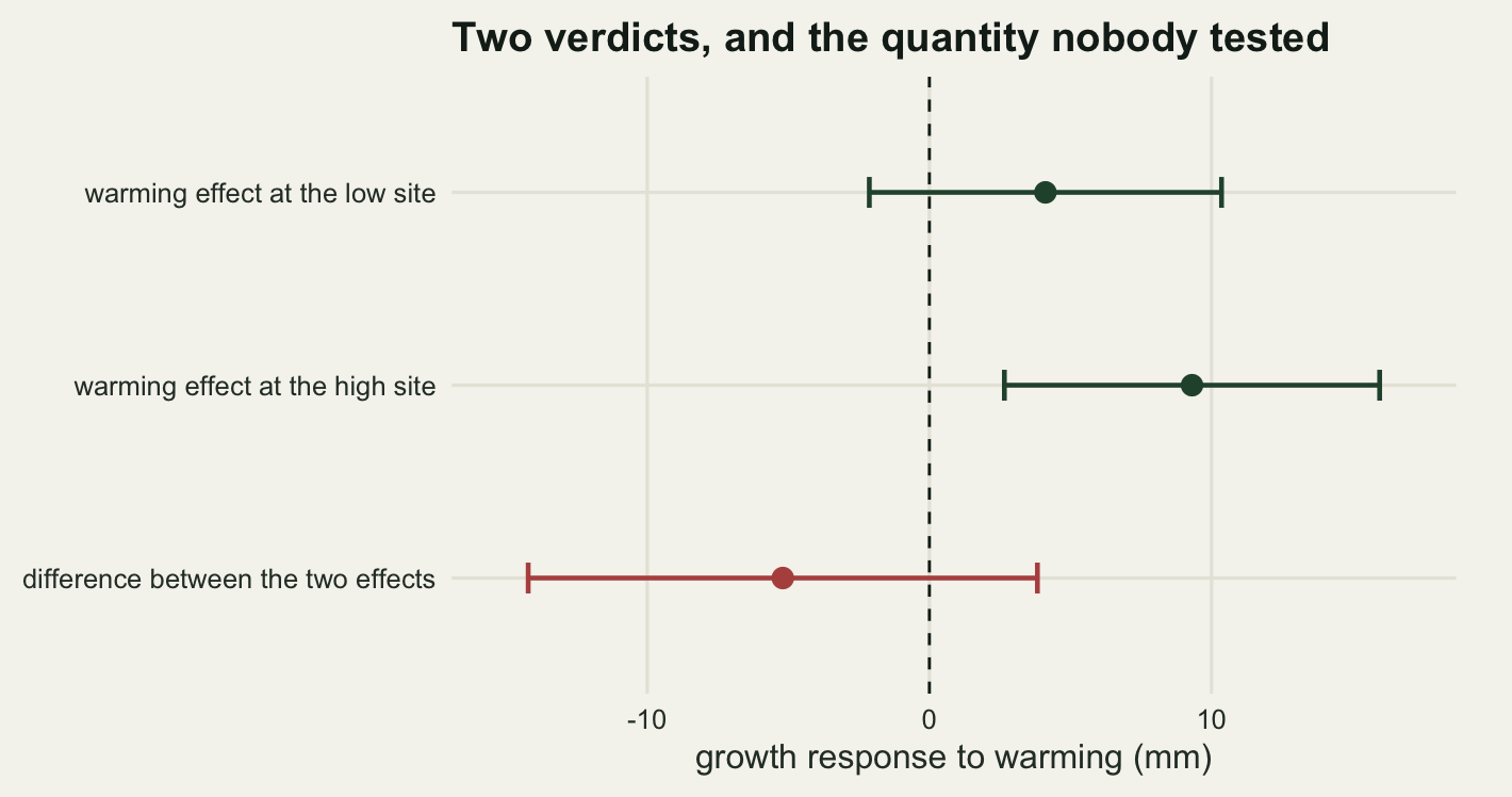
2 20260805 The loop needed 2 draws to find a split. The site that came out significant was the high one, p 0.0069, and the low site did not, p 0.1923. Written up in the ordinary way that reads as warming mattering above the treeline and not below it, with a ready mechanism about snow cover and season length waiting to be attached to it. The true effect is the same at both sites, and which site wins is a coin toss.
The interaction coefficient in the same fitted model is 5.196 millimetres with a standard error of 4.557 and a p value of 0.257. The test of the thing the discussion wants to claim was available in the same one-line model fit, and it says there is no evidence for the claim.
eff_of <- function(dd, which_site) {
  sub_dat <- dd[dd$site == which_site, ]
  tt <- t.test(growth ~ warming, data = sub_dat, var.equal = TRUE)
  c(est = unname(diff(tt$estimate)), lo = -tt$conf.int[2],
    hi = -tt$conf.int[1], p = tt$p.value)
}
e_low <- eff_of(dat, "low")
e_high <- eff_of(dat, "high")

se_low <- (e_low[["hi"]] - e_low[["lo"]]) / (2 * qt(0.975, 2 * n_cell - 2))
se_high <- (e_high[["hi"]] - e_high[["lo"]]) / (2 * qt(0.975, 2 * n_cell - 2))
se_gap <- sqrt(se_low^2 + se_high^2)
gap_est <- e_low[["est"]] - e_high[["est"]]

print(round(rbind(low = e_low, high = e_high), 4))
est lo hi p
low 4.1134 -2.1286 10.3553 0.1923
high 9.3090 2.6585 15.9595 0.0069print(round(c(se_low = se_low, se_high = se_high,
se_of_difference = se_gap,
sum_of_the_two_ses = se_low + se_high,
difference_mm = gap_est,
difference_in_its_own_se = gap_est / se_gap), 4)) se_low se_high se_of_difference
3.1183 3.3224 4.5566
sum_of_the_two_ses difference_mm difference_in_its_own_se
6.4407 -5.1957 -1.1403 Three numbers from that block carry the whole argument. The two site effects have standard errors of 3.118 and 3.322 millimetres. The difference between them has a standard error of 4.557, which is neither of those and is not their sum of 6.441 either. And the difference itself is -5.196 millimetres, which is 1.14 of its own standard errors: below the two it would need. The low site, the one that did not reach significance, in fact has the smaller estimated effect of the two, so the split verdict is at least pointing the way the point estimates point. It is pointing at a gap the data cannot resolve.
How often the verdicts split when nothing differs
One dataset settles nothing, so the whole design gets run four thousand times with the warming effect held identical at both sites. Each replicate draws four cells of thirty seedlings, runs the two within-site tests, and runs the interaction test on the same data. The simulator works on the cell means and the pooled sums of squares directly rather than calling lm four thousand times, which is the same arithmetic at a fraction of the cost.
sim_two_site <- function(seed, nc, d_low, d_high, n_rep, sg = sigma_r) {
  set.seed(seed)
  cell <- function(mu) {
    y <- matrix(rnorm(nc * n_rep, mu, sg), nc, n_rep)
    list(m = colMeans(y), ss = colSums((y - rep(colMeans(y), each = nc))^2))
  }
  a0 <- cell(0); a1 <- cell(d_low * sg)
  b0 <- cell(0); b1 <- cell(d_high * sg)
  dfw <- 2 * nc - 2
  dfi <- 4 * nc - 4
  s_low <- sqrt((a0$ss + a1$ss) / dfw)
  s_high <- sqrt((b0$ss + b1$ss) / dfw)
  s_pool <- sqrt((a0$ss + a1$ss + b0$ss + b1$ss) / dfi)
  e_lo <- a1$m - a0$m
  e_hi <- b1$m - b0$m
  se_lo <- s_low * sqrt(2 / nc)
  se_hi <- s_high * sqrt(2 / nc)
  se_dif <- s_pool * sqrt(4 / nc)
  data.frame(e_lo = e_lo, se_lo = se_lo,
             p_lo = 2 * pt(-abs(e_lo / se_lo), dfw),
             e_hi = e_hi, se_hi = se_hi,
             p_hi = 2 * pt(-abs(e_hi / se_hi), dfw),
             e_dif = e_lo - e_hi, se_dif = se_dif,
             p_dif = 2 * pt(-abs((e_lo - e_hi) / se_dif), dfi))
}

n_rep_main <- 4000
run_null <- sim_two_site(20260804, n_cell, d_true, d_true, n_rep_main)
sig_lo <- run_null$p_lo < 0.05
sig_hi <- run_null$p_hi < 0.05

rate_one <- mean(xor(sig_lo, sig_hi))
rate_both <- mean(sig_lo & sig_hi)
rate_none <- mean(!sig_lo & !sig_hi)
rate_int <- mean(run_null$p_dif < 0.05)
pow_site <- mean(c(sig_lo, sig_hi))

print(round(c(replicates = n_rep_main,
              power_per_site = pow_site,
              significant_at_exactly_one = rate_one,
              significant_at_both = rate_both,
              significant_at_neither = rate_none,
              interaction_test_rejects = rate_int), 5))
replicates power_per_site
4000.00000 0.47513
significant_at_exactly_one significant_at_both
0.50225 0.22400
significant_at_neither interaction_test_rejects
0.27375 0.04700 print(round(c(two_p_one_minus_p = 2 * pow_site * (1 - pow_site),
mc_se_of_rate_one = sqrt(rate_one * (1 - rate_one) / n_rep_main),
mc_se_of_rate_int = sqrt(rate_int * (1 - rate_int) / n_rep_main)),
5))two_p_one_minus_p mc_se_of_rate_one mc_se_of_rate_int
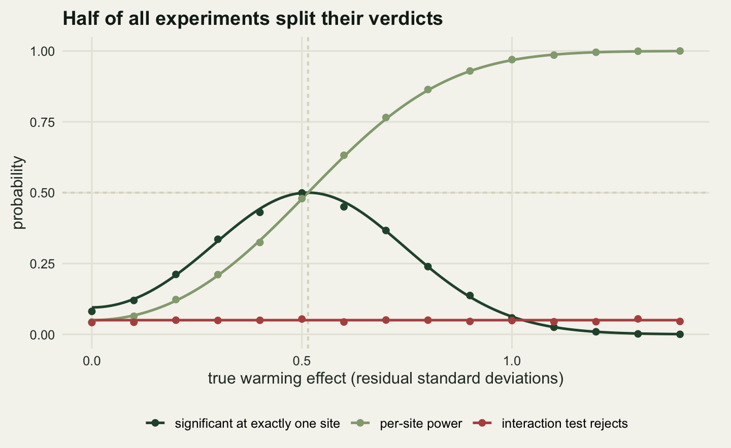
0.49876 0.00791 0.00335 With the true effect identical at both sites, the two within-site tests give different verdicts in 50.22 per cent of experiments. That is the headline number. Half of all such studies produce the raw material for a sentence about the response depending on elevation, in a world where it does not depend on elevation at all.
The value is not a coincidence of this design. Each site’s test rejects with probability 0.4751, and the two tests are independent because they use different seedlings, so the chance that exactly one of them rejects is \(2p(1-p) =\) 0.4988, against the measured 0.5022 with a Monte Carlo standard error of 0.0079. The function \(2p(1-p)\) has its maximum at \(p = 1/2\) and its maximum value is one half, so no design can push this above fifty per cent, and any design whose per-site power sits anywhere near one half is close to the worst case.
Meanwhile the interaction test on the same four thousand datasets rejects 4.7 per cent of the time, against a nominal five. It is not that the correct test is unavailable or hard. It is sitting in the same model fit, doing exactly what it is supposed to do, while the comparison of verdicts runs at ten times its error rate.
The rate depends on power, and it peaks where designs live
If the split-verdict rate is \(2p(1-p)\) then it is a function of per-site power alone, which means it can be traced across the whole range of true effect sizes. At a true effect of zero both tests reject at five per cent, so the split rate is about a tenth. At a large true effect both tests reject almost always, so the split rate falls back towards zero. In between there is a maximum, and the maximum is exactly where a well-designed but not lavishly funded ecological experiment tends to sit.
pow_within <- function(d, nc) {
  dfw <- 2 * nc - 2
  tc <- qt(0.975, dfw)
  ncp <- d * sqrt(nc / 2)
  pt(-tc, dfw, ncp) + pt(tc, dfw, ncp, lower.tail = FALSE)
}

d_grid <- seq(0, 1.4, by = 0.1)
n_rep_curve <- 2000
curve_tab <- as.data.frame(t(vapply(seq_along(d_grid), function(j) {
  rr <- sim_two_site(31000 + j, n_cell, d_grid[j], d_grid[j], n_rep_curve)
  a <- rr$p_lo < 0.05
  b <- rr$p_hi < 0.05
  c(d = d_grid[j], power = mean(c(a, b)), one = mean(xor(a, b)),
    both = mean(a & b), inter = mean(rr$p_dif < 0.05))
}, numeric(5))))
curve_tab$power_th <- pow_within(curve_tab$d, n_cell)
curve_tab$one_th <- 2 * curve_tab$power_th * (1 - curve_tab$power_th)
print(round(curve_tab, 4))
d power one both inter power_th one_th
1 0.0 0.0435 0.0810 0.0030 0.0415 0.0500 0.0950
2 0.1 0.0638 0.1195 0.0040 0.0425 0.0668 0.1246
3 0.2 0.1227 0.2115 0.0170 0.0500 0.1187 0.2092
4 0.3 0.2108 0.3355 0.0430 0.0490 0.2079 0.3293
5 0.4 0.3242 0.4305 0.1090 0.0495 0.3315 0.4432
6 0.5 0.4790 0.4990 0.2295 0.0540 0.4779 0.4990
7 0.6 0.6320 0.4500 0.4070 0.0435 0.6275 0.4675
8 0.7 0.7652 0.3665 0.5820 0.0505 0.7599 0.3649
9 0.8 0.8640 0.2390 0.7445 0.0500 0.8614 0.2387
10 0.9 0.9295 0.1370 0.8610 0.0455 0.9289 0.1321
11 1.0 0.9695 0.0580 0.9405 0.0485 0.9677 0.0625
12 1.1 0.9855 0.0250 0.9730 0.0445 0.9871 0.0255
13 1.2 0.9955 0.0090 0.9910 0.0445 0.9955 0.0090
14 1.3 0.9992 0.0015 0.9985 0.0545 0.9986 0.0028
15 1.4 1.0000 0.0000 1.0000 0.0455 0.9996 0.0007d_half <- uniroot(function(x) pow_within(x, n_cell) - 0.5, c(0.05, 1.5))$root
peak_row <- curve_tab[which.max(curve_tab$one), ]
print(round(c(d_where_power_is_half = d_half,
effect_mm_there = d_half * sigma_r,
measured_peak_d = peak_row$d,
measured_peak_rate = peak_row$one,
interaction_rate_mean = mean(curve_tab$inter),
interaction_rate_min = min(curve_tab$inter),
interaction_rate_max = max(curve_tab$inter)), 4))d_where_power_is_half effect_mm_there measured_peak_d
0.5146 6.1751 0.5000
measured_peak_rate interaction_rate_mean interaction_rate_min
0.4990 0.0476 0.0415
interaction_rate_max
0.0545 The measured curve peaks at a true effect of 0.5 standard deviations with a split-verdict rate of 0.499, and the closed form puts per-site power at one half at 0.5146 standard deviations, which for this residual variation is 6.175 millimetres of growth. Either side of that the rate falls, but it falls slowly: anywhere between about three tenths and seven tenths of a standard deviation of true effect, the split-verdict rate is above thirty per cent.
The interaction test is flat across the whole sweep, averaging 0.0476 and never leaving the band from 0.0415 to 0.0545. It has to be flat, because the true interaction is zero at every point on the curve. That is the contrast worth holding on to: one procedure has a false-positive rate that moves from ten per cent to fifty per cent and back depending on how big the common effect happens to be, and the other has a false-positive rate of five per cent regardless.
What the overlapping-error-bars rule really tests
The graphical version of the fallacy is older and more common than the p value version. Two means with 95 per cent intervals go on a figure, the intervals do not overlap, and the caption or the reader treats that as a significant difference. Schenker and Gentleman (2001) worked out what that rule actually does, and the arithmetic is short enough to redo here.
Two independent estimates \(\hat\theta_1\) and \(\hat\theta_2\) have standard errors \(s_1\) and \(s_2\). Their difference has a standard error of
\[s_{\text{diff}} = \sqrt{s_1^2 + s_2^2}\]
which is the only line of algebra this post needs, and it is the line Altman and Bland (2003) built their note around. The intervals fail to overlap when the gap between the estimates exceeds \(1.96(s_1 + s_2)\). The difference is significant at five per cent when the gap exceeds \(1.96\sqrt{s_1^2 + s_2^2}\). Since a sum of two positive numbers is always at least as large as the square root of their sum of squares, the non-overlap rule is always the stricter of the two, and how much stricter depends only on how the two standard errors compare.
ratio_grid <- c(1, 0.7, 0.5, 0.35, 0.25, 0.17, 0.1, 0.05, 0)
strict_fac <- (1 + ratio_grid) / sqrt(1 + ratio_grid^2)
alpha_impl <- 2 * pnorm(-1.96 * strict_fac)
print(round(rbind(se_ratio = ratio_grid,
                  standard_errors_demanded = 1.96 * strict_fac,
                  implied_alpha = alpha_impl), 5))
[,1] [,2] [,3] [,4] [,5] [,6]
se_ratio 1.00000 0.70000 0.50000 0.35000 0.25000 0.17000
standard_errors_demanded 2.77186 2.72968 2.62962 2.49745 2.37685 2.26076
implied_alpha 0.00557 0.00634 0.00855 0.01251 0.01746 0.02377
[,7] [,8] [,9]
se_ratio 0.10000 0.05000 0.00
standard_errors_demanded 2.14530 2.05543 1.96
implied_alpha 0.03193 0.03984 0.05alpha_equal <- 2 * pnorm(-1.96 * sqrt(2))
print(round(c(equal_precision_factor = sqrt(2),
equal_precision_demand = 1.96 * sqrt(2),
equal_precision_alpha = alpha_equal,
nominal_alpha = 0.05,
ratio_of_alphas = 0.05 / alpha_equal), 5))equal_precision_factor equal_precision_demand equal_precision_alpha
1.41421 2.77186 0.00557
nominal_alpha ratio_of_alphas
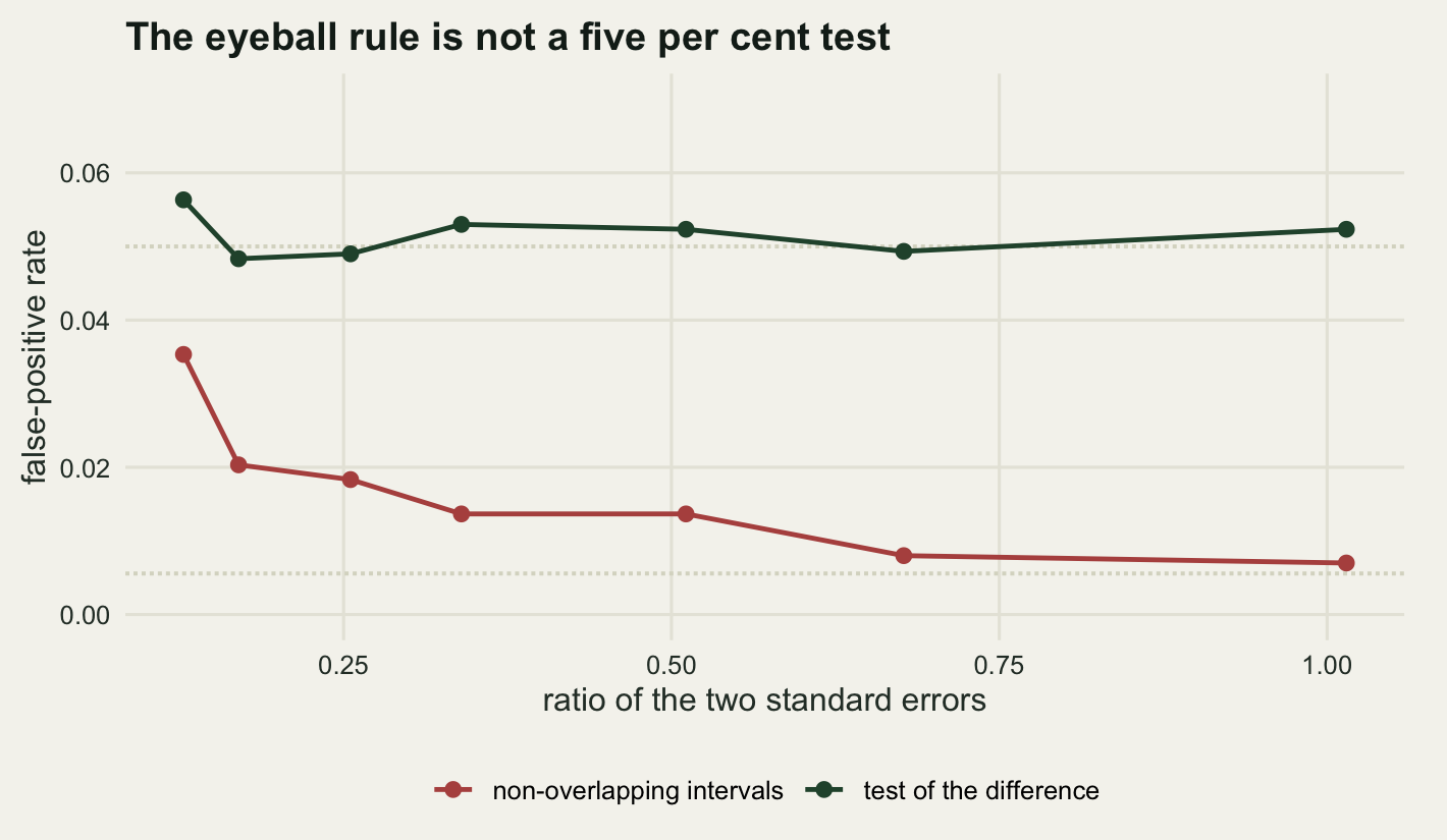
0.05000 8.97066 When the two estimates are equally precise, \(s_1 = s_2\), the factor is \(\sqrt{2} =\) 1.4142, so the non-overlap rule demands a gap of 2.772 standard errors where the five per cent test demands 1.96. That is a test at the 0.0056 level, which is 8.97 times stricter than the one the reader thinks is being applied. At the other extreme, when one estimate is far more precise than the other, the factor tends to one and the rule converges on the nominal five per cent from below.
That is worth being clear about, because the direction surprises people who expect an eyeball rule to be too permissive. Non-overlapping intervals are strong evidence of a real difference. The failure is the other way round: intervals that overlap, sometimes by a lot, routinely hide a difference that a proper test would call significant. The rule is conservative as a detector of differences and it is that conservatism, not any looseness, that makes it useless in the split-verdict situation, where the whole question is about a difference the eye has already decided is absent.
sim_pair <- function(seed, n_a, n_b, d_a, d_b, n_rep, sg = sigma_r) {
  set.seed(seed)
  cell <- function(nn, mu) {
    y <- matrix(rnorm(nn * n_rep, mu, sg), nn, n_rep)
    list(m = colMeans(y), ss = colSums((y - rep(colMeans(y), each = nn))^2))
  }
  a0 <- cell(n_a, 0); a1 <- cell(n_a, d_a * sg)
  b0 <- cell(n_b, 0); b1 <- cell(n_b, d_b * sg)
  e_a <- a1$m - a0$m
  e_b <- b1$m - b0$m
  se_a <- sqrt((a0$ss + a1$ss) / (2 * n_a - 2)) * sqrt(2 / n_a)
  se_b <- sqrt((b0$ss + b1$ss) / (2 * n_b - 2)) * sqrt(2 / n_b)
  dfd <- 2 * n_a + 2 * n_b - 4
  s_pool <- sqrt((a0$ss + a1$ss + b0$ss + b1$ss) / dfd)
  se_d <- s_pool * sqrt(2 / n_a + 2 / n_b)
  ta <- qt(0.975, 2 * n_a - 2)
  tb <- qt(0.975, 2 * n_b - 2)
  lo_a <- e_a - ta * se_a; hi_a <- e_a + ta * se_a
  lo_b <- e_b - tb * se_b; hi_b <- e_b + tb * se_b
  data.frame(no_overlap = as.numeric(lo_a > hi_b | lo_b > hi_a),
             diff_rejects = as.numeric(2 * pt(-abs((e_a - e_b) / se_d), dfd) < 0.05),
             se_ratio = se_b / se_a)
}

n_ref <- 20
n_other <- c(20, 45, 80, 180, 320, 720, 1280)
n_rep_ov <- 3000
ov_tab <- as.data.frame(t(vapply(seq_along(n_other), function(j) {
  rr <- sim_pair(52000 + j, n_ref, n_other[j], d_true, d_true, n_rep_ov)
  rat <- mean(rr$se_ratio)
  c(n_second_site = n_other[j], se_ratio = rat,
    non_overlap_rate = mean(rr$no_overlap),
    difference_test_rate = mean(rr$diff_rejects),
    normal_theory = 2 * pnorm(-1.96 * (1 + rat) / sqrt(1 + rat^2)))
}, numeric(5))))
print(round(ov_tab, 5))
n_second_site se_ratio non_overlap_rate difference_test_rate normal_theory
1 20 1.01469 0.00700 0.05233 0.00557
2 45 0.67718 0.00800 0.04933 0.00649
3 80 0.51108 0.01367 0.05233 0.00836
4 180 0.33981 0.01367 0.05300 0.01290
5 320 0.25527 0.01833 0.04900 0.01713
6 720 0.16988 0.02033 0.04833 0.02379
7 1280 0.12790 0.03533 0.05633 0.02832print(round(c(non_overlap_at_equal_precision = ov_tab$non_overlap_rate[1],
non_overlap_most_unequal = ov_tab$non_overlap_rate[nrow(ov_tab)],
difference_test_mean = mean(ov_tab$difference_test_rate),
nominal = 0.05), 5))non_overlap_at_equal_precision non_overlap_most_unequal
0.00700 0.03533
difference_test_mean nominal
0.05152 0.05000 The simulation holds the true effect equal at the two sites and varies only how many seedlings the second site has, from 20 per arm up to 1280, which drives the ratio of the two standard errors from 1.015 down to 0.128. At equal precision the non-overlap rule fires in 0.7 per cent of experiments, close to the 0.557 per cent that the normal-theory calculation predicts and a long way below five. At the most unequal precision tested it fires in 3.53 per cent, climbing towards the nominal rate as the arithmetic says it should. The properly constructed test of the difference sits at 5.15 per cent across the whole sweep, which is what a five per cent test is meant to do.
The failure also runs the other way
Split verdicts manufacture differences that are not there. The mirror image manufactures sameness: two sites whose warming responses genuinely differ, where both within-site tests happen to reject, and the paper reports that warming increased growth at both sites and says nothing about the difference. Or both fail to reject, and the paper says warming did nothing anywhere. Either way the difference goes unreported, and it is a difference the data could have detected.
The setting for this one has a real interaction. Warming is worth a full standard deviation at the low site and 0.45 of one at the high site, with sixty seedlings a cell rather than thirty, so both sites have decent power and the difference is detectable.
d_low_r <- 1.0
d_high_r <- 0.45
n_rev <- 60
run_rev <- sim_two_site(64000, n_rev, d_low_r, d_high_r, n_rep_main)
r_lo <- run_rev$p_lo < 0.05
r_hi <- run_rev$p_hi < 0.05
r_int <- run_rev$p_dif < 0.05

print(round(c(true_effect_low = d_low_r, true_effect_high = d_high_r,
              true_difference = d_low_r - d_high_r,
              seedlings_per_cell = n_rev,
              power_low_site = mean(r_lo), power_high_site = mean(r_hi),
              power_of_interaction_test = mean(r_int)), 5))
true_effect_low true_effect_high true_difference
1.00000 0.45000 0.55000
seedlings_per_cell power_low_site power_high_site
60.00000 0.99950 0.67450
power_of_interaction_test
0.55875 print(round(c(verdicts_agree = mean(r_lo == r_hi),
agree_and_interaction_rejects = mean((r_lo == r_hi) & r_int),
both_significant_and_interaction_rejects = mean(r_lo & r_hi & r_int),
neither_significant_and_interaction_rejects =
mean(!r_lo & !r_hi & r_int)), 5)) verdicts_agree
0.67500
agree_and_interaction_rejects
0.27575
both_significant_and_interaction_rejects
0.27575
neither_significant_and_interaction_rejects
0.00000 print(round(c(p_interaction_given_split = mean(r_int[xor(r_lo, r_hi)]),
p_interaction_given_both = mean(r_int[r_lo & r_hi]),
split_and_interaction_does_not_reject =
mean(xor(r_lo, r_hi) & !r_int)), 5)) p_interaction_given_split p_interaction_given_both
0.87077 0.40882
split_and_interaction_does_not_reject
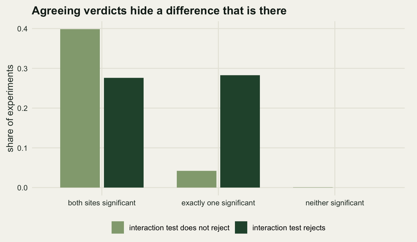
0.04200 The two within-site tests agree in 67.5 per cent of these experiments, and in 27.58 per cent of them they agree while the interaction test rejects. Rather more than a quarter of the studies in this scenario carry a detectable difference between the sites that the comparison-of-verdicts reading throws away, because the reader sees two asterisks and stops.
All of that agreement is of one kind. The low site has power 0.9995 here, so the case where both sites come out non-significant occurs in 0.05 per cent of replicates and contributes 0 per cent to the hidden-difference total. The both-significant route is the one that matters at this sample size; the both-non-significant route belongs to smaller studies, where it becomes the standard way a real interaction is written up as no effect anywhere.
The conditional rates are worth reading in both directions. Given that the verdicts split, the interaction test rejects 87.08 per cent of the time here, so in a scenario with a real and sizeable interaction a split verdict is often pointing at something. Given that both sites came out significant, it still rejects 40.88 per cent of the time. Neither conditional rate is anywhere near zero or one, which is the practical statement: the pattern of verdicts carries some information about the interaction and it is nothing like a substitute for testing it.
Testing the difference, two ways that agree
The correct procedure is one term in one model. Fit growth on warming, site and their interaction, and the interaction coefficient is the difference between the two site-specific warming effects, with a standard error that already accounts for both.
The second way is worth doing by hand even though it gives the same answer, because it generalises to every question the coefficient table does not happen to answer directly. Write the quantity you want as a weighted sum of the coefficients, \(k^{\top}\beta\), put the weights in a vector \(k\), and take the standard error from the model’s variance-covariance matrix, \(\sqrt{k^{\top}\,\mathrm{Var}(\hat\beta)\,k}\), which vcov returns for any fitted model in R. No extra package is needed for this.
contrast_of <- function(model, weights, dfree = model$df.residual) {
  bv <- coef(model)
  kv <- rep(0, length(bv))
  names(kv) <- names(bv)
  kv[names(weights)] <- weights
  est <- sum(kv * bv)
  se <- sqrt(drop(t(kv) %*% vcov(model) %*% kv))
  c(estimate = est, se = se, t = est / se,
    p = 2 * pt(-abs(est / se), dfree))
}

print(names(coef(fit_full)))
[1] "(Intercept)" "warmingwarmed" "sitehigh"
[4] "warmingwarmed:sitehigh"k_low <- c(warmingwarmed = 1)
k_high <- c(warmingwarmed = 1, `warmingwarmed:sitehigh` = 1)
k_gap <- c(`warmingwarmed:sitehigh` = -1)
ctab <- rbind(effect_at_low = contrast_of(fit_full, k_low),
effect_at_high = contrast_of(fit_full, k_high),
low_minus_high = contrast_of(fit_full, k_gap))
print(round(ctab, 6)) estimate se t p
effect_at_low 4.113381 3.221968 1.276667 0.204270
effect_at_high 9.309039 3.221968 2.889240 0.004610
low_minus_high -5.195658 4.556551 -1.140261 0.256526print(round(summary(fit_full)$coefficients["warmingwarmed:sitehigh", ], 6)) Estimate Std. Error t value Pr(>|t|)
5.195658 4.556551 1.140261 0.256526 print(round(c(contrast_t = unname(ctab["low_minus_high", "t"]),
interaction_t = unname(summary(fit_full)$coefficients[4, 3]),
absolute_gap = abs(abs(ctab["low_minus_high", "t"]) -
abs(summary(fit_full)$coefficients[4, 3]))), 12)) contrast_t interaction_t absolute_gap
-1.140261 1.140261 0.000000 The hand-built contrast and the interaction row of the coefficient table have the same absolute t value, the difference between the two rounded to 12 decimal places being 0. They differ only in sign, because the contrast was written as low minus high and the model’s treatment coding makes the interaction term high minus low. That is the whole content of the correct procedure: the model already contains the answer, and the contrast vector is a way of asking for it in the direction you meant.
One number in that table, the pooled standard error shared by both site rows, does not match the earlier within-site t tests, and the mismatch is instructive. The contrast puts the low-site effect at 4.1134 with a standard error of 3.222, while the separate t test on the low-site data gave a p value of 0.1923 against the contrast’s 0.2043. The estimates agree exactly and the standard errors do not, because the model pools the residual variance across all four cells and carries 116 degrees of freedom where the separate test carries 58. Pooling is an assumption, and if the two sites have genuinely different residual variation it is the wrong one.
The same two lines work on a GLM. Counts of surviving seedlings per plot, warming and site crossed, Poisson family: the interaction is now a ratio of ratios on the log link, and the contrast function needs only the change from a t distribution to a normal one.
mk_counts <- function(seed, nc, lam_low, lam_high, rr_low, rr_high) {
  set.seed(seed)
  site <- factor(rep(c("low", "high"), each = 2 * nc),
                 levels = c("low", "high"))
  warming <- factor(rep(rep(c("ambient", "warmed"), each = nc), 2),
                    levels = c("ambient", "warmed"))
  lam <- c(rep(lam_low, nc), rep(lam_low * rr_low, nc),
           rep(lam_high, nc), rep(lam_high * rr_high, nc))
  data.frame(site = site, warming = warming,
             seedlings = rpois(4 * nc, lam))
}

rr_true <- 1.35
cdat <- mk_counts(20260805, n_cell, 9, 5, rr_true, rr_true)
gfit <- glm(seedlings ~ warming * site, family = poisson, data = cdat)
print(round(summary(gfit)$coefficients, 4))
Estimate Std. Error z value Pr(>|z|)
(Intercept) 2.1972 0.0609 36.1041 0.0000
warmingwarmed 0.3258 0.0799 4.0801 0.0000
sitehigh -0.4804 0.0984 -4.8801 0.0000
warmingwarmed:sitehigh -0.1606 0.1321 -1.2162 0.2239contrast_g <- function(model, weights) {
bv <- coef(model)
kv <- rep(0, length(bv))
names(kv) <- names(bv)
kv[names(weights)] <- weights
est <- sum(kv * bv)
se <- sqrt(drop(t(kv) %*% vcov(model) %*% kv))
c(estimate = est, se = se, z = est / se,
p = 2 * pnorm(-abs(est / se)), rate_ratio = exp(est))
}
gtab <- rbind(low = contrast_g(gfit, k_low),
high = contrast_g(gfit, k_high),
ratio_of_ratios = contrast_g(gfit, k_gap))
print(round(gtab, 6)) estimate se z p rate_ratio
low 0.325834 0.079859 4.080102 0.000045 1.385185
high 0.165210 0.105186 1.570642 0.116266 1.179641
ratio_of_ratios 0.160624 0.132067 1.216232 0.223896 1.174243print(round(c(true_rate_ratio_both_sites = rr_true,
true_ratio_of_ratios = 1), 4))true_rate_ratio_both_sites true_ratio_of_ratios
1.35 1.00 The Poisson fit reproduces the fallacy in its own idiom. Warming multiplies counts by 1.35 at both sites by construction, so the true ratio of ratios is 1, yet the warming effect at the low site comes out at 0.000045 on the p value scale and the effect at the high site at 0.116. Split verdicts again, this time because the high site has fewer seedlings to start with and a Poisson count carries less information when the mean is smaller. The ratio of ratios is 1.1742 with a p value of 0.224, and the honest report is that these data do not distinguish the two sites’ responses.
What the correct test costs
Everyone who has made this error has a reason, and the reason is usually sound: the interaction test is less powerful than the within-site tests, so it does not reject, and the split verdict is right there offering a story. The size of that gap can be measured exactly.
The within-site effect is a difference of two cell means, with a standard error of \(\sigma\sqrt{2/n}\). The interaction is a difference of two such differences, with a standard error of \(\sigma\sqrt{4/n}\). So the interaction is estimated with \(\sqrt{2}\) times the standard error of a within-site effect at the same \(n\), and reaching a given power for a given true value therefore takes twice the seedlings per cell. Since the interaction needs four cells and the within-site test needs two, the total sample size ratio is four.
pow_inter <- function(d, nc) {
  dfi <- 4 * nc - 4
  tc <- qt(0.975, dfi)
  ncp <- d * sqrt(nc / 4)
  pt(-tc, dfi, ncp) + pt(tc, dfi, ncp, lower.tail = FALSE)
}

n_pow <- c(10, 15, 20, 30, 40, 60, 80, 100, 130, 160, 200, 260)
n_rep_pow <- 2000
pow_tab <- as.data.frame(t(vapply(seq_along(n_pow), function(j) {
  rr <- sim_two_site(77000 + j, n_pow[j], d_true, 0, n_rep_pow)
  c(n_per_cell = n_pow[j],
    within_sim = mean(rr$p_lo < 0.05), inter_sim = mean(rr$p_dif < 0.05),
    within_exact = pow_within(d_true, n_pow[j]),
    inter_exact = pow_inter(d_true, n_pow[j]))
}, numeric(5))))
print(round(pow_tab, 4))
n_per_cell within_sim inter_sim within_exact inter_exact
1 10 0.1885 0.1165 0.1851 0.1201
2 15 0.2615 0.1465 0.2624 0.1585
3 20 0.3180 0.1905 0.3379 0.1971
4 30 0.4745 0.2700 0.4779 0.2740
5 40 0.5980 0.3525 0.5981 0.3490
6 60 0.7835 0.4840 0.7753 0.4875
7 80 0.8805 0.6085 0.8816 0.6062
8 100 0.9450 0.7135 0.9404 0.7033
9 130 0.9795 0.8125 0.9801 0.8120
10 160 0.9910 0.8760 0.9938 0.8845
11 200 0.9990 0.9415 0.9988 0.9419
12 260 1.0000 0.9825 0.9999 0.9807n80_within <- uniroot(function(x) pow_within(d_true, x) - 0.8, c(5, 500))$root
n80_inter <- uniroot(function(x) pow_inter(d_true, x) - 0.8, c(5, 2000))$root
print(round(c(effect_tested = d_true,
n_per_cell_within = n80_within,
n_per_cell_interaction = n80_inter,
per_cell_ratio = n80_inter / n80_within,
total_within = 2 * ceiling(n80_within),
total_interaction = 4 * ceiling(n80_inter),
total_ratio = 4 * n80_inter / (2 * n80_within)), 4)) effect_tested n_per_cell_within n_per_cell_interaction
0.5000 63.7656 126.0657
per_cell_ratio total_within total_interaction
1.9770 128.0000 508.0000
total_ratio
3.9540 print(round(c(max_abs_sim_minus_exact_within =
max(abs(pow_tab$within_sim - pow_tab$within_exact)),
max_abs_sim_minus_exact_inter =
max(abs(pow_tab$inter_sim - pow_tab$inter_exact))), 4))max_abs_sim_minus_exact_within max_abs_sim_minus_exact_inter
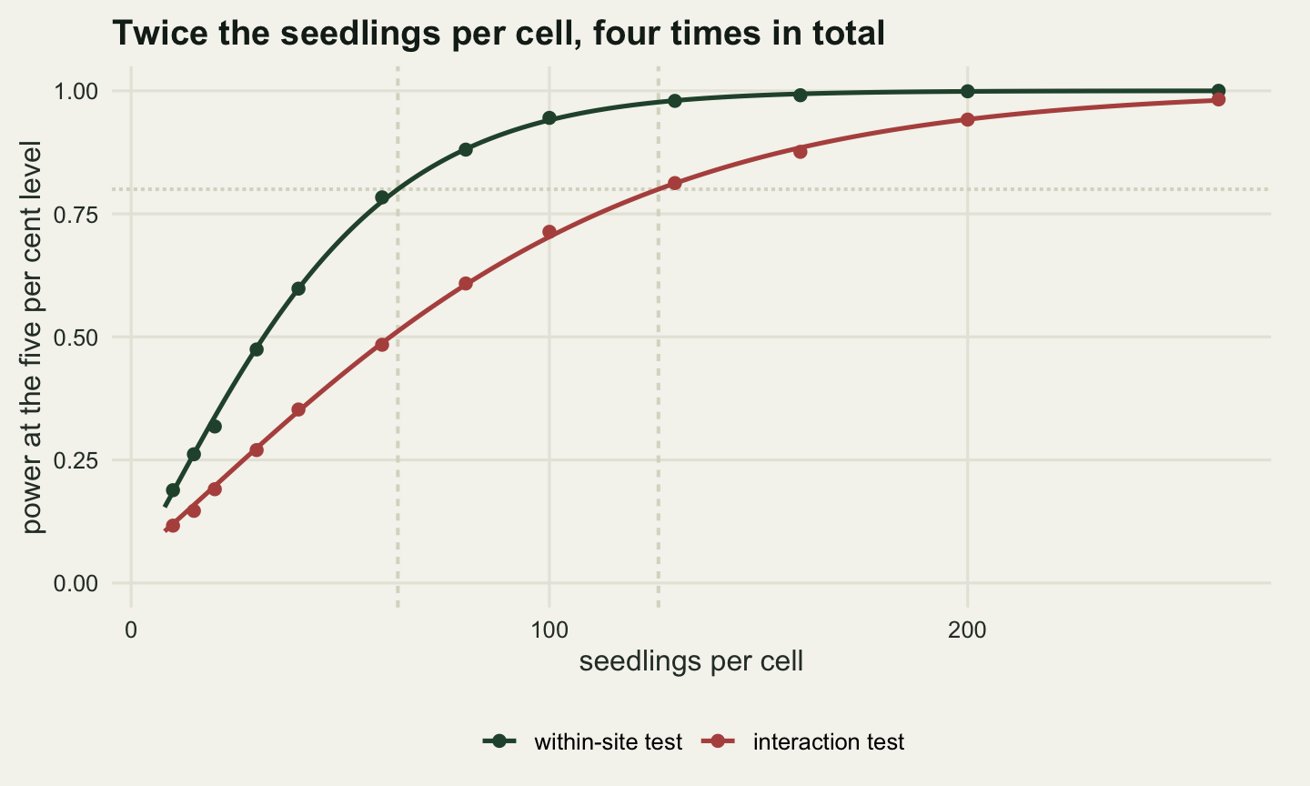
0.0199 0.0120 For a true effect of half a residual standard deviation, eighty per cent power needs 64 seedlings per arm at one site, which is 128 seedlings in total. Detecting a difference in warming effect of the same size between two sites needs 127 seedlings per cell, which is 508 seedlings in total. The per-cell ratio is 1.977 and the total ratio is 3.954, so the folk statement that an interaction costs four times the sample size is correct when it is read as total sample size, and the factor is two when it is read per cell. The simulated power never departs from the exact calculation by more than 0.0199.
That is the honest reason the fallacy is attractive, and it is also the reason it must not be used. An experiment powered to detect a warming effect is not powered to detect a difference in warming effects, and no amount of comparing verdicts changes that. The available responses are to design for the interaction if the interaction is the question, or to report the difference with its interval and say plainly that the data do not settle it. Nakagawa and Cuthill (2007) make the general version of that argument for biologists: report the estimate and its interval, and let the width of the interval say what the study can and cannot support.
There is a further trap on the low-power side. Gelman and Carlin (2014) point out that when power is low the estimates that clear the significance threshold are the ones that came out too large, and often the ones that came out with the wrong sign. A split verdict at low power therefore does not just fail to establish a difference: the site that won is the site whose estimate is most inflated, so the apparent difference between the two sites is larger than the truth even when a difference exists.
The honest limit: an interaction is a statement about a scale
Everything above treats the interaction test as the right answer, and within the model it is. What the model cannot supply is the scale on which the responses are being compared, and an interaction that exists on one scale can vanish on another. Loftus (1978) made the argument in a psychology journal and it transfers without modification: unless the measurement scale is fixed by something outside the statistics, the presence of an interaction is a property of the units as much as of the biology.
The demonstration is short. Let warming multiply growth by the same factor at both sites, which is a perfectly reasonable ecological hypothesis, and let the two sites differ in baseline growth, which they do. On the raw millimetre scale the two effects differ, because the same percentage of a larger baseline is a larger number of millimetres. On the log scale they are identical.
scale_sim <- function(seed, nc, b_low, b_high, rr, cv, n_rep) {
  set.seed(seed)
  cell <- function(mu) matrix(rlnorm(nc * n_rep, log(mu) - cv^2 / 2, cv),
                              nc, n_rep)
  a0 <- cell(b_low); a1 <- cell(b_low * rr)
  b0 <- cell(b_high); b1 <- cell(b_high * rr)
  int_rate <- function(m1, m2, m3, m4) {
    mats <- list(m1, m2, m3, m4)
    mm <- vapply(mats, colMeans, numeric(n_rep))
    ss <- 0
    for (k in 1:4) ss <- ss + colSums((mats[[k]] -
                                         rep(mm[, k], each = nc))^2)
    dfi <- 4 * nc - 4
    est <- (mm[, 2] - mm[, 1]) - (mm[, 4] - mm[, 3])
    se <- sqrt(ss / dfi) * sqrt(4 / nc)
    c(rate = mean(2 * pt(-abs(est / se), dfi) < 0.05),
      mean_est = mean(est))
  }
  c(raw = int_rate(a0, a1, b0, b1),
    logged = int_rate(log(a0), log(a1), log(b0), log(b1)))
}

sc_30 <- scale_sim(88000, 30, 46, 22, 1.35, 0.28, 3000)
sc_60 <- scale_sim(88001, 60, 46, 22, 1.35, 0.28, 3000)
print(round(rbind(n_30 = sc_30, n_60 = sc_60), 5))
raw.rate raw.mean_est logged.rate logged.mean_est
n_30 0.467 8.34691 0.05033 -0.00038
n_60 0.759 8.35933 0.05233 -0.00092print(round(c(baseline_low = 46, baseline_high = 22, ratio_both_sites = 1.35,
raw_effect_low_mm = 46 * 0.35, raw_effect_high_mm = 22 * 0.35,
raw_interaction_mm = (46 - 22) * 0.35,
log_interaction = 0), 4)) baseline_low baseline_high ratio_both_sites raw_effect_low_mm
46.00 22.00 1.35 16.10
raw_effect_high_mm raw_interaction_mm log_interaction
7.70 8.40 0.00 With thirty seedlings a cell the raw-scale interaction test rejects 46.7 per cent of the time and the log-scale test rejects 5.03 per cent. Double the sample and the raw-scale test rejects 75.9 per cent while the log-scale test stays at 5.23. Both tests are correct. They are testing different hypotheses, one about millimetres of extra growth and one about proportional growth, and the data cannot arbitrate between them. Running the interaction test does not make the elevation claim safe; it makes it precise, which is a different and smaller thing.
Ecotoxicology sets the same trap under different names: two stressors judged against an additive null on mortality and against a multiplicative null on survival can be called antagonistic by one comparison and synergistic by the other on the very same table, because the two nulls disagree about what acting independently means rather than about the counts. A logistic model’s interaction term, which lives on the log odds scale, is a third scale again, and it is free to disagree with both.
Three further limits are worth stating flatly. The open-top chamber design here has two sites, so elevation is confounded with everything else that differs between two mountainsides, and the interaction term estimates the difference between these two places rather than an effect of elevation. The simulation assumes equal residual variation at both sites, which is what lets the model pool; unequal variation makes the pooled interaction test wrong in a way the within-site Welch tests would not be, and the fix is a variance-per-site model rather than a return to comparing verdicts. And a non-significant interaction is not evidence that the two responses are the same. It is the absence of evidence that they differ, in a test whose sample size requirement is four times the one the study was designed around.
Where to go next
The immediate follow-on is the machinery, not the fallacy. The contrast vector built here took the narrowest case, two group-specific effects and their difference, and the same \(k^{\top}\beta\) with \(\sqrt{k^{\top}\mathrm{Var}(\hat\beta)k}\) answers every other question a coefficient table sidesteps: three sites rather than two, a comparison of slopes at chosen covariate values, an average of several cells against another average. Marginal means and contrasts after a GLM carries that through, including what to do about multiplicity once the number of contrasts stops being one.
If the interaction is going to be the question, it has to be in the design and not in the discussion, and reading a fitted interaction correctly is its own skill: the coefficient is a difference of slopes on the link scale and almost nobody reads it that way on first acquaintance. Interaction terms in ecological GLMs goes through that on count data.
The version of this problem that has nothing to do with interactions is a repeated-measures one. Comparing a before-and-after test in a treated group with a before-and-after test in a control group is the same error wearing different clothes, and the correct object there is also a difference of differences.
References
Gelman A, Stern H 2006 The American Statistician 60(4):328-331 (10.1198/000313006X152649)
Nieuwenhuis S, Forstmann BU, Wagenmakers EJ 2011 Nature Neuroscience 14(9):1105-1107 (10.1038/nn.2886)
Schenker N, Gentleman JF 2001 The American Statistician 55(3):182-186 (10.1198/000313001317097960)
Altman DG, Bland JM 2003 BMJ 326(7382):219 (10.1136/bmj.326.7382.219)
Nakagawa S, Cuthill IC 2007 Biological Reviews 82(4):591-605 (10.1111/j.1469-185X.2007.00027.x)
Gelman A, Carlin J 2014 Perspectives on Psychological Science 9(6):641-651 (10.1177/1745691614551642)
Loftus GR 1978 Memory and Cognition 6(3):312-319 (10.3758/BF03197461)