library(ggplot2)

te_paper  <- "#f5f4ee"
te_ink    <- "#16241d"
te_body   <- "#2c3a31"
te_forest <- "#275139"
te_rust   <- "#b5534e"
te_gold   <- "#c9b458"
te_line   <- "#dad9ca"

theme_datasheet <- function() {
  theme_minimal(base_size = 12) +
    theme(plot.background  = element_rect(fill = te_paper, colour = NA),
          panel.background = element_rect(fill = te_paper, colour = NA),
          panel.grid.major = element_line(colour = te_line, linewidth = 0.3),
          panel.grid.minor = element_blank(),
          text             = element_text(colour = te_body),
          plot.title       = element_text(colour = te_ink, face = "bold"),
          axis.text        = element_text(colour = te_body))
}

tost <- function(x, y, bound) {
  lo <- t.test(x, y, mu = -bound, alternative = "greater")$p.value
  hi <- t.test(x, y, mu =  bound, alternative = "less")$p.value
  max(lo, hi)
}Testing for no effect: equivalence tests in R
R
hypothesis testing
equivalence
study design
ecology tutorial
A non-significant p value is not evidence of no effect. Two one-sided tests give ecologists a procedure that can support absence, with a worked simulation in R.
A monitoring report says the treatment had no effect on beetle abundance. The evidence offered is a p value of 0.45. That is the wrong evidence, and every reviewer who has ever written “absence of evidence is not evidence of absence” in the margin is pointing at the same gap: the test was built to detect a difference, and it failed to. Failing to detect something is compatible with the thing being absent, and also with the study being too small to see it.
There is a procedure that supports the claim instead of dodging it. You state the smallest difference that would matter ecologically, and you test whether the true difference is smaller than that in both directions. Two one-sided tests, hence TOST. It is old, it is in base R, and it takes four lines.
The bound comes first
The part that is not statistical is the part that matters most. Equivalence testing needs a number: how large a difference would have to be before you would call it real, in the units of your response. Ten per cent of the control mean. Half a beetle per trap. One degree. That number is a biological judgement, and it has to be made before you look at the data, because it is what the whole procedure is calibrated against.
Once it exists, the arithmetic is simple. With bounds at plus and minus delta, run one t test against the lower bound and one against the upper, both one-sided, and take the larger of the two p values.
It is the confidence interval you already have
The TOST decision has an equivalent form that needs no new machinery at all. At the five per cent level, the two one-sided tests declare equivalence exactly when the ninety per cent confidence interval for the difference lies entirely between the bounds. Not the ninety-five per cent interval: the one-sided structure of the test means the relevant interval is the one with alpha in each tail rather than alpha over two.
That is worth checking rather than asserting, because the mismatch between the ninety and ninety-five is where readers usually slip.
set.seed(20260805)

one_pair <- function(n, delta, sd = 1) {
  list(x = rnorm(n, delta, sd), y = rnorm(n, 0, sd))
}

reps  <- 2000
bound <- 0.5
agree <- logical(reps)
for (i in seq_len(reps)) {
  d <- one_pair(n = 20, delta = runif(1, -1.5, 1.5))
  ci <- t.test(d$x, d$y, conf.level = 0.90)$conf.int
  agree[i] <- (tost(d$x, d$y, bound) < 0.05) ==
              (ci[1] > -bound && ci[2] < bound)
}
mean(agree)
[1] 1Over 2000 simulated comparisons the two rules agreed 100.00 per cent of the time. They are the same decision written two ways. If you already report an interval, you can read the equivalence verdict off it by eye, provided you widen your alpha to ten per cent first.
Four possible verdicts, not two
Running a difference test and an equivalence test together gives four outcomes, and ecologists meet all four. The pair of tests answers different questions, so they can both reject, both fail, or split either way.
verdict <- function(x, y, bound) {
  sig <- t.test(x, y)$p.value < 0.05
  eq  <- tost(x, y, bound) < 0.05
  if (sig && eq)  "both"
  else if (sig)   "difference only"
  else if (eq)    "equivalence only"
  else            "inconclusive"
}

set.seed(4242)
n_rep <- 2000
cells <- replicate(n_rep, {
  d <- one_pair(n = 40, delta = 0.3)
  verdict(d$x, d$y, bound = 0.5)
})
tab <- round(100 * table(factor(cells, levels = c("inconclusive", "equivalence only",
                                                  "difference only", "both"))) / n_rep, 1)
tab
    inconclusive equivalence only  difference only             both
            56.9             18.9             24.3              0.0
Forty observations per group, a true difference of 0.3 standard deviations, bounds at plus and minus 0.5. The study lands in the inconclusive cell 56.9 per cent of the time. It declares equivalence without significance 18.9 per cent of the time, and significance without equivalence 24.3 per cent. Both verdicts arrive together in 0.0 per cent of runs.
The inconclusive cell is the majority, and that is the honest description of a great many field studies. The data rule out neither a difference worth caring about nor a negligible one. Reporting that as “no effect” is the error the whole procedure exists to prevent.
The both cell is empty at this sample size, and it is worth saying why, because it is not a contradiction. A difference can be reliably present and still smaller than the smallest difference you said would matter. That is the most informative of the four outcomes, and no single test can produce it. Forty per group is simply too few to establish it here; the next figure shows where it appears.
n_grid <- c(10, 20, 40, 80, 200)
set.seed(77)
shares <- do.call(rbind, lapply(n_grid, function(nn) {
  v <- replicate(600, {
    d <- one_pair(n = nn, delta = 0.3)
    verdict(d$x, d$y, bound = 0.5)
  })
  p <- table(factor(v, levels = c("inconclusive", "equivalence only",
                                  "difference only", "both"))) / 600
  data.frame(n = nn, outcome = names(p), share = as.numeric(p))
}))
shares$outcome <- factor(shares$outcome,
                         levels = c("inconclusive", "equivalence only",
                                    "difference only", "both"))

ggplot(shares, aes(x = factor(n), y = share, fill = outcome)) +
  geom_col(width = 0.68) +
  scale_fill_manual(values = c("inconclusive" = te_line,
                               "equivalence only" = te_forest,
                               "difference only" = te_rust,
                               "both" = te_gold)) +
  scale_y_continuous(labels = function(v) paste0(100 * v, "%")) +
  labs(x = "observations per group", y = "share of studies", fill = NULL,
       title = "What a study of this size can conclude") +
  theme_datasheet() +
  theme(legend.position = "top")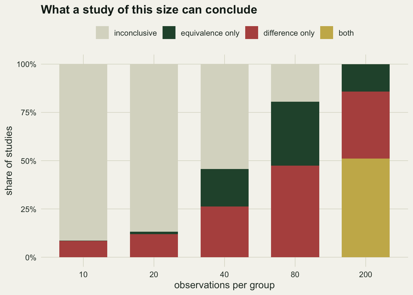
The figure makes the design consequence visible. A ten-per-group study is almost never able to say anything: it cannot detect the effect and it cannot rule it out. Both conclusions arrive with sample size, though not at the same pace, and at two hundred per group about half the studies report what is actually true of these data, which is a difference that is real and below the threshold that would matter.
The verdict moves with the bound
The bound is a decision, and decisions can be argued about, so the responsible way to report an equivalence test is to show what happens across a range of them. One data set, one sweep.
set.seed(21)
d <- one_pair(n = 40, delta = 0.15)
bounds <- seq(0.3, 1.1, by = 0.1)
sw <- data.frame(bound = bounds,
                 p = sprintf("%.4f", sapply(bounds, function(b) tost(d$x, d$y, b))),
                 equivalent = sapply(bounds, function(b) tost(d$x, d$y, b) < 0.05))
sw
bound p equivalent
1 0.3 0.3139 FALSE
2 0.4 0.1843 FALSE
3 0.5 0.0950 FALSE
4 0.6 0.0429 TRUE
5 0.7 0.0170 TRUE
6 0.8 0.0059 TRUE
7 0.9 0.0018 TRUE
8 1.0 0.0005 TRUE
9 1.1 0.0001 TRUEFor this single sample the observed difference is 0.184 and the plain t test gives p = 0.45, so by the usual reading the study found nothing. The equivalence verdict flips at a bound of 0.6: anything tighter and the data cannot rule out an effect of that size, anything looser and they can. A reader who thinks a difference of 0.4 would matter and a reader who only cares about differences above one standard deviation get opposite answers from the same experiment, correctly.
set.seed(303)
ex <- do.call(rbind, lapply(1:8, function(i) {
  nn <- c(20, 60, 200, 20, 60, 200, 60, 200)[i]
  dd <- one_pair(n = nn, delta = c(0, 0, 0.15, 0.4, 0.4, 0.25, 0.9, 0.9)[i])
  ci <- t.test(dd$x, dd$y, conf.level = 0.90)$conf.int
  data.frame(study = i, n = nn,
             est = mean(dd$x) - mean(dd$y),
             lo = ci[1], hi = ci[2],
             verdict = verdict(dd$x, dd$y, bound = 0.5))
}))
ex$label <- sprintf("n = %d", ex$n)

ggplot(ex, aes(y = factor(study), x = est, colour = verdict)) +
  geom_vline(xintercept = c(-0.5, 0.5), linetype = "dashed", colour = te_ink) +
  geom_vline(xintercept = 0, colour = te_line, linewidth = 0.6) +
  geom_errorbar(aes(xmin = lo, xmax = hi), orientation = "y",
                width = 0.28, linewidth = 0.7) +
  geom_point(size = 2.6) +
  geom_text(aes(x = max(ex$hi) + 0.12, label = label), hjust = 0, size = 3.2,
            colour = te_body, show.legend = FALSE) +
  scale_colour_manual(breaks = c("inconclusive", "equivalence only",
                                 "difference only", "both"),
                      values = c("inconclusive" = te_gold,
                                 "equivalence only" = te_forest,
                                 "difference only" = te_rust,
                                 "both" = te_ink)) +
  scale_x_continuous(breaks = seq(-0.5, 1.5, by = 0.5)) +
  coord_cartesian(xlim = c(min(ex$lo, -0.62), max(ex$hi) + 0.42)) +
  labs(x = "difference in means, with 90 per cent interval",
       y = "simulated study", colour = NULL,
       title = "Reading the equivalence verdict off the interval") +
  theme_datasheet() +
  theme(legend.position = "top")
Warning: Use of `ex$hi` is discouraged.
ℹ Use `hi` instead.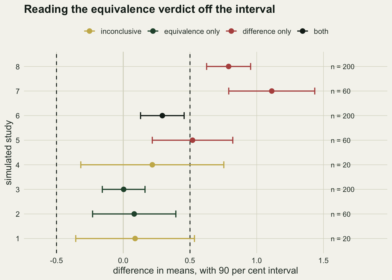
What to write in the paper
Three things, and they fit in one sentence each. The bound you chose and the biology behind it. The estimated difference with its ninety per cent interval. The TOST p value, or equivalently the statement that the interval does or does not sit inside the bounds. If the study is in the inconclusive cell, say so in those words: the data are compatible both with a difference worth caring about and with none.
That sentence is more useful to the next person than “no significant difference was found”, because it carries the size of the study with it.
Honest limits
TOST inherits every assumption of the test it is built on. The version here is a Welch t test on two independent samples, so it assumes independence and approximate normality of the sampling distribution of the mean, and nothing more; on strongly skewed counts you would build the same two one-sided tests around a GLM contrast or a bootstrap interval instead. The logic is unchanged, only the interval underneath it.
The bound is not a statistical quantity and cannot be estimated from the data. Choosing it after seeing the result, or setting it wide enough to guarantee a pass, converts the procedure into a rubber stamp. It should be preregistered or at least stated before the analysis, and the sweep above is the honest way to show a reader how much of the conclusion rests on it.
One design claim is worth checking rather than repeating: it is often said that declaring equivalence takes a much larger sample than detecting an effect of the same size. Across the sample sizes above the share of studies able to declare equivalence stays below the share able to detect the difference, and the gap does not close as the samples grow, so with this bound and this difference the claim points the right way: ruling the effect out takes the larger study. The real design lesson is the one in the stacked bars, which is that small studies conclude nothing either way.
Finally, equivalence at your bound is not equivalence full stop. It is a statement that the data are inconsistent with a difference larger than the number you nominated, at the confidence level you chose, in the response you measured. A treatment can be equivalent for abundance and not for body condition, and the test says nothing about the second.
References
Schuirmann DJ 1987 Journal of Pharmacokinetics and Biopharmaceutics 15(6):657-680 (10.1007/BF01068419)
Lakens D 2017 Social Psychological and Personality Science 8(4):355-362 (10.1177/1948550617697177)
Lakens D, Scheel AM, Isager PM 2018 Advances in Methods and Practices in Psychological Science 1(2):259-269 (10.1177/2515245918770963)