library(ggplot2)
library(patchwork)

te_paper  <- "#f5f4ee"
te_ink    <- "#16241d"
te_body   <- "#2c3a31"
te_forest <- "#275139"
te_rust   <- "#b5534e"
te_gold   <- "#c9b458"
te_line   <- "#dad9ca"

theme_datasheet <- function() {
  theme_minimal(base_size = 12) +
    theme(plot.background  = element_rect(fill = te_paper, colour = NA),
          panel.background = element_rect(fill = te_paper, colour = NA),
          panel.grid.major = element_line(colour = te_line, linewidth = 0.3),
          panel.grid.minor = element_blank(),
          text             = element_text(colour = te_body),
          plot.title       = element_text(colour = te_ink, face = "bold"),
          plot.subtitle    = element_text(colour = te_body),
          axis.text        = element_text(colour = te_body))
}NOEC rewards noisy toxicity tests
R
ecotoxicology
dose-response
hypothesis testing
simulation
ecology tutorial
The NOEC rises with residual scatter and falls with replication, while a fitted EC10 stays centred on the truth. Both measured on simulated toxicity tests in R.
Two contract laboratories run the same 72 hour algal growth inhibition test on the same substance. Both use a control and five concentrations, 2.5, 5, 10, 20 and 40 micrograms per litre, three replicate flasks at each, and both express growth rate as a percentage of the control. The first laboratory has tight flasks: its replicates scatter by about five per cent of the control mean. The second has older incubators and uneven light, and its replicates scatter by twenty. Both report a no-observed-effect concentration, the NOEC, and the second laboratory’s NOEC is higher. The substance looks safer in the worse experiment.
That is not an accident of one pair of tests. The NOEC is defined through a hypothesis test: it is the highest tested concentration that the test fails to separate from the control. Anything that lowers the power of the test, more scatter or fewer replicates, lets a larger real effect pass as no effect, and the NOEC climbs. Laskowski listed this among his reasons to abandon the NOEC in 1995, Crane and Newman asked what size of effect a NOEC actually hides, and Jager was still making the same case in 2012. This post measures it. The sweep is over residual scatter, replication and the number of concentrations, and it scores the NOEC against the one quantity it is usually compared with, the concentration that reduces the response by ten per cent, the EC10, read off the same true curve. The regression EC10 is fitted to the same simulated tests alongside it.
The argument is the institutional version of one this site has already made. Testing for no effect shows on a single comparison that a non-significant p value is not evidence of no effect, and that an equivalence test is the procedure that can support absence. The NOEC is that mistake turned into a regulatory endpoint, repeated across a concentration series and then reported as a concentration. Confidence intervals for effective doses and checking a dose-response analysis work on fitted effective doses: the first on what the delta, Fieller and profile intervals cover and where the concentrations should go, the second on the checks a fitted curve needs, including extrapolation below the lowest tested dose. Neither looks at a hypothesis test endpoint. Contrasts and post-hoc comparisons covers the corrections for testing every pair of groups, Tukey, Bonferroni and Holm among them, and ends one reading with the lowest dose “not separable from the control”. A NOEC is built from exactly that kind of verdict, restricted to the comparisons against the control; here the verdict is repeated thousands of times and turned into a concentration.
The NOEC as a test result
The true response is a three parameter log-logistic curve: growth as a percentage of control equals 100 divided by one plus the concentration over the EC50, raised to the slope. The EC50 is 16 micrograms per litre and the slope is 2. Every design constant in the post is fixed in the next chunk and none was changed after the simulations ran.
top_true   <- 100
ec50_true  <- 16
slope_true <- 2
conc_grid  <- c(2.5, 5, 10, 20, 40)
alpha_lev  <- 0.05

curve_mean <- function(conc) top_true / (1 + (conc / ec50_true)^slope_true)
effect_at  <- function(conc) 1 - curve_mean(conc) / top_true
ec10_true  <- ec50_true * (1 / 9)^(1 / slope_true)
eff_grid   <- 100 * effect_at(conc_grid)
next_above <- min(conc_grid[conc_grid > ec10_true])
The true EC10 is 5.33 micrograms per litre. The true reductions at the five tested concentrations are 2.4, 8.9, 28.1, 61.0 and 86.2 per cent. The EC10 falls between the second and third tested concentrations, so on this grid “the NOEC lies above the true EC10” and “the NOEC is 10 or higher” are the same event. That equivalence is a property of the grid, and the last section changes the grid.
The definition used by the critics cited here, and by the test guidelines they criticise, takes the lowest observed effect concentration, the LOEC, as the lowest tested concentration at which the test detects an effect, and the NOEC as the tested concentration immediately below it. For a continuous response with a control group the standard many-to-one procedure is Dunnett’s test, which compares each concentration with the control while holding the familywise error rate at the stated level. Dunnett’s critical value is the upper quantile of the maximum of several t statistics that share the control mean and the pooled variance, so they are correlated with correlation one half when the groups are equal in size. It has no closed form, and the usual route in R goes through a multivariate t package. The chunk below computes it directly instead. Given the standardised control mean and the ratio of the pooled standard deviation to the true one, the comparisons are independent, so the coverage is a two dimensional integral of a normal distribution function raised to the number of concentrations.
dunnett_crit <- function(k_conc, df_res, alpha = alpha_lev) {
  z_nodes <- seq(-8, 8, by = 0.05)
  w_z     <- dnorm(z_nodes) * 0.05
  u_nodes <- seq(0.005, 4, by = 0.01)
  w_u     <- dchisq(df_res * u_nodes^2, df_res) * 2 * df_res * u_nodes * 0.01
  coverage <- function(cc) {
    inner <- pnorm(outer(z_nodes, cc * sqrt(2) * u_nodes, "+"))^k_conc
    sum(w_z * (inner %*% w_u))
  }
  uniroot(function(cc) coverage(cc) - (1 - alpha), c(1, 6), tol = 1e-7)$root
}

crit_5_12  <- dunnett_crit(5, 12)
crit_5_inf <- dunnett_crit(5, 5000)
crit_1_12  <- dunnett_crit(1, 12)
t_1_12     <- qt(1 - alpha_lev, 12)

n_null <- 20000
n_null_per <- 3
set.seed(4102)
y_null <- array(rnorm(n_null * 6 * n_null_per, top_true, 10),
                c(n_null, 6, n_null_per))
gm_null <- rowMeans(y_null, dims = 2)
sp_null <- sqrt(rowMeans(apply(y_null, c(1, 2), var)))
t_null  <- (gm_null[, 1] - gm_null[, -1]) / (sp_null * sqrt(2 / n_null_per))
fwer_null <- mean(apply(t_null >= crit_5_12, 1, any))
fwer_se   <- sqrt(fwer_null * (1 - fwer_null) / n_null)
Three checks show the integral is the right one. With one comparison it must reduce to Student’s t, and it returns 1.7823 against qt() at 1.7823. For five concentrations and 12 residual degrees of freedom, which is the three replicate design here, it returns 2.502, and with the degrees of freedom sent towards infinity it returns 2.234; Dunnett’s 1955 one-sided table gives 2.50 and 2.23 for those two cases. Finally, in 20000 simulated tests with no effect at any concentration, at least one comparison was declared significant in 0.0508 of them (Monte Carlo standard error 0.0016), against the nominal 0.05.
noec_readings <- function(y_arr, conc, n_per) {
  k_conc <- length(conc)
  df_res <- (k_conc + 1) * (n_per - 1)
  crit   <- dunnett_crit(k_conc, df_res)
  g_mean <- rowMeans(y_arr, dims = 2)
  s_pool <- sqrt(rowMeans(apply(y_arr, c(1, 2), var)))
  t_dec  <- (g_mean[, 1] - g_mean[, -1]) / (s_pool * sqrt(2 / n_per))
  sig    <- t_dec >= crit
  # LOEC = lowest significant concentration; NOEC = the one below it
  first_sig <- max.col(cbind(sig, TRUE), ties.method = "first")
  noec_low  <- c(0, conc, conc[k_conc])[first_sig]
  # top-down reading: from the top, stop at the first non-significant
  top_run   <- max.col(cbind(!sig[, k_conc:1, drop = FALSE], TRUE),
                       ties.method = "first")
  noec_down <- c(rev(conc), 0)[top_run]
  # Holm on the same one-sided t statistics
  p_one  <- pt(t_dec, df_res, lower.tail = FALSE)
  p_sort <- t(apply(p_one, 1, sort))
  p_ord  <- t(apply(p_one, 1, order))
  holm_m <- t(apply(sweep(p_sort, 2, k_conc:1, "*"), 1, cummax))
  sig_h  <- matrix(FALSE, nrow(p_one), k_conc)
  sig_h[cbind(rep(seq_len(nrow(p_one)), k_conc), as.vector(p_ord))] <-
    as.vector(holm_m <= alpha_lev)
  first_h   <- max.col(cbind(sig_h, TRUE), ties.method = "first")
  noec_holm <- c(0, conc, conc[k_conc])[first_h]
  list(low = noec_low, down = noec_down, holm = noec_holm)
}

sim_assays <- function(n_rep, sd_res, n_per, conc) {
  mu_g <- c(top_true, curve_mean(conc))
  array(rnorm(n_rep * length(mu_g) * n_per, rep(mu_g, each = n_rep), sd_res),
        c(n_rep, length(mu_g), n_per))
}
Two readings of “the concentration below the LOEC” are in use and the function computes both. The main one takes the lowest concentration with a significant decrease as the LOEC and reports the tested concentration below it, or zero when the lowest concentration is already significant, or the highest concentration when nothing is significant (a report would write “NOEC 40 or above”). The top-down reading starts at the top and walks down until the first non-significant comparison, which it reports as the NOEC. This is not the step-down Dunnett procedure, whose critical values shrink at each step: both readings use the same single-step verdicts. The two disagree only when the significance pattern is not monotone. Holm’s procedure on the same one-sided t statistics is carried along as a check that the result is not a quirk of Dunnett’s test.
Two laboratories, one substance
Before the sweep, one test from each laboratory. The rule for picking them was fixed in advance: in each of the two scatter settings, take the first simulated test whose NOEC equals the median NOEC of 4000 tests with that scatter.
n_show <- 4000
set.seed(5530)
lab_tight <- sim_assays(n_show, 5, 3, conc_grid)
lab_loose <- sim_assays(n_show, 20, 3, conc_grid)
noec_tight <- noec_readings(lab_tight, conc_grid, 3)$low
noec_loose <- noec_readings(lab_loose, conc_grid, 3)$low
med_tight  <- median(noec_tight)
med_loose  <- median(noec_loose)
pick_tight <- which(noec_tight == med_tight)[1]
pick_loose <- which(noec_loose == med_loose)[1]
eff_tight  <- 100 * effect_at(med_tight)
eff_loose  <- 100 * effect_at(med_loose)

fit_curve <- function(conc_v, y_v) {
  tryCatch(nls(y_v ~ top / (1 + (conc_v / exp(le50))^b),
               start = list(top = mean(y_v[conc_v == 0]),
                            le50 = log(median(conc_v[conc_v > 0])), b = 1.5),
               control = nls.control(maxiter = 100)),
           error = function(e) NULL)
}
ec10_from_fit <- function(fit) {
  if (is.null(fit)) return(c(est = NA, lo = NA, hi = NA))
  cf <- coef(fit)
  if (cf[["b"]] <= 0) return(c(est = NA, lo = NA, hi = NA))
  l10  <- cf[["le50"]] + log(1 / 9) / cf[["b"]]
  grad <- c(0, 1, -log(1 / 9) / cf[["b"]]^2)
  se10 <- sqrt(drop(grad %*% vcov(fit) %*% grad))
  tq   <- qt(0.975, df.residual(fit))
  c(est = l10, lo = l10 - tq * se10, hi = l10 + tq * se10)
}

one_lab <- function(y_arr, i_row, lab) {
  conc_v <- rep(c(0, conc_grid), times = dim(y_arr)[3])
  y_v    <- as.vector(y_arr[i_row, , ])
  fit    <- fit_curve(conc_v, y_v)
  e10    <- ec10_from_fit(fit)
  list(points = data.frame(conc = conc_v, y = y_v, lab = lab),
       ec10 = exp(e10), coef = coef(fit))
}
show_t <- one_lab(lab_tight, pick_tight, "scatter 5 per cent")
show_l <- one_lab(lab_loose, pick_loose, "scatter 20 per cent")
both_cover <- all(c(show_t$ec10[["lo"]], show_l$ec10[["lo"]]) < ec10_true &
                  c(show_t$ec10[["hi"]], show_l$ec10[["hi"]]) > ec10_true)
ratio_t <- show_t$ec10[["hi"]] / show_t$ec10[["lo"]]
ratio_l <- show_l$ec10[["hi"]] / show_l$ec10[["lo"]]
With replicate scatter of five per cent the median NOEC is 5.0 micrograms per litre, where the true reduction in growth is 8.9 per cent. With scatter of twenty per cent the median NOEC is 10, where the true reduction is 28.1 per cent. The two tests drawn by the rule give EC10 estimates of 5.16 (interval 3.40 to 7.82) and 9.94 (interval 3.45 to 28.63). Both intervals contain the true EC10, and the ratio of upper to lower limit is 2.3 for the tight laboratory and 8.3 for the loose one. The loose laboratory’s point estimate happens to sit high, and its interval says plainly that the test cannot place the EC10 more closely than that. Its NOEC carries no such warning.
lab_panel <- function(show, noec_val, ttl) {
  conc_line <- exp(seq(log(1), log(60), length.out = 200))
  pts <- show$points
  pts$conc_plot <- ifelse(pts$conc == 0, 1.3, pts$conc)
  ggplot() +
    geom_line(data = data.frame(conc = conc_line, y = curve_mean(conc_line)),
              aes(conc, y), colour = te_body, linetype = "dashed", linewidth = 0.6) +
    geom_vline(xintercept = ec10_true, colour = te_gold, linewidth = 0.9) +
    geom_vline(xintercept = noec_val, colour = te_rust, linewidth = 0.9) +
    geom_line(data = data.frame(conc = conc_line,
                                y = show$coef[["top"]] /
                                  (1 + (conc_line / exp(show$coef[["le50"]]))^show$coef[["b"]])),
              aes(conc, y), colour = te_forest, linewidth = 0.9) +
    geom_point(data = pts, aes(conc_plot, y), colour = te_forest, size = 2,
               alpha = 0.8) +
    scale_x_log10(breaks = c(1.3, conc_grid), labels = c("control", conc_grid)) +
    coord_cartesian(ylim = c(0, 150)) +
    labs(x = "concentration (micrograms per litre)",
         y = "growth rate, per cent of control", title = ttl) +
    theme_datasheet()
}
p_tight <- lab_panel(show_t, med_tight, "Replicate scatter 5 per cent")
p_loose <- lab_panel(show_l, med_loose, "Replicate scatter 20 per cent")
(p_tight | p_loose) +
  plot_annotation(subtitle = paste("dashed: true curve; green: fitted curve; gold: true EC10;",
                                   "red: NOEC from Dunnett's test"),
                  theme = theme_datasheet())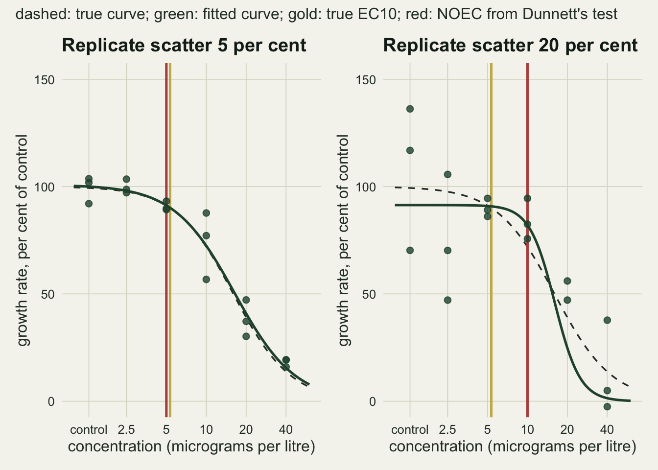
Noise and replication move the NOEC
The sweep crosses three levels of replicate scatter, 5, 10 and 20 per cent of the control mean, with three replication levels, 3, 6 and 10 flasks per concentration. Each of the nine cells gets 4000 simulated tests, so the Monte Carlo standard error of any proportion is at most 0.0079.
sd_set  <- c(5, 10, 20)
rep_set <- c(3, 6, 10)
n_rep   <- 4000
n_fit   <- 400
mc_se_max <- sqrt(0.25 / n_rep)

set.seed(6217)
cells <- expand.grid(sd_res = sd_set, n_per = rep_set)
sweep_list <- lapply(seq_len(nrow(cells)), function(i) {
  y_arr <- sim_assays(n_rep, cells$sd_res[i], cells$n_per[i], conc_grid)
  rd    <- noec_readings(y_arr, conc_grid, cells$n_per[i])
  conc_v <- rep(c(0, conc_grid), times = cells$n_per[i])
  e10 <- vapply(seq_len(n_fit), function(r)
    ec10_from_fit(fit_curve(conc_v, as.vector(y_arr[r, , ]))), numeric(3))
  list(rd = rd, e10 = e10)
})

sweep_tab <- cbind(cells, t(vapply(sweep_list, function(s) {
  ok <- !is.na(s$e10["est", ])
  e_est <- s$e10["est", ok]
  c(p_above   = mean(s$rd$low > ec10_true),
    p_down    = mean(s$rd$down > ec10_true),
    p_holm    = mean(s$rd$holm > ec10_true),
    disagree  = mean(s$rd$low != s$rd$down),
    med_noec  = median(s$rd$low),
    mean_eff  = 100 * mean(effect_at(s$rd$low)),
    fail      = mean(!ok),
    ec10_med  = exp(median(e_est)),
    ec10_q05  = exp(quantile(e_est, 0.05, names = FALSE)),
    ec10_q95  = exp(quantile(e_est, 0.95, names = FALSE)),
    ec10_up   = mean(e_est > log(ec10_true)),
    cover     = mean(s$e10["lo", ok] < log(ec10_true) &
                     s$e10["hi", ok] > log(ec10_true)),
    width     = median(exp(s$e10["hi", ok] - s$e10["lo", ok])))
}, numeric(13))))
sweep_tab$p_se <- sqrt(sweep_tab$p_above * (1 - sweep_tab$p_above) / n_rep)

cell <- function(s, n) which(sweep_tab$sd_res == s & sweep_tab$n_per == n)
c_53  <- cell(5, 3);  c_103 <- cell(10, 3); c_203 <- cell(20, 3)
c_206 <- cell(20, 6); c_2010 <- cell(20, 10); c_1010 <- cell(10, 10)
c_56  <- cell(5, 6)
max_disagree <- max(sweep_tab$disagree)
max_holm_gap <- max(abs(sweep_tab$p_holm - sweep_tab$p_above))
max_down_gap <- max(abs(sweep_tab$p_down - sweep_tab$p_above))
holm_lower   <- all(sweep_tab$p_holm <= sweep_tab$p_above)
n_above_53   <- round(sweep_tab$p_above[c_53] * n_rep)
eff_fold     <- sweep_tab$mean_eff[c_203] / sweep_tab$mean_eff[c_53]
cover_low    <- which.min(sweep_tab$cover)
cover_low_z  <- (0.95 - sweep_tab$cover[cover_low]) / sqrt(0.95 * 0.05 / n_fit)
With three flasks per concentration, the NOEC lies above the true EC10 in 0 of the 4000 tests at five per cent scatter, 18.8 per cent at ten, and 72.6 per cent at twenty (Monte Carlo standard error 0.0071 for the last). Replication pulls the figure back down but does not remove it: at twenty per cent scatter it is 43.6 per cent with six flasks and 19.1 per cent with ten.
The average true reduction in growth at the reported NOEC tells the same story on the scale a risk assessor cares about. It is 6.1 per cent for three flasks at five per cent scatter and 26.6 per cent for three flasks at twenty. The cleanest laboratory with six flasks has a median NOEC of 2.5, below the true EC10, because its test can detect the 8.9 per cent reduction at 5 micrograms per litre. The NOEC does not err in one direction: it follows the power of the test up and down, and a good test is penalised with a lower number.
Neither the reading of the LOEC rule nor the multiplicity procedure changes this. The top-down reading and the lowest-significant reading disagreed in at most 2.88 per cent of tests in any cell, and the largest difference between them in the proportion above the EC10 was 0.0178. Holm’s procedure on the same statistics gave a proportion no higher than Dunnett’s in every cell, lower by at most 0.0395. Holm starts from a Bonferroni threshold that is stricter than Dunnett’s, but it steps down: once the large effects at the top concentrations are declared, the remaining comparisons face a less strict threshold, while Dunnett’s single-step test keeps one critical value for all five. On this curve the step-down gain outweighed the stricter first step.
sweep_tab$reps <- factor(paste(sweep_tab$n_per, "flasks"),
                         levels = paste(rep_set, "flasks"))
ggplot(sweep_tab, aes(sd_res, p_above, colour = reps)) +
  geom_line(linewidth = 0.9) +
  geom_errorbar(aes(ymin = p_above - 2 * p_se, ymax = p_above + 2 * p_se),
                width = 0.6, linewidth = 0.5) +
  geom_point(size = 2.4) +
  scale_colour_manual(values = c(te_rust, te_gold, te_forest), name = NULL) +
  scale_x_continuous(breaks = sd_set) +
  scale_y_continuous(limits = c(0, 1)) +
  labs(x = "replicate scatter (per cent of control mean)",
       y = "proportion with NOEC above true EC10",
       title = "A noisier test reports a higher NOEC",
       subtitle = "bars: two Monte Carlo standard errors") +
  theme_datasheet() +
  theme(legend.position = "bottom")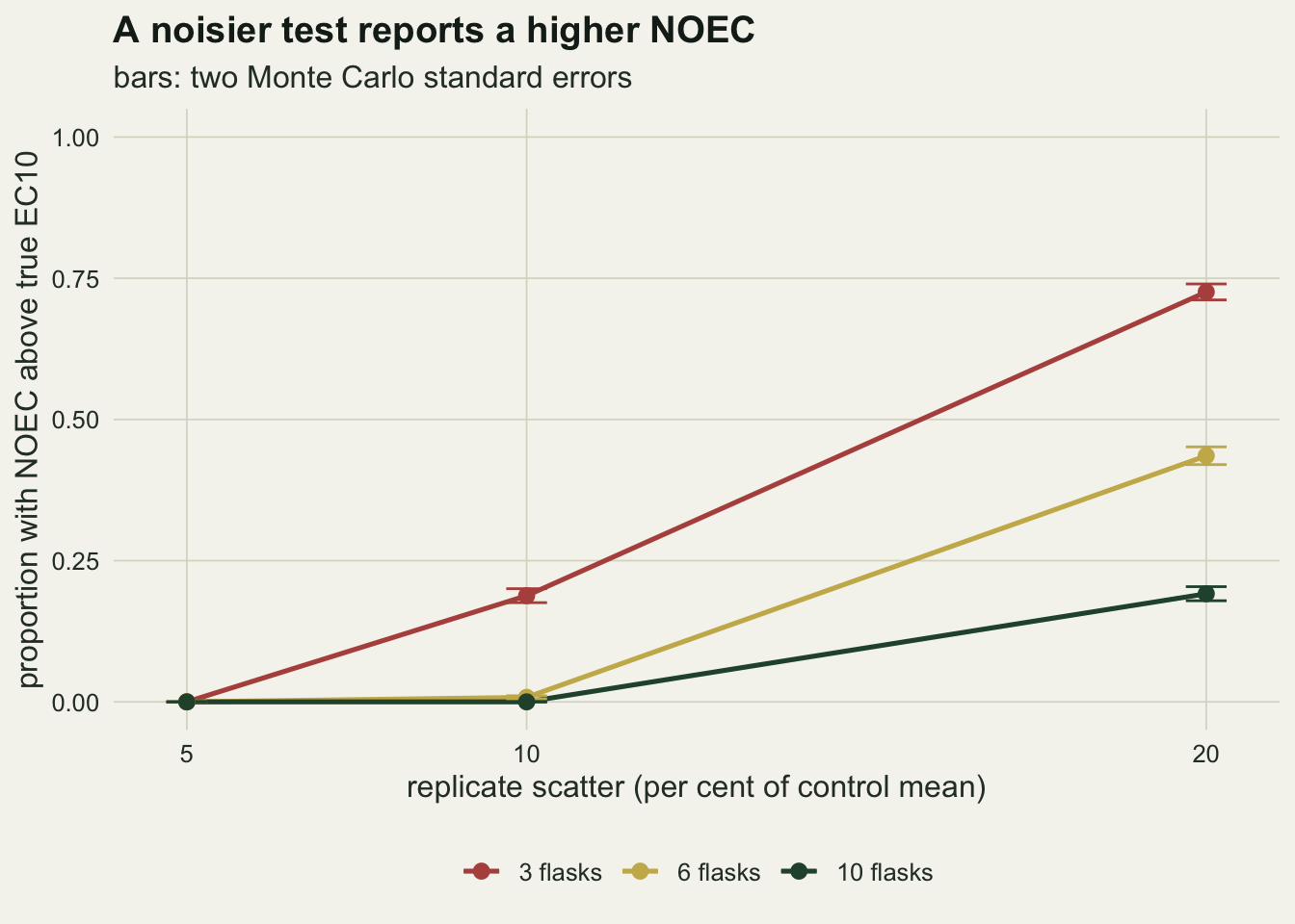
The fitted EC10 on the same tests
The first 400 tests of every cell were also analysed as a regression: the three parameter log-logistic curve fitted by nls(), the EC10 read off it as the EC50 times one ninth raised to one over the slope, and a delta method interval computed on the log scale, where the EC10 is a linear combination of the log EC50 and the reciprocal slope. A fit that fails to converge, or returns a slope of zero or less, counts as a failure and is reported as such rather than dropped silently. Starting values come from the data (control mean, the median tested concentration, a slope of 1.5), never from the truth.
fail_max   <- max(sweep_tab$fail)
fail_cell  <- sweep_tab[which.max(sweep_tab$fail), c("sd_res", "n_per")]
n_fail_tot <- round(sum(sweep_tab$fail * n_fit))
ec10_med_rng <- range(sweep_tab$ec10_med)
ec10_up_rng  <- range(sweep_tab$ec10_up)
cover_rng    <- range(sweep_tab$cover)
cover_se     <- sqrt(0.95 * 0.05 / n_fit)
width_53     <- sweep_tab$width[c_53]
width_203    <- sweep_tab$width[c_203]
width_2010   <- sweep_tab$width[c_2010]
Across the nine cells the median EC10 estimate ranges from 5.24 to 5.57 against the true 5.33, and the share of estimates above the truth ranges from 0.475 to 0.540. The noise does not push the estimate in either direction. It shows up where it belongs, in the spread: the median ratio of upper to lower interval limit is 1.70 for three flasks at five per cent scatter and 7.74 for three flasks at twenty, and ten flasks bring the second back to 2.94. Coverage of the nominal 95 per cent delta interval runs from 0.912 to 0.960, each with a Monte Carlo standard error near 0.011. The lowest value, at 20 per cent scatter with 6 flasks, is 3.4 standard errors short of 0.95, and the six cells with 10 or 20 per cent scatter average 0.935, so the delta interval runs a little narrow there; it is not a guarantee.
Fits failed in 8 of the 3600 tests in total, and the worst cell was 20 per cent scatter with 3 flasks, at 2.0 per cent. Those are tests in which a curve analysis has to say that the data do not support a curve, which is a more informative outcome than a NOEC of 40 or above.
ggplot(sweep_tab, aes(factor(sd_res), ec10_med, colour = reps)) +
  geom_hline(yintercept = ec10_true, colour = te_gold, linewidth = 0.9) +
  geom_errorbar(aes(ymin = ec10_q05, ymax = ec10_q95),
                position = position_dodge(width = 0.6), width = 0.25,
                linewidth = 0.7) +
  geom_point(position = position_dodge(width = 0.6), size = 2.6) +
  scale_colour_manual(values = c(te_rust, te_gold, te_forest), name = NULL) +
  scale_y_log10(breaks = c(2, 3, 5, 8, 12)) +
  labs(x = "replicate scatter (per cent of control mean)",
       y = "EC10 estimate (micrograms per litre)",
       title = "The EC10 widens but stays centred",
       subtitle = "gold line: true EC10; bars: 5th to 95th percentile of estimates") +
  theme_datasheet() +
  theme(legend.position = "bottom")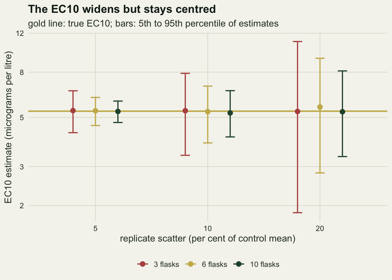
Spending the same flasks on more concentrations
A many-to-one test gains from many flasks at few concentrations, because each comparison then has more replicates behind it. A curve fit only needs enough concentrations to pin the shape. To see what the split does to each endpoint, hold the budget at 60 flasks over the same range, 2.5 to 40 micrograms per litre, and split it three ways: three concentrations a factor of four apart with 15 flasks at each level including the control, five concentrations a factor of two apart with 10, and nine concentrations a factor of the square root of two apart with 6.
budget <- list(
  "3 concentrations" = list(conc = 2.5 * 4^(0:2), n_per = 15),
  "5 concentrations" = list(conc = 2.5 * 2^(0:4), n_per = 10),
  "9 concentrations" = list(conc = 2.5 * sqrt(2)^(0:8), n_per = 6))
n_flask <- vapply(budget, function(b) (length(b$conc) + 1) * b$n_per, 0)
sd_budget <- c(10, 20)

set.seed(7384)
budget_tab <- do.call(rbind, lapply(sd_budget, function(sd_res) {
  do.call(rbind, lapply(names(budget), function(nm) {
    conc  <- budget[[nm]]$conc
    n_per <- budget[[nm]]$n_per
    y_arr <- sim_assays(n_rep, sd_res, n_per, conc)
    noec  <- noec_readings(y_arr, conc, n_per)$low
    conc_v <- rep(c(0, conc), times = n_per)
    e10 <- vapply(seq_len(n_fit), function(r)
      ec10_from_fit(fit_curve(conc_v, as.vector(y_arr[r, , ])))[["est"]], 0)
    ok <- !is.na(e10)
    p_big <- mean(effect_at(noec) > 0.10)
    data.frame(design = nm, sd_res = sd_res,
               p_big = p_big, p_big_se = sqrt(p_big * (1 - p_big) / n_rep),
               mean_eff = 100 * mean(effect_at(noec)),
               fail = mean(!ok),
               ratio90 = exp(quantile(e10[ok], 0.95, names = FALSE) -
                             quantile(e10[ok], 0.05, names = FALSE)))
  }))
}))
bt <- function(s, d) which(budget_tab$sd_res == s & budget_tab$design == d)
b_3_20 <- bt(20, "3 concentrations"); b_5_20 <- bt(20, "5 concentrations")
b_9_20 <- bt(20, "9 concentrations"); b_3_10 <- bt(10, "3 concentrations")
b_9_10 <- bt(10, "9 concentrations"); b_5_10 <- bt(10, "5 concentrations")
fail_budget <- max(budget_tab$fail)
eff_coarse  <- 100 * effect_at(2.5 * 4^(0:2))
All three designs use 60 flasks. At twenty per cent scatter the true reduction at the NOEC exceeds ten per cent in 3.7 per cent of tests with three concentrations, 20.1 per cent with five and 81.5 per cent with nine. At ten per cent scatter the three figures are 0.0, 0.0 and 34.2 per cent. The fitted EC10 also spreads a little more as the flasks are thinned, but on a different scale of change: the ratio of the 95th to the 5th percentile of the estimates at twenty per cent scatter is 2.14, 2.57 and 2.57 for the three designs, and fits failed in at most 0.5 per cent of tests in any of the six settings.
The coarse design looks best for the NOEC, and the reason is not a virtue. With concentrations at 2.5, 10 and 40 the true reductions are 2.4, 28.1 and 86.2 per cent, so there is no tested concentration between a negligible effect and a large one. Fifteen flasks detect the jump, the NOEC usually lands on the lowest concentration, and the endpoint says nothing about where between 2.5 and 10 the effect begins. The NOEC can only be a concentration that was tested, so the grid decides which numbers it is allowed to take, and a finer grid gives a noisy test more chances to stop late.
budget_tab$scatter <- factor(paste(budget_tab$sd_res, "per cent scatter"),
                             levels = paste(sd_budget, "per cent scatter"))
p_left <- ggplot(budget_tab, aes(design, p_big, colour = scatter,
                                 group = scatter)) +
  geom_line(linewidth = 0.9) +
  geom_errorbar(aes(ymin = p_big - 2 * p_big_se, ymax = p_big + 2 * p_big_se),
                width = 0.12, linewidth = 0.5) +
  geom_point(size = 2.4) +
  scale_colour_manual(values = c(te_forest, te_rust), name = NULL) +
  scale_y_continuous(limits = c(0, 1)) +
  labs(x = NULL, y = "share with effect at NOEC over 10%",
       title = "NOEC") +
  theme_datasheet() +
  theme(legend.position = "none")
p_right <- ggplot(budget_tab, aes(design, ratio90, colour = scatter,
                                  group = scatter)) +
  geom_line(linewidth = 0.9) +
  geom_point(size = 2.4) +
  scale_colour_manual(values = c(te_forest, te_rust), name = NULL) +
  scale_y_continuous(limits = c(1, NA)) +
  labs(x = NULL, y = "95th over 5th percentile of EC10",
       title = "Fitted EC10") +
  theme_datasheet() +
  theme(legend.position = "none")
(p_left | p_right) +
  plot_annotation(subtitle = paste("60 flasks over 2.5 to 40 micrograms per litre;",
                                   "green: 10 per cent scatter, red: 20 per cent"),
                  theme = theme_datasheet()) &
  theme(axis.text.x = element_text(angle = 20, hjust = 1))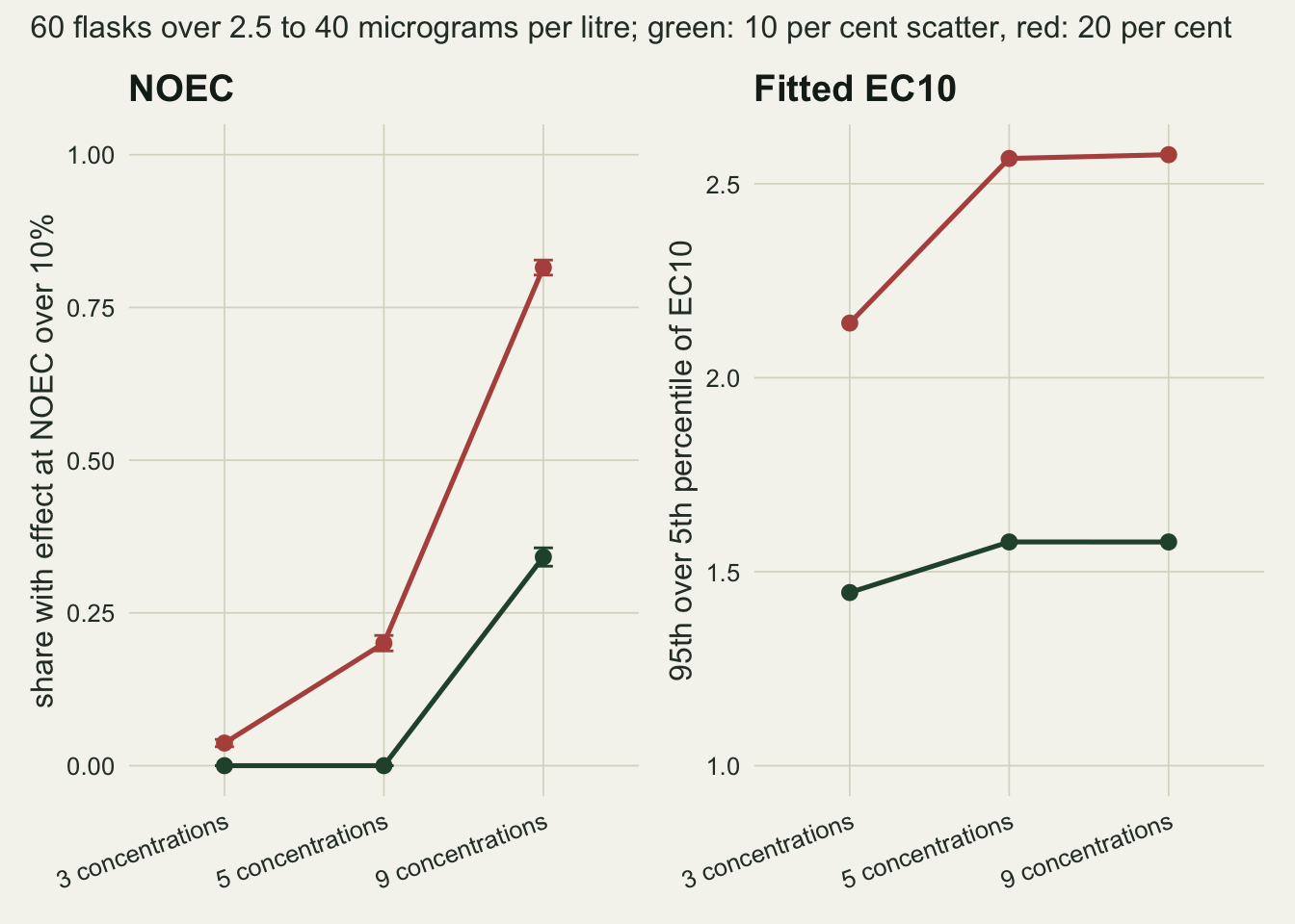
What to report
If a NOEC has to be reported because a guideline asks for it, report the power that produced it. The minimum detectable difference of the test, as a percentage of the control mean, turns a NOEC into a statement that can be checked, because two equal NOECs from tests with very different detectable differences are not the same finding. Crane and Newman asked how large an effect a NOEC from a standard design can hide, and the sweep above shows why the answer depends on the design: for one true curve, the average true reduction at the reported NOEC was 4.3 times larger with three flasks at twenty per cent scatter than with three flasks at five.
Report the replicate scatter as the coefficient of variation of the control, the number of replicates and the concentration spacing next to the NOEC. Those three quantities decide the endpoint as much as the substance does.
Where the data allow it, report a fitted ECx with its interval as the primary endpoint and the NOEC as a secondary one. The EC10 from the same tests stayed centred on the truth at every level of scatter and replication measured here; what noise did to it was widen its interval, which is the honest direction for a worse experiment to move a number. Say which model was fitted, how the interval was computed, and how many fits failed.
Name the multiplicity procedure and the reading of the LOEC rule. Here the choice between Dunnett and Holm moved the proportions by a few percentage points and the choice between the lowest-significant and top-down readings by less, without changing their order, but a reader cannot know that for a different design unless it is stated.
Honest limits
The response is Gaussian with constant variance on the percentage scale, and the curve has no hormesis, no threshold and no control drift. Real reproduction counts are overdispersed, growth rates can be heteroscedastic, and a biphasic response breaks both the monotone-test logic and the three parameter curve. None of those cases is simulated, and the fitted EC10 would not stay centred under a misspecified curve the way it does here, where the fitted model is the true one.
Williams’ test, which assumes a monotone decrease and pools neighbouring means under that order, is the other standard route to a NOEC for a continuous response and has more power than Dunnett’s test when the order holds. It would be expected to lower every proportion in the sweep, but not to change the direction, because it is still a significance test whose power falls with scatter. That is an argument rather than a measurement, and the numbers here are for Dunnett’s test and Holm’s procedure only.
The NOEC is compared with the EC10 throughout. A regulator who compares a NOEC with an EC20, or who treats a ten per cent reduction as negligible for this endpoint, would draw the threshold elsewhere, and every proportion above would change with it. The comparison is between an endpoint and a curve quantity, and the choice of ten per cent is conventional rather than biological.
The EC10 interval is the delta method on the log scale, with t quantiles on the residual degrees of freedom. Confidence intervals for effective doses shows that profile and Fieller intervals behave differently in the tail of a binomial curve, and nothing here checks whether that ranking carries over to a continuous response. The coverage figures are for 400 fits per cell, which resolves departures of a few percentage points and no finer.
The grid, the curve and the scatter levels are one choice each. The proportions in the sweep figure depend on where the true EC10 sits between two tested concentrations, as the fixed-budget section shows directly, and they should be read as the size of the effect for this grid rather than as a rate that transfers to other tests.
References
Dunnett CW 1955 Journal of the American Statistical Association 50(272):1096-1121 (10.1080/01621459.1955.10501294)
Williams DA 1971 Biometrics 27(1):103-117 (10.2307/2528930)
Laskowski R 1995 Oikos 73(1):140-144 (10.2307/3545738)
Crane M, Newman MC 2000 Environmental Toxicology and Chemistry 19(2):516-519 (10.1002/etc.5620190234)
Jager T 2012 Environmental Toxicology and Chemistry 31(2):228-229 (10.1002/etc.746)