---
title: "Observed power tells you nothing"
description: "Power computed from the effect you observed is a one-to-one function of the p value, so it cannot say whether a non-significant study was underpowered."
date: "2026-08-12 15:00"
date-modified: "2026-10-15"
categories: [R, hypothesis testing, study design, statistics, ecology tutorial]
image: thumbnail.png
image-alt: "A scatter of observed power against the p value in which every point from three different true effect sizes falls on one smooth descending curve."
---
*Corrected 15 October 2026: the post said two one-sided tests give a verdict where a non-significant test gives none; it now says they can give a verdict of equivalence, which a non-significant test cannot, and that with data as imprecise as the small study's they give none either.*
*Corrected 7 October 2026: the post said the small study in the two-study comparison happens to land half a standard deviation from zero, and the first figure's text description said the null studies gather at the high p end; it now says that distance is set by choosing the studies for their p value, and that the null studies spread along the whole curve.*
A referee writes: the difference between your treatments was not significant, so please report the power of your test. The author obliges, plugs the observed difference and the observed variance into a power calculation, and reports something like 0.19. The referee reads that as confirmation that the study was too small.
It is not confirmation of anything. Power computed from the effect you observed is a rearrangement of the p value you already reported, and it contains no information the p value did not.
## The claim, and how to check it
The claim is strong enough to be tested directly rather than argued. Simulate a large number of two-sample comparisons, at several true effect sizes so the data sets differ in more than noise, and compute both numbers for each one.
```{r setup}
#| message: false
#| warning: false
library(ggplot2)

te_paper  <- "#f5f4ee"
te_ink    <- "#16241d"
te_body   <- "#2c3a31"
te_forest <- "#275139"
te_rust   <- "#b5534e"
te_gold   <- "#c9b458"
te_line   <- "#dad9ca"

theme_datasheet <- function() {
  theme_minimal(base_size = 12) +
    theme(plot.background  = element_rect(fill = te_paper, colour = NA),
          panel.background = element_rect(fill = te_paper, colour = NA),
          panel.grid.major = element_line(colour = te_line, linewidth = 0.3),
          panel.grid.minor = element_blank(),
          text             = element_text(colour = te_body),
          plot.title       = element_text(colour = te_ink, face = "bold"),
          axis.text        = element_text(colour = te_body))
}

# power at the effect size and variance the study happened to observe
observed_power <- function(x, y, alpha = 0.05) {
  n  <- length(x)
  sp <- sqrt(((n - 1) * var(x) + (n - 1) * var(y)) / (2 * n - 2))
  power.t.test(n = n, delta = abs(mean(x) - mean(y)), sd = sp,
               sig.level = alpha)$power
}

one_study <- function(n, true_diff) {
  x <- rnorm(n)
  y <- rnorm(n, true_diff)
  c(p = t.test(x, y, var.equal = TRUE)$p.value,
    power = observed_power(x, y),
    n = n, true_diff = true_diff)
}

set.seed(20260812)
sims <- do.call(rbind, lapply(c(0, 0.3, 0.6), function(d)
  as.data.frame(t(replicate(400, one_study(20, d))))))
nrow(sims)
```
```{r rho}
c(spearman = cor(sims$p, sims$power, method = "spearman"))
```
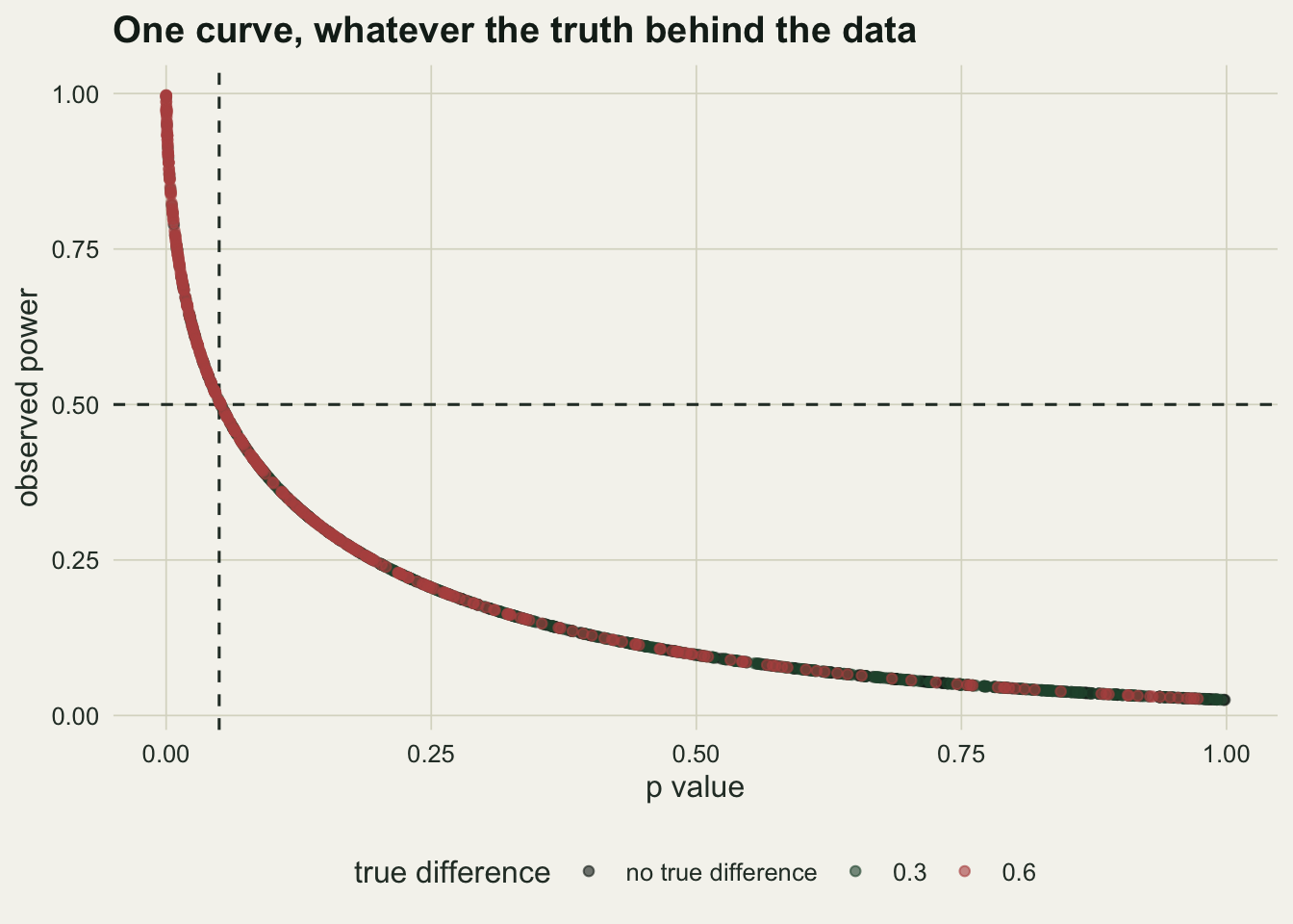
A rank correlation of `r sprintf("%.0f", cor(sims$p, sims$power, method = "spearman"))` across `r nrow(sims)` studies from three different truths. Not close to minus one: minus one. Sort the studies by p value and you have sorted them by observed power, in reverse, with no ties broken differently and nothing left over.
That is what it means for one number to be a function of another. Reporting both is reporting the same thing twice.
```{r fig-curve}
#| fig-cap: "Observed power against the p value for 1200 simulated two-sample tests at three true effect sizes."
#| fig-alt: "A scatter plot with the p value on the x axis and observed power on the y axis. The 1200 points form a single curve one point wide, falling steeply from the top left corner and flattening towards the bottom right. Points from all three true effect sizes lie on that same curve and overlap; colour separates them only in where they sit along it, the largest effect gathered near the low p end and the null spread along the whole length of it. Dashed lines cross at a p value of 0.05 and an observed power of one half."
sims$truth <- factor(sims$true_diff,
                     labels = c("no true difference", "0.3", "0.6"))

ggplot(sims, aes(x = p, y = power)) +
  geom_hline(yintercept = 0.5, linetype = "dashed", colour = te_body) +
  geom_vline(xintercept = 0.05, linetype = "dashed", colour = te_body) +
  geom_point(aes(colour = truth), size = 1.5, alpha = 0.6) +
  scale_colour_manual(values = c(te_ink, te_forest, te_rust)) +
  labs(x = "p value", y = "observed power", colour = "true difference",
       title = "One curve, whatever the truth behind the data") +
  theme_datasheet() +
  theme(legend.position = "bottom")
```
## The mapping, in numbers
Because it is a function, it can be tabulated. The interesting entry is at the conventional threshold.
```{r at-threshold}
near <- abs(sims$p - 0.05) < 0.005
round(c(studies = sum(near),
        mean_observed_power = mean(sims$power[near]),
        lowest  = min(sims$power[near]),
        highest = max(sims$power[near])), 3)
```
A study that lands exactly on p equal to 0.05 has observed power of about a half. Every time. And it is not an artefact of this sample size.
```{r across-n}
set.seed(4)
by_n <- do.call(rbind, lapply(c(10, 20, 60), function(n)
  as.data.frame(t(replicate(400, one_study(n, 0.4))))))
tab <- do.call(rbind, lapply(c(10, 20, 60), function(n) {
  s <- by_n[by_n$n == n & abs(by_n$p - 0.05) < 0.006, ]
  data.frame(n = n, studies = nrow(s), power_at_p_05 = mean(s$power))
}))
round(tab, 4)
pooled_rho <- cor(by_n$p, by_n$power, method = "spearman")
round(pooled_rho, 5)
```
Ten per group or sixty per group, the answer at p equal to 0.05 is the same half. The whole curve shifts a little with sample size, which is why the rank correlation over the pooled set is `r sprintf("%.4f", pooled_rho)` rather than exactly minus one, but over a sixfold change in sample size the value at the threshold moves by about one part in a hundred, and no reader is going to learn anything from that.
The other end is worth stating too, because it is where the referee's question lives.
```{r high-p}
round(c(largest_observed_power_when_p_above_half =
          max(sims$power[sims$p > 0.5])), 3)
```
Of the studies with a p value above 0.5, not one had observed power above `r sprintf("%.2f", max(sims$power[sims$p > 0.5]))`. And because the curve is monotone, the ceiling for a non-significant result is the value at the threshold: no study with p above 0.05 can report observed power above about a half, and the further above 0.05 the p value goes the lower the ceiling drops. That bound is arithmetic, not something discovered in the data, so a value under it cannot be evidence that the study was underpowered. It would have come out under it whether the study was tiny or enormous.
## The question the referee meant to ask
Behind the request there is a real question, and it is a good one: does this non-significant result rule out effects large enough to matter, or is it simply uninformative? That question has an answer. Observed power is not it, and the interval already printed in the output is.
Here are two studies with the same p value.
```{r two-studies}
find_study <- function(n, target_p = 0.30, tol = 0.01) {
  repeat {
    x <- rnorm(n)
    y <- rnorm(n)
    tt <- t.test(x, y, var.equal = TRUE)
    if (abs(tt$p.value - target_p) < tol) return(list(x = x, y = y, tt = tt))
  }
}
set.seed(3)
small <- find_study(12)
large <- find_study(400)

two <- data.frame(
  study = c("12 per group", "400 per group"),
  p     = c(small$tt$p.value, large$tt$p.value),
  diff  = c(diff(rev(small$tt$estimate)), diff(rev(large$tt$estimate))),
  lower = c(small$tt$conf.int[1], large$tt$conf.int[1]),
  upper = c(small$tt$conf.int[2], large$tt$conf.int[2]),
  obs_power = c(observed_power(small$x, small$y),
                observed_power(large$x, large$y)))
round(two[, -1], 3)
```
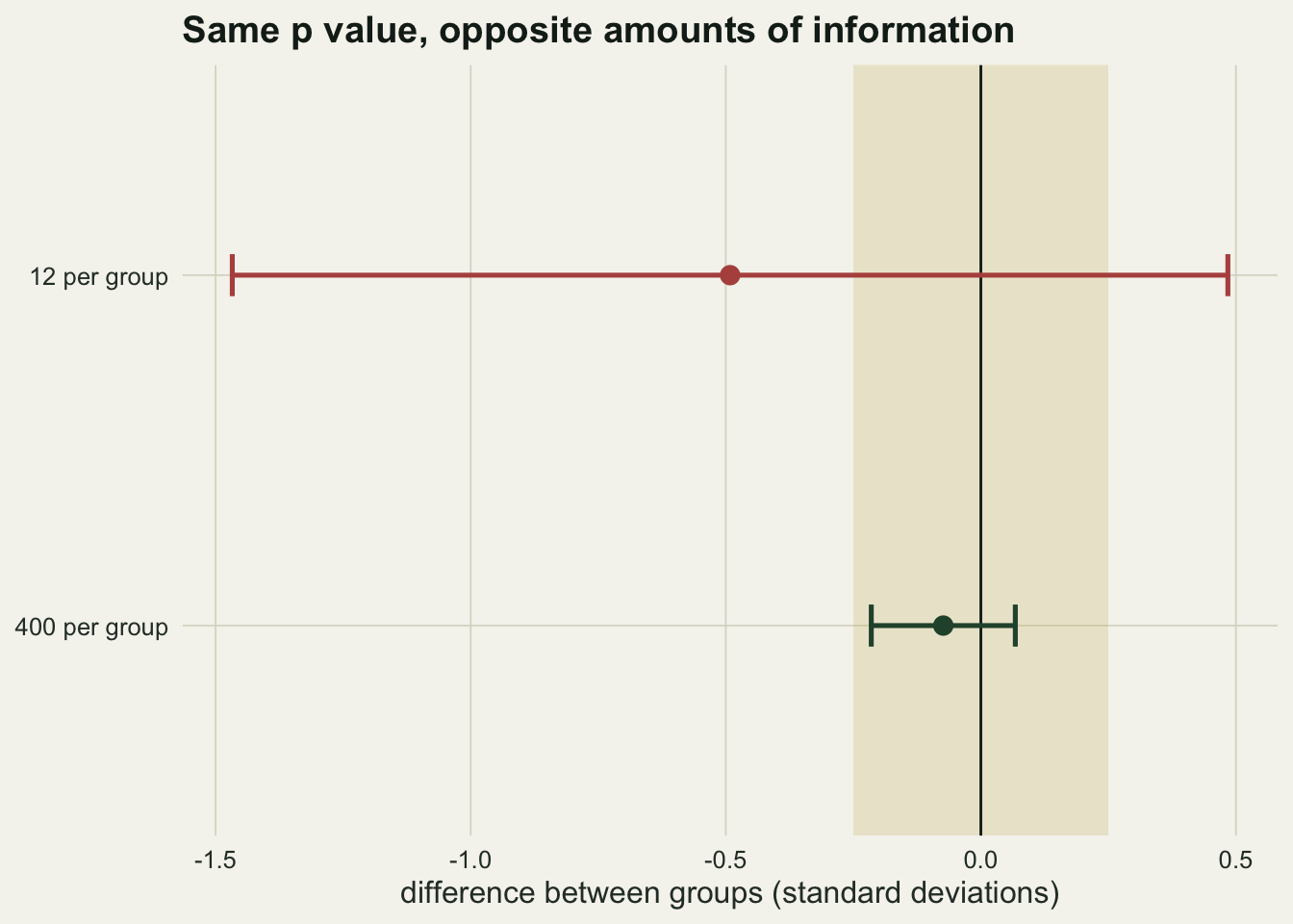
Both are non-significant, at `r sprintf("%.3f", two$p[1])` and `r sprintf("%.3f", two$p[2])`. Both have observed power near `r sprintf("%.2f", mean(two$obs_power))`. On the evidence the referee asked for, they are the same study.
They are not the same study. The interval from the small one runs from `r sprintf("%.2f", two$lower[1])` to `r sprintf("%.2f", two$upper[1])` standard deviations, which is compatible with a difference large enough to change management. The interval from the large one runs from `r sprintf("%.2f", two$lower[2])` to `r sprintf("%.2f", two$upper[2])`, which rules out anything that would. One of these results is uninformative and the other is an informative null, and the p value cannot tell them apart because it was never trying to.
```{r fig-intervals}
#| fig-cap: "Confidence intervals for the two studies above, both non-significant with almost the same p value, against a band of differences small enough to ignore."
#| fig-alt: "Two horizontal intervals on a common axis of difference in standard deviations, with a pale shaded band from minus a quarter to plus a quarter marking negligible differences and a solid line at zero. The upper interval, from the study with twelve per group, spans most of the axis and runs out past both edges of the band, far past the left one. The lower interval, from four hundred per group, is short and lies entirely inside the band."
two$study <- factor(two$study, levels = rev(two$study))

ggplot(two, aes(y = study)) +
  annotate("rect", xmin = -0.25, xmax = 0.25, ymin = -Inf, ymax = Inf,
           fill = te_gold, alpha = 0.22) +
  geom_vline(xintercept = 0, colour = te_ink, linewidth = 0.5) +
  geom_errorbar(aes(xmin = lower, xmax = upper, colour = study),
                width = 0.12, linewidth = 0.9) +
  geom_point(aes(x = diff, colour = study), size = 3) +
  scale_colour_manual(values = c(te_forest, te_rust)) +
  labs(x = "difference between groups (standard deviations)", y = NULL,
       title = "Same p value, opposite amounts of information") +
  theme_datasheet() +
  theme(legend.position = "none")
```
The shaded band is the part that has to come from the biology rather than the data: a range of differences small enough that the study would treat them as no effect. Draw it and the two studies separate immediately. That comparison, made formal, is an equivalence test, and it is the procedure that answers the referee.
## What to report instead
If the question is whether the design was adequate, the answer is a power calculation done at an effect size chosen for its scientific meaning, not at the one the data happened to produce. That number is a property of the design and it does not change when the data come in, which is exactly why it is worth reporting.
For what this particular study established, the estimate and its interval are the report, together with a sentence naming the largest effect the data are compatible with. That sentence does more work than any power figure.
If the question is whether the effect is negligible, state the bound in advance and test against it. Two one-sided tests can give a verdict of equivalence, which a non-significant test never can; with data as imprecise as the small study's, they too end without one.
None of the three needs the observed effect size fed back into a power formula, and there is no fourth question for which that calculation is the right answer.
## Honest limits
The demonstration uses a two-sample t test, where the algebra is cleanest: for a fixed sample size, observed power is a strictly increasing function of the absolute test statistic and the p value a strictly decreasing function of the same statistic, so the relationship between them is exact. In more complicated models with several parameters, nuisance terms, or a variance component estimated from the same data, the correspondence loosens. It loosens; it does not become informative.
Retrospective power calculated at an externally specified effect size is a different quantity and a legitimate one. The objection here is to power calculated at the observed effect, which is the version that reviewers usually mean and that software makes easiest to produce.
The two-study comparison draws both data sets under no true difference, so neither estimate is centred on a real effect: the small study lands about half a standard deviation from zero because, with twelve per group, that is roughly how far from zero an estimate has to sit to give that p value. With a real effect the widths behave the same way and the centres do not, and the interval is still the thing to read.
Finally, the argument here is about interpretation, not about anyone's competence. The calculation is intuitive, it is one line in R, and the reason it keeps appearing is that the question it seems to answer is a genuinely important one.
## References
Hoenig JM, Heisey DM 2001 The American Statistician 55(1):19-24 (10.1198/000313001300339897)
Levine M, Ensom MHH 2001 Pharmacotherapy 21(4):405-409 (10.1592/phco.21.5.405.34503)
Greenland S, Senn SJ, Rothman KJ, Carlin JB, Poole C, Goodman SN, Altman DG 2016 European Journal of Epidemiology 31(4):337-350 (10.1007/s10654-016-0149-3)
## Related tutorials
- [Power analysis by simulation](../power-analysis-by-simulation/)
- [Testing for no effect: equivalence tests in R](../testing-for-no-effect/)
- [What a p-value tells you, and what it does not](../what-a-p-value-tells-you/)
- [Comparing significance is not a test](../comparing-significance-is-not-a-test/)