library(ggplot2)

te_paper  <- "#f5f4ee"
te_ink    <- "#16241d"
te_body   <- "#2c3a31"
te_forest <- "#275139"
te_rust   <- "#b5534e"
te_gold   <- "#c9b458"
te_line   <- "#dad9ca"

theme_datasheet <- function() {
  theme_minimal(base_size = 12) +
    theme(plot.background  = element_rect(fill = te_paper, colour = NA),
          panel.background = element_rect(fill = te_paper, colour = NA),
          panel.grid.major = element_line(colour = te_line, linewidth = 0.3),
          panel.grid.minor = element_blank(),
          text             = element_text(colour = te_body),
          plot.title       = element_text(colour = te_ink, face = "bold"),
          plot.subtitle    = element_text(colour = te_body),
          axis.text        = element_text(colour = te_body))
}Home vs away and local vs foreign in transplants
R
local adaptation
experimental design
interactions
simulation
ecology tutorial
Two criteria for local adaptation in a reciprocal transplant, the main effect each mistakes for adaptation, and why populations, not plants, are the replicate.
A perennial herb grows on two kinds of ground a few kilometres apart: deep loam in a valley meadow and a thin serpentine outcrop on the ridge above it. Seed is collected from both populations, raised to seedlings, and planted back out in a reciprocal transplant, twenty plants of each population at each site. At the end of the season every plant’s seed output is counted. The loam plants set far more seed in the meadow than on the ridge, the difference is significant, and the result is written up as local adaptation of the loam population to its home soil.
The serpentine plants were planted on the same two sites, and they also set more seed in the meadow than on the ridge. The meadow is simply the better place to be a plant. So the loam population’s home advantage is the same thing the serpentine population shows as a home disadvantage, and neither number, on its own, says anything about adaptation.
Kawecki and Ebert 2004 set out two criteria for reading a transplant. The home vs away criterion asks, for each population, whether it does better in its own habitat than in the other habitats. The local vs foreign criterion asks, for each habitat, whether the local population does better than the populations brought in from elsewhere. They regard the local vs foreign criterion as the diagnostic one, and they point out that home vs away confounds divergent selection with intrinsic differences in habitat quality. They also give the pattern a single summary: fitness should be systematically higher in the sympatric combinations, where a population is tested in its habitat of origin, than in the allopatric ones. Blanquart and colleagues 2013 recommend testing local adaptation with exactly that sympatric vs allopatric contrast, in a linear model that also carries habitat and population quality effects. A survey of published transplants by Hereford 2009 put the overall frequency of local adaptation at 0.71, scoring it as a native population doing better than foreign ones at its home site; that is a local vs foreign contrast, one site at a time, and below it turns out to be the contrast a difference in population quality inflates.
This post measures what each criterion does in a two by two transplant when there is no local adaptation at all, only a better site or a better population, and then how much each one detects when local adaptation is real. The criteria are applied in two ways, the strict form Kawecki and Ebert define (the pattern in every population, or in every habitat) and a looser reading that takes one population, or one site, at a time and declares adaptation when at least one of them shows the pattern. The last simulation asks what the interaction test itself needs: what counts as a replicate when the claim is adaptation to a habitat.
Three posts sit next to this one. Comparing significance is not a test is about two separate verdicts compared by eye in place of an interaction test; here each criterion is a proper contrast with its own test, and the problem is that it is a contrast for a different question. Term order in unbalanced factorial ANOVA is about which hypothesis a sequential table tests when cells are unequal; the transplant below is balanced, and the test it ends up recommending is the interaction, which comes last in either order. Qst against Fst looks for divergent selection from a common garden and marker data; a reciprocal transplant is the field route to the same question.
Four contrasts built from two numbers
The response is log seed output per plant, with residual standard deviation one on that scale. Each of the four cell means is the sum of a population effect, a site effect and a sympatric effect, the last one being the local adaptation. Every effect is split symmetrically, half added and half subtracted, so each parameter is exactly the difference it names.
n_cell    <- 20          # plants per population and site
sigma_res <- 1           # residual sd of log seed output
alpha_lev <- 0.05        # one sided: adaptation is a directional claim
df_res    <- 4 * (n_cell - 1)
crit      <- qt(1 - alpha_lev, df_res)
halve     <- log(2)      # a site or population that sets half the seed

# cells: L = loam population, S = serpentine population; site M = meadow, R = ridge
cell_means <- function(site_eff, pop_eff, sym_eff) {
  c(L_M =  pop_eff / 2 + site_eff / 2 + sym_eff / 2,
    L_R =  pop_eff / 2 - site_eff / 2 - sym_eff / 2,
    S_M = -pop_eff / 2 + site_eff / 2 - sym_eff / 2,
    S_R = -pop_eff / 2 - site_eff / 2 + sym_eff / 2)
}
Written out, the two home vs away contrasts are the loam population in the meadow minus the loam population on the ridge, and the serpentine population on the ridge minus the serpentine population in the meadow. The two local vs foreign contrasts are the loam population minus the serpentine population in the meadow, and the serpentine population minus the loam population on the ridge. Substituting the cell means gives the whole post in four lines. The loam population’s home advantage has expectation equal to the local adaptation plus the site effect; the serpentine population’s has the local adaptation minus the site effect. The local vs foreign contrast in the meadow has the local adaptation plus the population effect, and on the ridge the local adaptation minus the population effect. Half the sum of either pair is the sympatric vs allopatric contrast, and it contains neither main effect. Blanquart and colleagues define their home vs away and local vs foreign measures as averages over populations and over sites, and show that in expectation both averages equal the sympatric vs allopatric contrast; in a two by two design that is the algebra just written. The trouble lives in the individual contrasts, one population or one site at a time.
So each criterion is immune to one main effect and carries the other. Home vs away never sees a difference in population quality, because it compares a population with itself; local vs foreign never sees a difference in site quality, because it compares populations on the same ground. And requiring the pattern in both populations, or in both sites, is the same as requiring the local adaptation to exceed the relevant main effect in size.
In a balanced design all of this depends on the data only through the four cell means and the residual sum of squares, so a simulation can draw those directly. That is a shortcut to check against lm(), not to assume.
contrasts_from <- function(m, s2) {
  se_one <- sqrt(s2 * 2 / n_cell)            # one cell mean minus another
  se_sa  <- sqrt(s2 / n_cell)                # half the sum of two such differences
  cbind(hva_L = (m[, "L_M"] - m[, "L_R"]) / se_one,
        hva_S = (m[, "S_R"] - m[, "S_M"]) / se_one,
        lvf_M = (m[, "L_M"] - m[, "S_M"]) / se_one,
        lvf_R = (m[, "S_R"] - m[, "L_R"]) / se_one,
        sa    = (m[, "L_M"] + m[, "S_R"] - m[, "L_R"] - m[, "S_M"]) / 2 / se_sa)
}
sim_fast <- function(n_rep, site_eff, pop_eff, sym_eff) {
  mu <- cell_means(site_eff, pop_eff, sym_eff)
  m <- matrix(rnorm(4 * n_rep, rep(mu, each = n_rep), sigma_res / sqrt(n_cell)),
              ncol = 4, dimnames = list(NULL, names(mu)))
  s2 <- sigma_res^2 * rchisq(n_rep, df_res) / df_res
  contrasts_from(m, s2)
}
rules <- function(tt) {
  flag <- tt > crit
  c(hva_one  = mean(flag[, "hva_L"] | flag[, "hva_S"]),
    hva_each = mean(flag[, "hva_L"] & flag[, "hva_S"]),
    lvf_one  = mean(flag[, "lvf_M"] | flag[, "lvf_R"]),
    lvf_each = mean(flag[, "lvf_M"] & flag[, "lvf_R"]),
    hva_L    = mean(flag[, "hva_L"]), hva_S = mean(flag[, "hva_S"]),
    lvf_M    = mean(flag[, "lvf_M"]), lvf_R = mean(flag[, "lvf_R"]),
    sa       = mean(flag[, "sa"]))
}
make_plants <- function(site_eff, pop_eff, sym_eff) {
  plants <- expand.grid(plant = seq_len(n_cell), pop = c("loam", "serpentine"),
                        site = c("meadow", "ridge"))
  key <- paste0(ifelse(plants$pop == "loam", "L", "S"), "_",
                ifelse(plants$site == "meadow", "M", "R"))
  plants$log_seed <- cell_means(site_eff, pop_eff, sym_eff)[key] +
                     rnorm(nrow(plants), 0, sigma_res)
  plants
}
A poorer site manufactures a home advantage
The first scenario has no local adaptation and no difference between the populations. The ridge is a poorer site, and a plant of either population sets half as many seeds there as in the meadow, which on the log scale is a site effect of 0.693. The datasets below are drawn from that process until the first one in which the loam population passes the home vs away test; it is not a rare draw, as the next section measures.
set.seed(2004)
n_tried <- 0
repeat {
  n_tried <- n_tried + 1
  plants <- make_plants(halve, 0, 0)
  fit_cells <- lm(log_seed ~ 0 + pop:site, data = plants)
  cm <- coef(fit_cells)
  m_obs <- matrix(cm[c("poploam:sitemeadow", "poploam:siteridge",
                       "popserpentine:sitemeadow", "popserpentine:siteridge")],
                  nrow = 1, dimnames = list(NULL, c("L_M", "L_R", "S_M", "S_R")))
  s2_obs <- deviance(fit_cells) / df.residual(fit_cells)
  t_obs <- contrasts_from(m_obs, s2_obs)
  if (t_obs[, "hva_L"] > crit) break
}
p_one <- pt(t_obs, df_res, lower.tail = FALSE)
diff_obs <- t_obs * sqrt(s2_obs * c(2, 2, 2, 2, 1) / n_cell)

plants$pop_s  <- plants$pop;  contrasts(plants$pop_s)  <- contr.sum(2)
plants$site_s <- plants$site; contrasts(plants$site_s) <- contr.sum(2)
fit_sum <- lm(log_seed ~ pop_s * site_s, data = plants)
t_int   <- summary(fit_sum)$coefficients["pop_s1:site_s1", "t value"]
aov_tab <- anova(fit_sum)
f_int   <- aov_tab["pop_s:site_s", "F value"]; p_int_two <- aov_tab["pop_s:site_s", "Pr(>F)"]
id_gap  <- max(abs(c(t_int - t_obs[, "sa"], f_int - t_obs[, "sa"]^2)))
seed_ratio_L <- exp(diff_obs[, "hva_L"]); seed_ratio_S <- exp(-diff_obs[, "hva_S"])
round(rbind(difference = diff_obs[1, ], t = t_obs[1, ], one_sided_p = p_one[1, ]), 3)
hva_L hva_S lvf_M lvf_R sa
difference 0.705 -0.541 0.113 0.050 0.082
t 2.229 -1.711 0.358 0.159 0.366
one_sided_p 0.014 0.954 0.360 0.437 0.358It took 2 draws. In this dataset the loam plants set 2.02 times as much seed in the meadow as on the ridge, a one sided p value of 0.014 for home against away. The serpentine plants, on the same two sites, set 1.72 times as much in the meadow as at home on the ridge, so their home vs away contrast is -0.541 on the log scale with a one sided p value of 0.954. The local vs foreign contrasts are 0.113 in the meadow and 0.050 on the ridge, with one sided p values of 0.360 and 0.437. The sympatric vs allopatric contrast is 0.082, with a one sided p value of 0.358.
That last contrast is the population by site interaction, and nothing special is needed to fit it. With sum to zero coding for both factors, the interaction coefficient of lm() is half the sympatric vs allopatric contrast, and its t value matches the hand computation to 2.4e-15; the interaction F in the analysis of variance table is the square of the same t, 0.134, and its p value of 0.715 is the two sided version. The one sided p value is the two sided one halved when the contrast points in the sympatric direction, and one minus half of it otherwise.
cell_df <- data.frame(
  pop  = factor(c("loam", "loam", "serpentine", "serpentine")),
  site = factor(c("meadow", "ridge", "meadow", "ridge")),
  est  = as.vector(m_obs[1, c("L_M", "L_R", "S_M", "S_R")]))
cell_df$half <- qt(0.975, df_res) * sqrt(s2_obs / n_cell)
cell_df$home <- ifelse((cell_df$pop == "loam") == (cell_df$site == "meadow"),
                       "at home", "away")
ggplot(cell_df, aes(site, est, colour = pop, group = pop)) +
  geom_jitter(data = plants, aes(site, log_seed, colour = pop), inherit.aes = FALSE,
              width = 0.12, height = 0, alpha = 0.25, size = 1.2) +
  geom_line(linewidth = 0.9, position = position_dodge(width = 0.25)) +
  geom_errorbar(aes(ymin = est - half, ymax = est + half), width = 0.12,
                linewidth = 0.6, position = position_dodge(width = 0.25)) +
  geom_point(aes(shape = home), size = 3.2, fill = te_paper, stroke = 1.1,
             position = position_dodge(width = 0.25)) +
  scale_colour_manual(values = c(loam = te_forest, serpentine = te_rust),
                      name = "population") +
  scale_shape_manual(values = c("at home" = 16, "away" = 21), name = NULL) +
  labs(x = "transplant site", y = "log seed output per plant",
       title = "Both populations do better in the meadow",
       subtitle = "filled points: plants at home, open points: plants away") +
  theme_datasheet() + theme(legend.position = "bottom")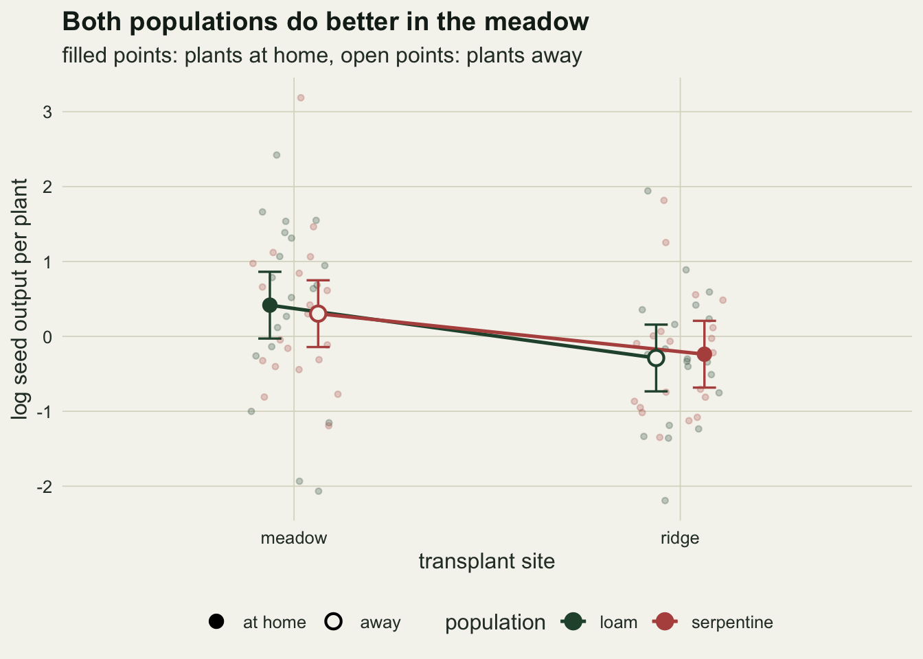
How often each reading finds adaptation that is not there
One dataset shows the mechanism. The rate needs many, and it needs the size of the nuisance effect to vary, because a site that halves seed output is only one possible difference. Both main effects are swept from zero to the size of a threefold difference in seed output, one at a time, with the local adaptation held at zero. Every rate below comes from 20000 simulated transplants per point, a count fixed before any rate was looked at.
n_rep <- 20000
eff_grid <- seq(0, log(3), length.out = 12)
set.seed(7225)
sweep_site <- t(vapply(eff_grid, function(e) rules(sim_fast(n_rep, e, 0, 0)), numeric(9)))
sweep_pop  <- t(vapply(eff_grid, function(e) rules(sim_fast(n_rep, 0, e, 0)), numeric(9)))
set.seed(7226)
at_site <- rules(sim_fast(n_rep, halve, 0, 0))
at_pop  <- rules(sim_fast(n_rep, 0, halve, 0))
at_both <- rules(sim_fast(n_rep, halve, halve, 0))
at_none <- rules(sim_fast(n_rep, 0, 0, 0))
mcse <- function(p) sqrt(p * (1 - p) / n_rep)
exact_single <- function(mean_diff) pt(crit, df_res, ncp = mean_diff / sqrt(2 / n_cell),
                                       lower.tail = FALSE)
chk_gap <- max(abs(c(at_site["hva_L"] - exact_single(halve),
                     at_pop["lvf_M"] - exact_single(halve),
                     at_none["hva_L"] - alpha_lev, at_none["sa"] - alpha_lev)))
one_any_null <- 1 - (1 - alpha_lev)^2
# exact rate for two one sided tests sharing the pooled variance estimate
union_exact <- integrate(function(v) (1 - (1 - pnorm(crit * sqrt(v / df_res),
                                                   lower.tail = FALSE))^2) * dchisq(v, df_res),
                         0, Inf)$value
z_pop_hva <- (at_pop["hva_one"] - union_exact) / mcse(union_exact)
sa_dev <- max(abs(c(sweep_site[, "sa"], sweep_pop[, "sa"]) - alpha_lev))
each_max <- max(sweep_site[, c("hva_each", "lvf_each")], sweep_pop[, c("hva_each", "lvf_each")])
The shortcut agrees with the exact noncentral t rates for single contrasts to within 0.0022, against a Monte Carlo standard error of 0.0035 at worst.
With no effects of any kind, a single home vs away contrast rejects in 4.9 per cent of transplants and the interaction test in 4.9 per cent. The at least one reading of home vs away already runs at 9.5 per cent, and the at least one reading of local vs foreign at 9.5 per cent, because each gets two chances. Both are simulated draws of one exact rate: two one sided five per cent tests that share the pooled variance estimate reject at least once in 9.73 per cent of transplants, a shade under the 9.75 per cent two independent tests would give. The Monte Carlo standard error is 0.15 percentage points for a rate near five per cent and 0.21 for a rate near ten.
Now let the ridge halve every plant’s seed output. The loam population passes the home vs away test in 70.2 per cent of transplants, and the serpentine population in 0.01 per cent. The at least one reading therefore flags adaptation in 70.2 per cent of transplants that contain none. The local vs foreign reading of the same data flags it in 9.8 per cent, which is the same exact quantity as with no effects at all (9.73 per cent), because the site effect cancels from both local vs foreign contrasts. The interaction test flags it in 5.0 per cent.
Swap the nuisance. Make the sites equal and the serpentine population the weaker one, setting half the seed of the loam plants wherever it grows, as a small inbred outcrop population might. Now it is local vs foreign that fails: the loam plants beat the incomers in the meadow in 70.3 per cent of transplants, and the at least one reading flags adaptation in 70.3 per cent, while home vs away stays at 10.2 per cent. A population effect cannot move that rate, because each home vs away contrast compares a population with itself; the exact value is still 9.73 per cent, and the simulated rate sits 2.3 Monte Carlo standard errors from it, a large draw rather than an effect. With both nuisances at once, both readings flag it, at 70.3 and 70.3 per cent, and the interaction test at 5.0 per cent. Across all 24 points of both sweeps the interaction test stays within 0.44 percentage points of five per cent.
The strict forms behave differently. Asking that every population win at home, or that the local population win in every habitat, fired in at most 0.31 per cent of transplants anywhere along the sweeps. That is the answer to a question that is easy to get backwards. A site effect with no local adaptation cannot make both populations do better at home, because in expectation it pushes one home contrast up by exactly as much as it pushes the other one down; a double home advantage from that process needs sampling noise on both contrasts in the right direction at once. This is not a statement that a double home advantage is impossible under local adaptation. It is exactly what local adaptation looks like when the adaptation is larger than the difference between the sites.
rule_lev <- c("home vs away, at least one", "home vs away, every population",
              "local vs foreign, at least one", "local vs foreign, every habitat",
              "sympatric vs allopatric")
long_rates <- function(tab, nuisance) {
  data.frame(effect = rep(eff_grid, 5), nuisance = nuisance,
             rule = factor(rep(rule_lev, each = length(eff_grid)), levels = rule_lev),
             rate = c(tab[, "hva_one"], tab[, "hva_each"], tab[, "lvf_one"],
                      tab[, "lvf_each"], tab[, "sa"]))
}
sweep_df <- rbind(long_rates(sweep_site, "a poorer site"),
                  long_rates(sweep_pop, "a weaker population"))
rule_cols  <- setNames(c(te_rust, te_rust, te_gold, te_gold, te_forest), rule_lev)
rule_lines <- setNames(c("solid", "dashed", "solid", "dashed", "solid"), rule_lev)
ggplot(sweep_df, aes(effect, rate, colour = rule, linetype = rule)) +
  geom_hline(yintercept = alpha_lev, colour = te_body, linetype = "dotted", linewidth = 0.5) +
  geom_vline(xintercept = halve, colour = te_line, linewidth = 0.8) +
  geom_line(linewidth = 0.9) +
  facet_wrap(~ nuisance) +
  scale_colour_manual(values = rule_cols, name = NULL) +
  scale_linetype_manual(values = rule_lines, name = NULL) +
  guides(colour = guide_legend(nrow = 3), linetype = guide_legend(nrow = 3)) +
  labs(x = "main effect on log seed output (no local adaptation)",
       y = "rate of declaring local adaptation",
       title = "Each criterion is blind to one main effect only",
       subtitle = "dotted line: five per cent; grey line: half the seed") +
  theme_datasheet() +
  theme(legend.position = "bottom", strip.text = element_text(colour = te_ink, face = "bold"))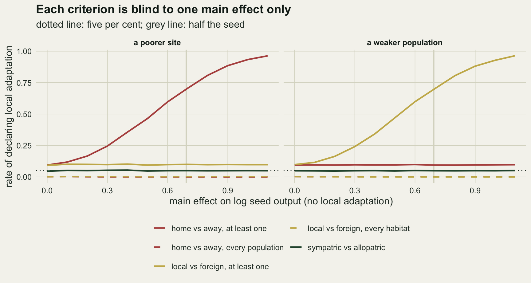
The strict criteria pay for their caution in power
A reading that never fires spuriously is only useful if it fires when it should. The second set of simulations adds genuine local adaptation, a sympatric advantage from zero up to a 2.5 fold difference in seed output between sympatric and allopatric combinations (the grey line in the figure marks a halving), in three settings: no main effects, the poorer ridge, and the weaker serpentine population.
sym_grid <- seq(0, log(2.5), length.out = 10)
set.seed(3318)
scen <- list("no main effects" = c(0, 0), "a poorer site" = c(halve, 0),
             "a weaker population" = c(0, halve))
power_df <- do.call(rbind, lapply(names(scen), function(nm) {
  tab <- t(vapply(sym_grid, function(d) rules(sim_fast(n_rep, scen[[nm]][1], scen[[nm]][2], d)),
                  numeric(9)))
  data.frame(sym = rep(sym_grid, 5),
             setting = factor(nm, levels = names(scen)),
             rule = factor(rep(rule_lev, each = length(sym_grid)), levels = rule_lev),
             rate = c(tab[, "hva_one"], tab[, "hva_each"], tab[, "lvf_one"],
                      tab[, "lvf_each"], tab[, "sa"]))
}))
set.seed(3319)
pw_none <- rules(sim_fast(n_rep, 0, 0, halve))
pw_site <- rules(sim_fast(n_rep, halve, 0, halve))
pw_pop  <- rules(sim_fast(n_rep, 0, halve, halve))
ratio_ncp <- sqrt(2)
seed_allo <- 1 / exp(halve)
The design value for this comparison is a sympatric advantage of 0.693 on the log scale, so that a plant away from home, or among foreigners, sets 0.50 times the seed it would set in a sympatric combination. With no main effects the interaction test detects it in 92.2 per cent of transplants. The strict home vs away criterion, both populations at home, detects it in 49.2 per cent, and the strict local vs foreign criterion in 49.6 per cent. The interaction contrast averages two differences, so its standard error is smaller than that of either single contrast by a factor of 1.414, and the strict criteria then need two separate successes on top.
Put the poorer ridge back. The interaction test stays at 92.4 per cent, and strict local vs foreign at 49.2 per cent, but strict home vs away collapses to 4.9 per cent. The site effect is as large as the adaptation, so the serpentine population’s expected home advantage is zero and it can only pass by luck. This is the boundary of the case Kawecki and Ebert describe, a population adapted to a poor habitat that does no better at home, or even better away, when the other habitat is richer; and it is why they count a pattern that meets local vs foreign but not home vs away as just as much support for local adaptation as one that meets both. The weaker population does the same thing to local vs foreign: strict local vs foreign falls to 4.8 per cent while strict home vs away holds at 49.7 per cent and the interaction test at 92.6 per cent.
The at least one readings look powerful on this figure, at 99.7 per cent for home vs away in the poorer site setting, but that line starts from its own false positive rate at zero adaptation, and a rule that fires in 70.2 per cent of transplants with no adaptation in them cannot be compared on power with a test at five per cent.
ggplot(power_df, aes(sym, rate, colour = rule, linetype = rule)) +
  geom_hline(yintercept = alpha_lev, colour = te_body, linetype = "dotted", linewidth = 0.5) +
  geom_vline(xintercept = halve, colour = te_line, linewidth = 0.8) +
  geom_line(linewidth = 0.9) +
  facet_wrap(~ setting) +
  scale_colour_manual(values = rule_cols, name = NULL) +
  scale_linetype_manual(values = rule_lines, name = NULL) +
  guides(colour = guide_legend(nrow = 3), linetype = guide_legend(nrow = 3)) +
  labs(x = "true sympatric advantage on log seed output",
       y = "rate of declaring local adaptation",
       title = "Only the interaction test ignores both main effects",
       subtitle = "dotted line: five per cent; grey line: the design value") +
  theme_datasheet() +
  theme(legend.position = "bottom", strip.text = element_text(colour = te_ink, face = "bold"))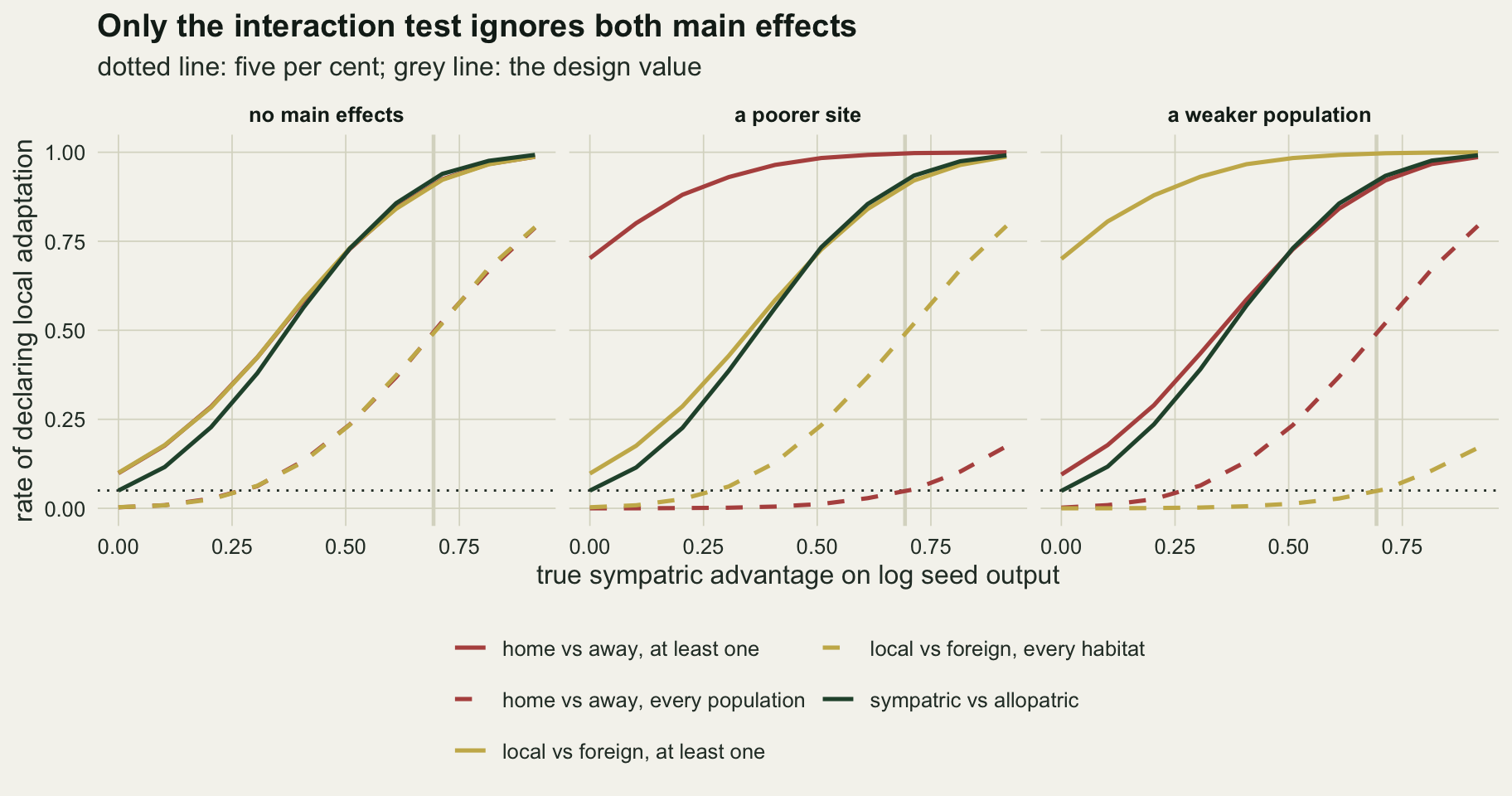
Plants are not the replicate for adaptation
Every test so far uses the plant as the unit: the interaction is judged against the scatter of plants within the four cells, with 76 degrees of freedom. That answers a narrower question than the write-up asks. It says whether these two populations respond differently to these two sites, and in the simulations above such a difference could only come from local adaptation, because the cell means contained nothing else. Real populations can differ in their response to two sites for reasons unrelated to the habitat they came from: drift at loci whose effects depend on the site, a genetic background that happens to suit one soil, seed provisioning that matters more on poor ground. With one population per habitat, a departure like that is the whole interaction, and the sympatric vs allopatric contrast cannot tell it from adaptation. This is the problem of pseudoreplication at the level of populations.
Blanquart and colleagues state the remedy: the sympatric vs allopatric effect is tested against the remainder of the population by site interaction, not against the error among individuals, because the population is the unit of replication. That needs several populations from each habitat. The simulation below gives every population and site combination a departure drawn independently with mean zero and standard deviation tau on the log seed scale, so there is still no local adaptation anywhere, and compares three analyses. The first is the two by two above with its plant level test. The second has four populations from each habitat, each planted at both sites, with the same total number of plants spread over them, still tested at plant level. The third is the same replicated design tested at population level: population, site and a sympatric indicator fitted to the cell means, so that the sympatric vs allopatric contrast is judged against what is left of the population by site interaction.
tau_grid <- seq(0, 0.4, length.out = 9)   # sd of a non adaptive population by site departure
tau_ref  <- 0.2
k_many   <- 4                             # populations from each habitat
n_many   <- n_cell / k_many               # plants per population and site: same total
# each population planted at meadow and ridge; d = meadow minus ridge per population
sim_many <- function(n_rep, k, n_plants, tau, sym_eff) {
  v_cell <- sigma_res^2 / n_plants + tau^2
  d_mo <- matrix(rnorm(n_rep * k,  sym_eff, sqrt(2 * v_cell)), n_rep)   # meadow origin
  d_ro <- matrix(rnorm(n_rep * k, -sym_eff, sqrt(2 * v_cell)), n_rep)   # ridge origin
  est <- (rowMeans(d_mo) - rowMeans(d_ro)) / 2                          # sympatric minus allopatric
  df_plant <- 4 * k * (n_plants - 1)
  s2_plant <- sigma_res^2 * rchisq(n_rep, df_plant) / df_plant
  t_plant  <- est / sqrt(s2_plant / (n_plants * k))
  out <- c(plant = mean(t_plant > qt(1 - alpha_lev, df_plant)), pop = NA_real_)
  if (k > 1) {
    s2_diff <- (rowSums((d_mo - rowMeans(d_mo))^2) + rowSums((d_ro - rowMeans(d_ro))^2)) /
               (2 * k - 2)
    t_pop <- est / sqrt(s2_diff / (2 * k))
    out["pop"] <- mean(t_pop > qt(1 - alpha_lev, 2 * k - 2))
  }
  out
}
set.seed(4417)
gxe_tab <- t(vapply(tau_grid, function(tau) {
  c(two_plant = sim_many(n_rep, 1, n_cell, tau, 0)[["plant"]],
    many      = sim_many(n_rep, k_many, n_many, tau, 0))
}, numeric(3)))
colnames(gxe_tab) <- c("two_plant", "many_plant", "many_pop")
ref_row <- which.min(abs(tau_grid - tau_ref))
pop_dev <- max(abs(gxe_tab[, "many_pop"] - alpha_lev))

set.seed(4418)
pw_many_0   <- sim_many(n_rep, k_many, n_many, 0, halve)
pw_many_ref <- sim_many(n_rep, k_many, n_many, tau_ref, halve)
pw_two_ref  <- sim_many(n_rep, 1, n_cell, tau_ref, halve)

# the population level test is lm() on the cell means with a sympatric indicator
set.seed(4419)
cells <- expand.grid(pop = factor(seq_len(2 * k_many)), site = c("meadow", "ridge"))
cells$origin <- ifelse(as.integer(cells$pop) <= k_many, "meadow", "ridge")
cells$sym <- as.numeric(cells$origin == cells$site)
cells$mean_seed <- rnorm(2 * k_many, 0, 0.5)[cells$pop] + 0.4 * (cells$site == "meadow") +
  halve * (cells$sym - 0.5) + rnorm(nrow(cells), 0, tau_ref) +
  rnorm(nrow(cells), 0, sigma_res / sqrt(n_many))
fit_pop <- lm(mean_seed ~ pop + site + sym, data = cells)
wide <- tapply(cells$mean_seed, list(cells$pop, cells$site), identity)
d_all <- wide[, "meadow"] - wide[, "ridge"]
d_mo <- d_all[1:k_many]; d_ro <- d_all[-(1:k_many)]
est_hand <- (mean(d_mo) - mean(d_ro)) / 2
s2_hand  <- (sum((d_mo - mean(d_mo))^2) + sum((d_ro - mean(d_ro))^2)) / (2 * k_many - 2)
pop_gap  <- abs(est_hand / sqrt(s2_hand / (2 * k_many)) -
                summary(fit_pop)$coefficients["sym", "t value"])
The replicated design has 5 plants per population and site, 80 plants in all as in the two by two, and 16 cell means. The shortcut for the population level test matches the t value of lm() fitted to the cell means to 4.4e-16, with 6 residual degrees of freedom. With no departures all three analyses hold their level, at 5.1, 5.0 and 5.2 per cent. With departures of standard deviation 0.2, the plant level test of the two by two declares local adaptation in 10.3 per cent of transplants that contain none, and at 0.4 in 21.4 per cent. Spreading the same plants over 8 populations dilutes the departures but does not remove them: the plant level test there reaches 6.7 and 10.9 per cent. The population level test stays within 0.24 percentage points of five per cent across the whole grid.
The price is paid in power. At the design value of local adaptation with no departures, the population level test detects it in 86.3 per cent of transplants, 5.9 percentage points below the 92.2 per cent of the plant level test of the two by two, because it has 6 degrees of freedom for its error and not 76; with departures of standard deviation 0.2 it detects it in 80.1 per cent. The plant level two by two still reports 85.6 per cent in that setting, but a detection rate from a test that also fires in 10.3 per cent of transplants with no adaptation is not power.
gxe_df <- data.frame(tau = rep(tau_grid, 3),
                     analysis = factor(rep(c("two populations, plant level",
                                             "eight populations, plant level",
                                             "eight populations, population level"),
                                           each = length(tau_grid)),
                                       levels = c("two populations, plant level",
                                                  "eight populations, plant level",
                                                  "eight populations, population level")),
                     rate = c(gxe_tab[, "two_plant"], gxe_tab[, "many_plant"], gxe_tab[, "many_pop"]))
ggplot(gxe_df, aes(tau, rate, colour = analysis)) +
  geom_hline(yintercept = alpha_lev, colour = te_body, linetype = "dotted", linewidth = 0.5) +
  geom_line(linewidth = 0.9) +
  geom_point(size = 2) +
  scale_colour_manual(values = c(te_rust, te_gold, te_forest), name = NULL) +
  guides(colour = guide_legend(nrow = 2)) +
  labs(x = "sd of the non adaptive population by site departure (log seed output)",
       y = "rate of declaring local adaptation",
       title = "Tested against plants, a non adaptive interaction looks adaptive",
       subtitle = "no local adaptation in any transplant; dotted line: five per cent") +
  theme_datasheet() + theme(legend.position = "bottom")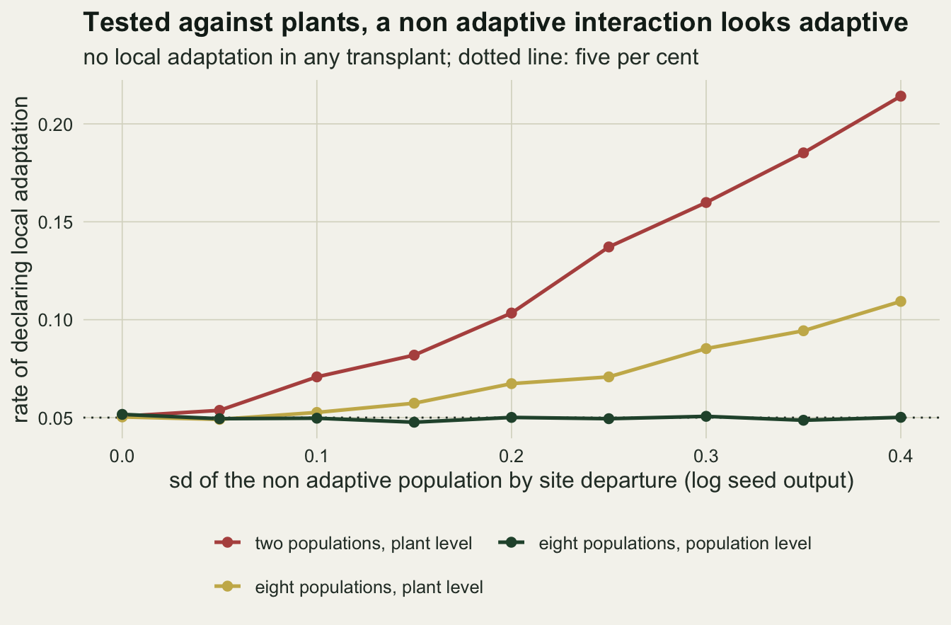
What to report
Report the four cell means with their intervals, not a verdict. A reader who has the four numbers can compute both criteria, both main effects and the interaction; a reader who has only “the loam population performed better at home” has a number with a site effect of unknown size inside it.
Test local adaptation with the sympatric vs allopatric contrast, with its estimate, standard error and one sided p value, in a model that also carries population and site effects; at the design value above it had more power than either strict criterion in every setting. What it is tested against decides what it can claim. In a two by two design the only error available is the scatter of plants, so the test (one coefficient of an lm() with sum to zero contrasts, or the interaction line of anova(), halved for direction) says whether these two populations differ in their response to these two sites. It kept its level whatever the main effects did only because the simulated cells held no other interaction; a non adaptive departure of standard deviation 0.2 already took it to 10.3 per cent. Report it as that difference, not as adaptation. A claim about adaptation to habitat needs several populations from each habitat, with the contrast tested against the rest of the population by site interaction, which in a balanced design is lm() on the cell means with population, site and a sympatric indicator.
Report both main effects alongside it, as descriptions of the sites and the populations. A large site effect is ecology worth reporting in its own right, and it tells the reader in advance that home vs away will be misleading in this system. A large population effect points to something other than divergent selection: inbreeding, maternal provisioning of the seed, or a collection that sampled a poor year.
If a criterion is quoted at all, quote it in the strict form and say which one. A home advantage in one population out of two is not evidence of local adaptation, and neither is a local advantage at one site out of two.
Honest limits
The criteria and their failure rates are measured only in a two by two design, which Blanquart and colleagues do not recommend for testing local adaptation: four fitness measures leave no degrees of freedom to test the sympatric vs allopatric contrast once habitat and population quality are accounted for. The two by two here is a device for seeing the algebra. They also point out that Kawecki and Ebert’s requirement that every population meet the local vs foreign pattern grows more stringent as more populations are sampled; the strict criteria were not simulated with more than two populations, so that is not measured here. The replicated design in the last section is one configuration (4 populations from each habitat, one site per habitat, equal plants per cell), chosen before running.
The response is log seed output with normal errors and equal variance in every cell. Real fitness data are counts with many zeros, survival is usually part of fitness, and a poorer site often inflates variance as well as reducing the mean. A generalised linear model changes the scale on which main effects and interaction are defined, and an interaction on the log scale is not an interaction on the count scale, so the choice of scale is part of the definition of local adaptation and not a technical detail.
The plants are independent. In a real transplant they sit in blocks and come from maternal families, and families nested in populations belong in the model as random effects, which changes the degrees of freedom of the population comparison. With one population per habitat type, population and habitat of origin are completely confounded, so the population effect cannot be separated from any other difference between the two collections. The replicated design treats the departures as independent across populations; populations from the same habitat that share ancestry, or sit close together, would carry correlated departures and take the population level test above its level too. It also still has one site per habitat, so a site that happens to favour the populations from one habitat for reasons unrelated to that habitat looks like adaptation; replicating sites within habitats is the matching fix, and it is not simulated here.
The one sided tests at five per cent are a choice; Blanquart and colleagues use two sided tests. Two sided tests at five per cent, read only in the direction of adaptation, halve the single contrast rates at zero effect and lower the power curves, but they do not change the structure: each criterion still carries one main effect in full.
References
Kawecki TJ, Ebert D 2004 Ecology Letters 7(12):1225-1241 (10.1111/j.1461-0248.2004.00684.x)
Blanquart F, Kaltz O, Nuismer SL, Gandon S 2013 Ecology Letters 16(9):1195-1205 (10.1111/ele.12150)
Hereford J 2009 The American Naturalist 173(5):579-588 (10.1086/597611)