library(ggplot2)

te_pal <- list(forest = "#275139", green = "#2f8f63", sage = "#93a87f",
               clay = "#b5534e", gold = "#cda23f", line = "#dad9ca",
               ink = "#16241d", paper = "#f5f4ee")

theme_te <- function() {
  theme_minimal(base_size = 12) +
    theme(panel.grid.minor = element_blank(),
          panel.grid.major = element_line(colour = "#e7e6dc"),
          plot.background = element_rect(fill = "#f5f4ee", colour = NA),
          panel.background = element_rect(fill = "#f5f4ee", colour = NA),
          plot.title = element_text(face = "bold", colour = te_pal$ink),
          axis.title = element_text(colour = "#2c3a31"),
          axis.text = element_text(colour = "#2c3a31"))
}Term order in unbalanced factorial ANOVA
R
ANOVA
linear models
experimental design
ecology tutorial
Unequal cell counts make anova() return different p-values for the same fitted model when the terms are reordered. A simulation measures how often it matters.
A grassland experiment was laid out in the spring of 2023 as a full factorial: grazing exclusion crossed with nutrient addition, twelve plots in each of the four combinations, forty-eight two-metre squares on one hillside. Fenced plots got a wire exclosure, open plots got nothing, half of each group got an annual NPK dose and half got none. Aboveground biomass was clipped, dried and weighed at peak standing crop in the third season. The design as written on the plan is balanced, and a balanced two-factor design is the easiest thing in applied statistics to analyse.
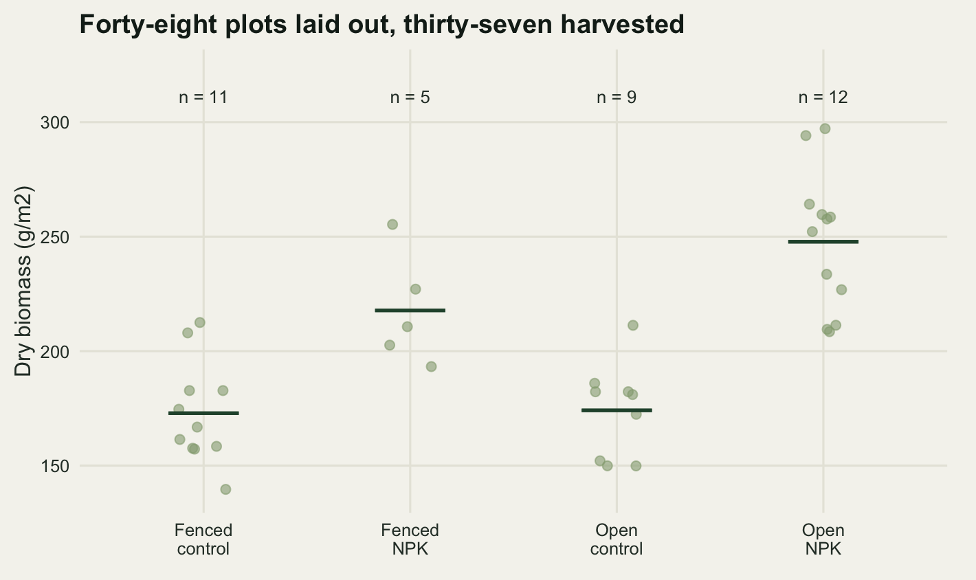
The design as harvested is not the design as written. Roe deer pushed through the netting on seven of the twelve fenced plots that were also fertilised, which is not bad luck so much as the obvious consequence of putting the best forage on the hill behind a fence a deer can lean on. Those plots were struck out because the treatment did not hold. A summer storm put the lower corner of the site under water for four days and three open unfertilised plots were abandoned. One fenced unfertilised plot had its exclosure cut and removed. Thirty-seven plots reached the drying oven, spread across the four cells as eleven, five, nine and twelve.
Nothing about that is exotic. Plots go missing from field experiments for reasons that have nothing to do with the analyst, and they rarely go missing evenly. What follows from it is less obvious: with unequal cell counts, anova(lm(biomass ~ grazing * nutrients)) and anova(lm(biomass ~ nutrients * grazing)) return different p-values for the main effects, from the same data, on a model that is identical in every other respect. The residuals match to the last digit, the fitted values match, the overall F matches, and the table does not.
This post measures three things: how large the gap between the two orders gets, how often it carries the 0.05 verdict with it, and what happens when the usual escape route, a Type III table, is taken without changing the contrast coding first.
Three neighbouring posts set the boundaries. Contrasts and post-hoc comparisons already teaches contr.sum as a coding choice and what it does to the coefficients, so contrast coding is a prerequisite here rather than a topic; this post is about which hypothesis a table is testing, and the coding turns out to decide that. t-tests and ANOVA as linear models builds the analysis of variance table that is about to be shown to be order-dependent, on balanced data where the problem cannot arise. Split-plot designs starts from the same trigger, balance being the first thing a field season destroys, but the mechanism there is error strata and the mechanism here is non-orthogonality within one design matrix.
The design that came out of the field
Everything below runs on synthetic biomass, because the point of the exercise is to compare what a table says against a truth that was set rather than inferred. The generating values are ordinary for a lowland grassland: unfertilised standing crop near 180 g/m2, an NPK response of 55 g/m2, and plot-to-plot variation of 28 g/m2 around the cell mean. The grazing effect is set to exactly zero for now, so every significant grazing result in this section is a false positive by construction.
lv_grazing <- c("fenced", "open")
lv_nutrient <- c("control", "npk")
cells <- expand.grid(nutrients = factor(lv_nutrient, levels = lv_nutrient),
                     grazing = factor(lv_grazing, levels = lv_grazing))

nn_real <- c(11, 5, 9, 12)
design <- cells[rep(seq_len(4), nn_real), ]
rownames(design) <- NULL
gz <- as.numeric(design$grazing == "open")
nu <- as.numeric(design$nutrients == "npk")
npl <- nrow(design)

plots_intended <- 48
npk_eff <- 55
sd_plot <- 28
base_crop <- 180
d_head <- 35

cell_n <- table(design$grazing, design$nutrients)
print(cell_n)
         control npk
  fenced      11   5
open 9 12print(c(intended = plots_intended, harvested = npl, lost = plots_intended - npl)) intended harvested lost
48 37 11 37 plots of the 48 that were marked out reached the balance, so 11 were lost. The cell counts are 11, 5, 9 and 12.
The quantity that decides whether term order matters is not how uneven those counts are. It is whether they are proportional. Two factors are orthogonal in the design matrix when the cell counts satisfy \(n_{11}n_{22} = n_{12}n_{21}\), that is, when the table of counts is what you would get by multiplying a row profile by a column profile. A proportionally unbalanced design is still orthogonal, and the sequential table is still order-free.
cross_gap <- function(nvec) nvec[1] * nvec[4] - nvec[2] * nvec[3]
col_cor <- function(nvec) {
  dg <- cells[rep(seq_len(4), nvec), ]
  X <- model.matrix(~ grazing + nutrients, data = dg)
  unname(cor(X[, 2], X[, 3]))
}

nn_prop <- c(12, 6, 10, 5)
print(rbind(realised = nn_real, proportional = nn_prop))
[,1] [,2] [,3] [,4]
realised 11 5 9 12
proportional 12 6 10 5print(round(c(cross_gap_realised = cross_gap(nn_real),
cross_gap_proportional = cross_gap(nn_prop),
column_cor_realised = col_cor(nn_real),
column_cor_proportional = col_cor(nn_prop)), 6)) cross_gap_realised cross_gap_proportional column_cor_realised
87.000000 0.000000 0.257401
column_cor_proportional
0.000000 The proportional layout 12, 6, 10, 5 is more lopsided than the realised one in raw counts, 33 plots against 37, and it loses more than half of one cell. It is nonetheless orthogonal: 0 for the cross-product gap, and a correlation of 0 between the coded grazing and nutrient columns. The realised design has a gap of 87 and a column correlation of 0.2574. That correlation is the whole mechanism: once the two predictors share information, the amount of variation credited to each depends on which one is allowed to claim the shared part.
worked <- design
set.seed(20260804)
worked$biomass <- base_crop + 0 * gz + npk_eff * nu + rnorm(npl, 0, sd_plot)

cell_mean <- tapply(worked$biomass, list(worked$grazing, worked$nutrients), mean)
print(round(cell_mean, 2))
control npk
fenced 172.88 217.79
open 174.12 247.78marg_fenced <- mean(worked$biomass[worked$grazing == "fenced"])
marg_open <- mean(worked$biomass[worked$grazing == "open"])
print(round(c(marginal_fenced = marg_fenced, marginal_open = marg_open,
marginal_gap = marg_open - marg_fenced), 3))marginal_fenced marginal_open marginal_gap
186.913 216.209 29.296 Within each grazing level the fertiliser response is plain, 44.9 g/m2 behind the fence and 73.7 g/m2 outside it. Within each nutrient level the grazing comparison is noise around the zero that was put in, 1.2 g/m2 on unfertilised ground and 30 g/m2 on fertilised ground, the second of those resting on the 5 fenced plots that survived.
The marginal comparison is a different matter. Averaging over nutrients without regard to the cell counts gives fenced plots 186.9 g/m2 and open plots 216.2 g/m2, a gap of 29.3 g/m2 where the truth is zero. The open group simply contains a higher proportion of fertilised plots, 12 out of 21 against 5 out of 16, and the fertiliser response has leaked into the grazing contrast.
The same fit, two tables
anova() applied to a single lm object gives sequential sums of squares, called Type I in the naming scheme that goes back to the SAS documentation of the 1970s. Each term is credited with the reduction in residual sum of squares it produces when it is added to everything above it in the table and nothing below it. That description contains the problem in plain sight: what a term is credited with depends on what came before it, and what came before it is whatever the person typing the formula happened to write first.
fit_gn <- lm(biomass ~ grazing * nutrients, data = worked)
fit_ng <- lm(biomass ~ nutrients * grazing, data = worked)

a_gn <- anova(fit_gn)
a_ng <- anova(fit_ng)
print(a_gn)
Analysis of Variance Table
Response: biomass
Df Sum Sq Mean Sq F value Pr(>F)
grazing 1 7794 7794 12.2975 0.001331 **
nutrients 1 33131 33131 52.2771 2.722e-08 ***
grazing:nutrients 1 1703 1703 2.6872 0.110659
Residuals 33 20914 634
---
Signif. codes: 0 '***' 0.001 '**' 0.01 '*' 0.05 '.' 0.1 ' ' 1print(a_ng)Analysis of Variance Table
Response: biomass
Df Sum Sq Mean Sq F value Pr(>F)
nutrients 1 39446 39446 62.2413 4.268e-09 ***
grazing 1 1479 1479 2.3334 0.1362
nutrients:grazing 1 1703 1703 2.6872 0.1107
Residuals 33 20914 634
---
Signif. codes: 0 '***' 0.001 '**' 0.01 '*' 0.05 '.' 0.1 ' ' 1The grazing main effect is significant at 0.00133 when grazing is written first and not significant at 0.1362 when it is written second. The sums of squares that produce those, 7793.6 and 1478.8, differ by a factor of 5.27. The nutrient effect moves too, from 39446 when it goes first to 33131 when it goes second, though it is so large that no verdict changes.
Before drawing any conclusion from that, it is worth establishing that the two are the same model and not two different analyses.
same_resid <- isTRUE(all.equal(residuals(fit_gn), residuals(fit_ng)))
same_fitted <- isTRUE(all.equal(fitted(fit_gn), fitted(fit_ng)))
same_sigma <- isTRUE(all.equal(summary(fit_gn)$sigma, summary(fit_ng)$sigma))
same_r2 <- isTRUE(all.equal(summary(fit_gn)$r.squared, summary(fit_ng)$r.squared))
same_overall <- isTRUE(all.equal(unname(summary(fit_gn)$fstatistic),
                                 unname(summary(fit_ng)$fstatistic)))
max_fitted_gap <- max(abs(fitted(fit_gn) - fitted(fit_ng)))

print(c(residuals = same_resid, fitted = same_fitted, resid_sd = same_sigma,
        r_squared = same_r2, overall_F = same_overall))
residuals fitted resid_sd r_squared overall_F
TRUE TRUE TRUE TRUE TRUE print(round(c(overall_F = unname(summary(fit_gn)$fstatistic[1]),
r_squared = summary(fit_gn)$r.squared,
resid_sd = summary(fit_gn)$sigma,
interaction_SS_order1 = a_gn["grazing:nutrients", "Sum Sq"],
interaction_SS_order2 = a_ng["nutrients:grazing", "Sum Sq"]), 5)) overall_F r_squared resid_sd
22.42061 0.67086 25.17450
interaction_SS_order1 interaction_SS_order2
1703.01696 1703.01696 print(formatC(max_fitted_gap, format = "e", digits = 2))[1] "5.68e-14"Residuals identical, fitted values identical to within 5.68e-14, residual standard deviation 25.174 in both, overall F of 22.421 on the same degrees of freedom in both, and an interaction sum of squares of 1703 in both, because the last term in a sequential table is adjusted for everything and so has nowhere left to move. There is one fit. The difference is entirely in how its explained variation is divided between two correlated columns, and the division is settled by typing order.
The two grazing sums of squares have names. The larger one, grazing listed first, is the effect of grazing ignoring nutrients: it is the marginal comparison computed above, fertiliser leakage included. The smaller one, grazing listed last among the main effects, is the effect of grazing adjusted for nutrients, which is what almost everyone means when they say main effect. That second quantity has a second name as well, and it is worth recording now because it saves a package later.
rss <- function(fo) sum(residuals(lm(fo, data = worked))^2)
ss2_grazing <- rss(biomass ~ nutrients) - rss(biomass ~ grazing + nutrients)
ss2_nutrient <- rss(biomass ~ grazing) - rss(biomass ~ grazing + nutrients)

print(round(c(hand_built_grazing = ss2_grazing,
              anova_second_listed = a_ng["grazing", "Sum Sq"],
              hand_built_nutrient = ss2_nutrient,
              anova_second_listed_nutrient = a_gn["nutrients", "Sum Sq"]), 6))
hand_built_grazing anova_second_listed
1478.79 1478.79
hand_built_nutrient anova_second_listed_nutrient
33130.88 33130.88 In a two-factor model, the Type II sum of squares for a factor is exactly its sequential sum of squares when it is listed last among the main effects. Type II adjusts each main effect for the other main effect and for nothing else, ignoring the interaction; the sequential table with the factor written second does precisely that. So anova(lm(y ~ B * A)) already contains the Type II test for A, and no extra machinery is needed to get it.
How often the order decides the verdict
One dataset settles nothing, so the experiment gets run four thousand times. The design is held fixed at the counts that came out of the field, since the imbalance is a property of the harvest rather than a random variable to be redrawn; only the biomass is resampled. The grazing effect stays at zero throughout, so both tests are testing a true null.
n_rep <- 4000
p_first <- numeric(n_rep)
p_last <- numeric(n_rep)
sim_dat <- design

set.seed(4021)
for (rep_i in seq_len(n_rep)) {
  sim_dat$biomass <- base_crop + npk_eff * nu + rnorm(npl, 0, sd_plot)
  p_first[rep_i] <- anova(lm(biomass ~ grazing * nutrients,
                             data = sim_dat))["grazing", "Pr(>F)"]
  p_last[rep_i] <- anova(lm(biomass ~ nutrients * grazing,
                            data = sim_dat))["grazing", "Pr(>F)"]
}

med_ratio <- median(pmax(p_first, p_last) / pmin(p_first, p_last))
med_signed <- median(p_last / p_first)
q90_ratio <- unname(quantile(p_last / p_first, 0.9))
flip_rate <- mean((p_first < 0.05) != (p_last < 0.05))
flip_up <- mean(p_first < 0.05 & p_last >= 0.05)
flip_down <- mean(p_first >= 0.05 & p_last < 0.05)
rej_first <- mean(p_first < 0.05)
rej_last <- mean(p_last < 0.05)
mc_se <- sqrt(flip_rate * (1 - flip_rate) / n_rep)

print(round(c(median_ratio = med_ratio, median_signed_ratio = med_signed,
              upper_decile_ratio = q90_ratio), 4))
median_ratio median_signed_ratio upper_decile_ratio
7.6683 6.3324 36.8340 print(round(c(flip_rate = flip_rate, flip_to_significant = flip_up,
flip_to_null = flip_down, monte_carlo_se = mc_se), 5)) flip_rate flip_to_significant flip_to_null monte_carlo_se
0.33075 0.30875 0.02200 0.00744 print(round(c(rejection_grazing_first = rej_first,
rejection_grazing_last = rej_last), 5))rejection_grazing_first rejection_grazing_last
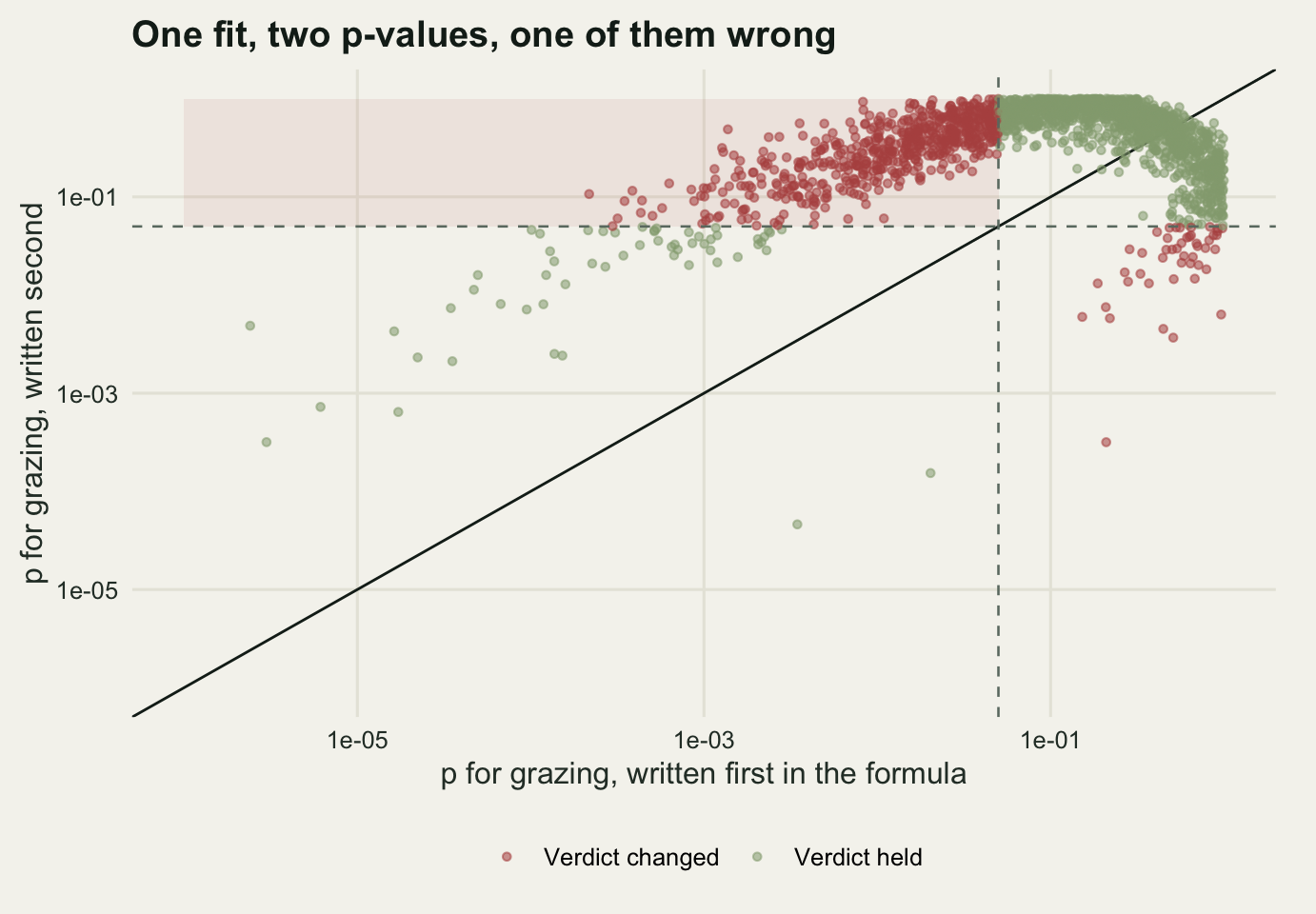
0.33425 0.04750 Over 4000 replicates the two p-values for the same effect on the same data differ by a median factor of 7.67, and in the upper decile the adjusted p-value is 36.8 times the unadjusted one. The 0.05 verdict changes in 33.1 per cent of replicates, with a Monte Carlo standard error of 0.74 percentage points, so that figure is pinned to within about one and a half percentage points either way. Almost all of the flipping runs one way: 30.9 per cent of replicates are significant with grazing first and not significant with grazing last, against 2.2 per cent the other way.
The rejection rates say which of the two is the one to worry about. Listing grazing last rejects a true null 4.8 per cent of the time, which is the nominal five per cent. Listing it first rejects 33.4 per cent of the time. That is not a subtlety about which sum of squares is more elegant. It is a false positive rate 7 times the advertised one, produced by nothing more than the order in which two factor names were typed into a formula, on a design that lost eleven plots to deer and weather.
How much imbalance it takes
The realised design lost seven of twelve fertilised exclosures. A reasonable question is whether that is an unusually bad case or an ordinary one, so the sweep is repeated with the other three cells held at their realised counts and the fertilised exclosure cell walked from twelve surviving plots down to three.
surv_grid <- 12:3
n_rep_g <- 1200
grad <- data.frame(surviving = surv_grid, column_cor = NA_real_,
                   median_ratio = NA_real_, flip = NA_real_, rejection = NA_real_)

for (j in seq_along(surv_grid)) {
  nn_j <- c(nn_real[1], surv_grid[j], nn_real[3], nn_real[4])
  dg <- cells[rep(seq_len(4), nn_j), ]
  nu_j <- as.numeric(dg$nutrients == "npk")
  m_j <- nrow(dg)
  pa <- numeric(n_rep_g)
  pb <- numeric(n_rep_g)
  set.seed(7100 + j)
  for (rep_i in seq_len(n_rep_g)) {
    dg$biomass <- base_crop + npk_eff * nu_j + rnorm(m_j, 0, sd_plot)
    pa[rep_i] <- anova(lm(biomass ~ grazing * nutrients,
                          data = dg))["grazing", "Pr(>F)"]
    pb[rep_i] <- anova(lm(biomass ~ nutrients * grazing,
                          data = dg))["grazing", "Pr(>F)"]
  }
  grad$column_cor[j] <- col_cor(nn_j)
  grad$median_ratio[j] <- median(pmax(pa, pb) / pmin(pa, pb))
  grad$flip[j] <- mean((pa < 0.05) != (pb < 0.05))
  grad$rejection[j] <- mean(pa < 0.05)
}

print(round(grad, 4))
surviving column_cor median_ratio flip rejection
1 12 0.0498 1.4917 0.0408 0.0700
2 11 0.0716 1.8059 0.0567 0.0758
3 10 0.0953 2.1480 0.0833 0.0925
4 9 0.1214 2.6354 0.1033 0.1292
5 8 0.1502 3.2524 0.1508 0.1525
6 7 0.1821 4.2829 0.1958 0.1925
7 6 0.2176 5.3722 0.2608 0.2533
8 5 0.2574 7.1587 0.3267 0.3275
9 4 0.3024 10.2023 0.4000 0.4033
10 3 0.3536 16.8916 0.5283 0.5125row_full <- which(grad$surviving == 12)
row_real <- which(grad$surviving == nn_real[2])
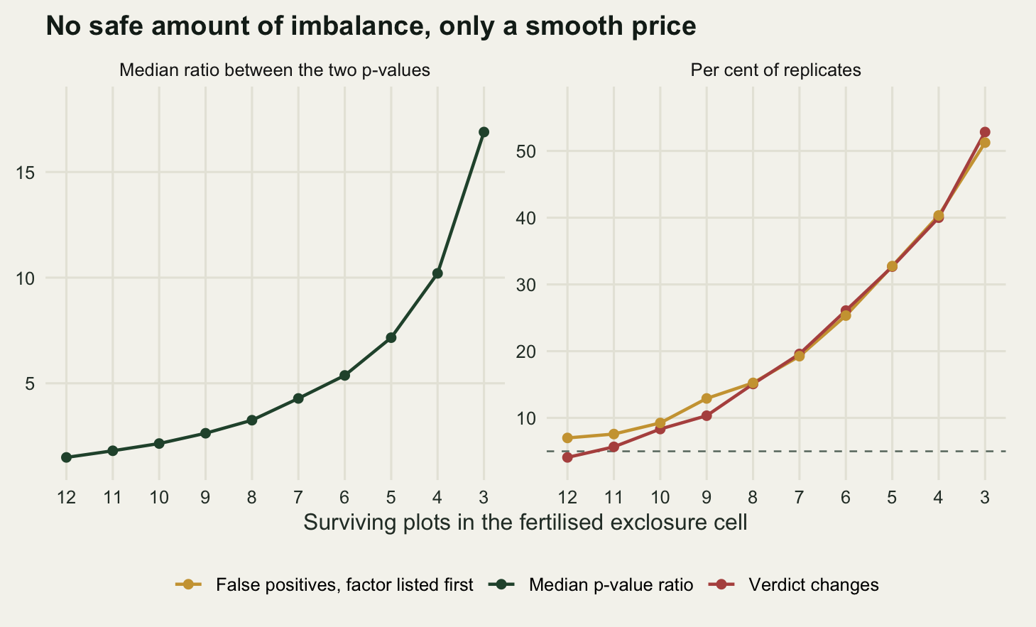
row_worst <- which(grad$surviving == 3)With all twelve fertilised exclosures intact the design is still unbalanced, 11, 12, 9 and 12, and the column correlation is 0.0498. That residual imbalance already costs something: a median p-ratio of 1.49, a flip rate of 4.1 per cent and a false positive rate of 7 per cent for the first-listed factor. The four plots lost to a cut fence and a flooded corner, out of 48, are enough on their own to run the nominal five per cent test at 1.4 times its advertised size.
At the realised 5 surviving plots the correlation is 0.257, the median ratio is 7.16 and the flip rate 32.7 per cent. Down at three the correlation reaches 0.354, the median ratio 16.9, and the verdict changes in 52.8 per cent of replicates: the first-listed factor is then rejecting a true null more often than not, at 51.2 per cent.
The curve has no threshold in it, no level of imbalance below which the sequential table is safe and above which it is not, which is why the habit of glancing at the cell counts and deciding they look close enough does not work. The only safe value is proportionality, and that is a knife edge a real harvest never lands on.
Building the other tables without a package
The usual advice at this point is to fit the model and call Anova() from the car package, which produces Type II and Type III tables directly. That is what most ecologists do, and it is a sensible default. It is not used here, partly because the point of this blog is to write the estimator out rather than call it, and partly because a Type III table produced by a function whose internals you have not read is exactly how the trap in the next section gets sprung. Anyone with car installed can put these numbers side by side with Anova(fit_gn, type = 2) and Anova(fit_gn, type = 3) on their own machine; they agree.
The general recipe for a marginal test is a comparison of two design matrices rather than two formulas, and the distinction matters. Take the model matrix of the full fit, find the columns that belong to the term of interest through the assign attribute, drop exactly those columns, refit, and compare residual sums of squares against the full model’s residual mean square.
drop_term_test <- function(fit, term) {
  X <- model.matrix(fit)
  yv <- model.response(model.frame(fit))
  which_term <- which(attr(terms(fit), "term.labels") == term)
  keep <- attr(X, "assign") != which_term
  rss_full <- sum(residuals(fit)^2)
  df_full <- fit$df.residual
  rss_red <- sum(lm.fit(X[, keep, drop = FALSE], yv)$residuals^2)
  df_gap <- sum(!keep)
  f_val <- ((rss_red - rss_full) / df_gap) / (rss_full / df_full)
  c(SS = rss_red - rss_full, df = df_gap, F = f_val,
    p = pf(f_val, df_gap, df_full, lower.tail = FALSE))
}
Doing this by formula instead of by column fails silently on a two by two design. Removing the grazing main effect from biomass ~ grazing * nutrients and writing biomass ~ nutrients + grazing:nutrients does not produce a smaller model: the interaction term expands to two columns instead of one and the reduced formula has the same rank as the full one. The column-dropping version does what the formula version appears to promise.
options(contrasts = c("contr.treatment", "contr.poly"))
fit_treat <- lm(biomass ~ grazing * nutrients, data = worked)
t3_treat_grazing <- drop_term_test(fit_treat, "grazing")
t3_treat_nutrient <- drop_term_test(fit_treat, "nutrients")

coef_treat <- summary(fit_treat)$coefficients
print(round(coef_treat, 5))
Estimate Std. Error t value Pr(>|t|)
(Intercept) 172.87959 7.59040 22.77610 0.00000
grazingopen 1.23925 11.31509 0.10952 0.91345
nutrientsnpk 44.90686 13.57811 3.30730 0.00228
grazingopen:nutrientsnpk 28.75005 17.53840 1.63926 0.11066print(round(t3_treat_grazing, 6)) SS df F p
7.601934 1.000000 0.011995 0.913452 print(round(c(coefficient_p_grazingopen = coef_treat["grazingopen", "Pr(>|t|)"],
type3_p_grazing = unname(t3_treat_grazing["p"]),
coefficient_t_squared = coef_treat["grazingopen", "t value"]^2,
type3_F = unname(t3_treat_grazing["F"])), 6))coefficient_p_grazingopen type3_p_grazing coefficient_t_squared
0.913452 0.913452 0.011995
type3_F
0.011995 The Type III p-value for the grazing main effect under treatment contrasts is 0.9135. The p-value for the grazingopen coefficient is 0.9135. They are the same number, and the F is the square of the t. That identity is the whole problem, stated as compactly as it can be. Under contr.treatment, the grazingopen column of the design matrix is the indicator for open plots, and in the presence of the interaction its coefficient is the difference between open and fenced plots at the reference level of nutrients, that is, on unfertilised ground only. A Type III table computed under treatment contrasts labels that row grazing and calls it a main effect. It is a simple effect at one level of the other factor, and the five fertilised exclosure plots contribute nothing to it.
The trap, measured
The worked dataset had no interaction in it, so testing grazing at one nutrient level and testing it on average happen to ask nearly the same question. Now the truth is changed to a crossover: grazing raises standing crop by 35 g/m2 on unfertilised ground, where cropping keeps a light-limited sward open, and lowers it by the same amount on fertilised ground, where the removed biomass is no longer replaced. The unweighted average of those two simple effects is exactly zero, so a main effect of grazing, in the sense of an average over nutrient levels, does not exist.
d_grid <- c(0, 10, 20, 30, d_head, 40)
n_rep_t <- 1500
rej_treat <- numeric(length(d_grid))
rej_sum <- numeric(length(d_grid))

for (j in seq_along(d_grid)) {
  d_j <- d_grid[j]
  pt <- numeric(n_rep_t)
  ps <- numeric(n_rep_t)
  set.seed(9300 + j)
  for (rep_i in seq_len(n_rep_t)) {
    sim_dat$biomass <- base_crop + d_j * gz + npk_eff * nu -
      2 * d_j * gz * nu + rnorm(npl, 0, sd_plot)
    options(contrasts = c("contr.treatment", "contr.poly"))
    pt[rep_i] <- drop_term_test(lm(biomass ~ grazing * nutrients,
                                   data = sim_dat), "grazing")["p"]
    options(contrasts = c("contr.sum", "contr.poly"))
    ps[rep_i] <- drop_term_test(lm(biomass ~ grazing * nutrients,
                                   data = sim_dat), "grazing")["p"]
  }
  rej_treat[j] <- mean(pt < 0.05)
  rej_sum[j] <- mean(ps < 0.05)
}
options(contrasts = c("contr.treatment", "contr.poly"))

trap <- data.frame(crossover = d_grid, treatment = rej_treat, sum_coding = rej_sum)
print(round(trap, 4))
crossover treatment sum_coding
1 0 0.0460 0.0480
2 10 0.1307 0.0580
3 20 0.3420 0.0493
4 30 0.6527 0.0560
5 35 0.7527 0.0500
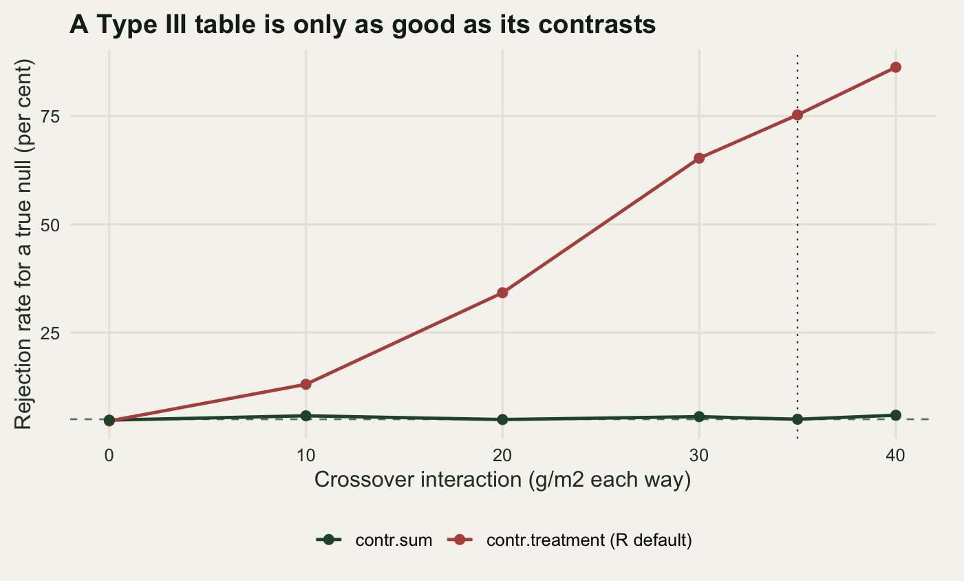
6 40 0.8627 0.0593row_head <- which(d_grid == d_head)At a crossover of 35 g/m2 the Type III test of the grazing main effect rejects a hypothesis that is true, by construction, in 75.3 per cent of 1500 replicates under R’s default contr.treatment. The same test under contr.sum rejects in 5 per cent, which is the nominal five. At a crossover of zero the two agree, 4.6 per cent against 4.8 per cent, since there is then no interaction for the coding to interact with. The gap opens as the interaction grows and it is monotone: the treatment-coded test is not noisy, it is answering a different question with increasing confidence.
The fix is one line, and it has to be run before the model is fitted, not after.
options(contrasts = c("contr.sum", "contr.poly"))
fit_sum <- lm(biomass ~ grazing * nutrients, data = worked)
fit_sum_rev <- lm(biomass ~ nutrients * grazing, data = worked)
t3_sum_grazing <- drop_term_test(fit_sum, "grazing")
t3_sum_rev <- drop_term_test(fit_sum_rev, "grazing")

options(contrasts = c("contr.treatment", "contr.poly"))
fit_tr_rev <- lm(biomass ~ nutrients * grazing, data = worked)
t3_treat_rev <- drop_term_test(fit_tr_rev, "grazing")

print(round(rbind(sum_forward = t3_sum_grazing, sum_reversed = t3_sum_rev,
                  treat_forward = t3_treat_grazing,
                  treat_reversed = t3_treat_rev), 6))
SS df F p
sum_forward 2009.303259 1 3.170472 0.084190
sum_reversed 2009.303259 1 3.170472 0.084190
treat_forward 7.601934 1 0.011995 0.913452
treat_reversed 7.601934 1 0.011995 0.913452print(formatC(c(sum_gap = unname(abs(t3_sum_grazing["p"] - t3_sum_rev["p"])),
treat_gap = unname(abs(t3_treat_grazing["p"] - t3_treat_rev["p"]))),
format = "e", digits = 2)) sum_gap treat_gap
"1.17e-15" "6.20e-14" Here is a result that the framing of this section does not lead you to expect, and it is worth stating flatly. The Type III p-value for grazing under sum coding is 0.0842 with grazing written first and 0.0842 with it written second; under treatment coding it is 0.9135 either way. The two differences are 1.17e-15 and 6.20e-14: zero to the last bit of a double, not merely small. Type III is order-invariant under either contrast scheme. It has to be, because the set of columns belonging to a term does not depend on where the term is written, so the model comparison is the same comparison either way, and order-invariance is the property Type III was invented to have.
That has a direct consequence for the self-test the practitioner is usually offered. Reordering the formula and checking that the answer holds is a genuine check on a sequential table, and it catches the failure measured two sections ago. It has no power at all against the contrast trap. A Type III table computed under treatment contrasts will pass the reordering check while reporting a test of grazing on unfertilised plots under the heading grazing. Two different defects, and only one of them is visible from the outside.
Which hypothesis each table answers
Everything so far can be put on one axis. Each test targets a specific linear combination of the four cell means, and the disagreements between them are disagreements about which combination deserves the name main effect of grazing. Setting the noise to zero makes the comparison exact.
noiseless <- design
noiseless$biomass <- base_crop + d_head * gz + npk_eff * nu - 2 * d_head * gz * nu
cell_true <- tapply(noiseless$biomass,
                    list(noiseless$grazing, noiseless$nutrients), mean)
print(cell_true)
control npk
fenced 180 235
open 215 200simple_control <- unname(cell_true["open", "control"] - cell_true["fenced", "control"])
simple_npk <- unname(cell_true["open", "npk"] - cell_true["fenced", "npk"])
target_first <- mean(noiseless$biomass[noiseless$grazing == "open"]) -
mean(noiseless$biomass[noiseless$grazing == "fenced"])
target_two <- unname(coef(lm(biomass ~ grazing + nutrients,
data = noiseless))["grazingopen"])
target_t3t <- unname(coef(lm(biomass ~ grazing * nutrients,
data = noiseless))["grazingopen"])
options(contrasts = c("contr.sum", "contr.poly"))
target_t3s <- unname(-2 * coef(lm(biomass ~ grazing * nutrients,
data = noiseless))["grazing1"])
options(contrasts = c("contr.treatment", "contr.poly"))
print(round(c(simple_effect_control = simple_control,
simple_effect_npk = simple_npk,
unweighted_average = (simple_control + simple_npk) / 2,
type1_first = target_first, type2 = target_two,
type3_treatment = target_t3t, type3_sum = target_t3s), 4))simple_effect_control simple_effect_npk unweighted_average
35.0000 -35.0000 0.0000
type1_first type2 type3_treatment
9.2411 5.8637 35.0000
type3_sum
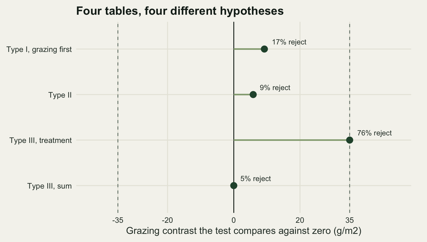
0.0000 The two simple effects are 35 and -35 g/m2, and their unweighted average is 0. The Type III test under treatment contrasts targets 35, the simple effect on unfertilised ground. Under sum contrasts it targets 0, the unweighted average. Type II targets 5.86, a weighted average whose weights come from the cell counts rather than from anything anyone chose, which lands near zero here but not on it. The first-listed sequential test targets 9.24, a quantity that mixes the grazing contrast with the nutrient response and has no interpretation at all.
n_rep_f <- 2000
p_four <- matrix(NA_real_, n_rep_f, 4)
colnames(p_four) <- c("Type I, grazing first", "Type II",
                      "Type III, treatment", "Type III, sum")

set.seed(6611)
for (rep_i in seq_len(n_rep_f)) {
  sim_dat$biomass <- base_crop + d_head * gz + npk_eff * nu -
    2 * d_head * gz * nu + rnorm(npl, 0, sd_plot)
  p_four[rep_i, 1] <- anova(lm(biomass ~ grazing * nutrients,
                               data = sim_dat))["grazing", "Pr(>F)"]
  p_four[rep_i, 2] <- anova(lm(biomass ~ nutrients * grazing,
                               data = sim_dat))["grazing", "Pr(>F)"]
  p_four[rep_i, 3] <- drop_term_test(lm(biomass ~ grazing * nutrients,
                                        data = sim_dat), "grazing")["p"]
  options(contrasts = c("contr.sum", "contr.poly"))
  p_four[rep_i, 4] <- drop_term_test(lm(biomass ~ grazing * nutrients,
                                        data = sim_dat), "grazing")["p"]
  options(contrasts = c("contr.treatment", "contr.poly"))
}

rej_four <- colMeans(p_four < 0.05)
print(round(rej_four, 4))
Type I, grazing first Type II Type III, treatment
0.1695 0.0905 0.7640
Type III, sum
0.0460 est_tab <- data.frame(
test = names(rej_four),
target = c(target_first, target_two, target_t3t, target_t3s),
rejection = 100 * unname(rej_four))
print(round(est_tab[, -1], 3)) target rejection
1 9.241 16.95
2 5.864 9.05
3 35.000 76.40
4 0.000 4.60Under the crossover truth, the four tests reject at 17, 9, 76.4 and 4.6 per cent. Only the last of those is a nominal five per cent test of the hypothesis it is labelled with. The Type III treatment-coded test rejects 76.4 per cent of the time and it is right to: the effect it is actually testing, 35 g/m2 on unfertilised ground, is real and large. The problem is the label on the row, not the arithmetic in it.
Type II sits at 9 per cent, above five, because the weighted average it targets is 5.86 g/m2 rather than zero. That is not a defect either. It is the honest consequence of asking for a single main effect number when the two simple effects point in opposite directions, and it is the reason the marginality argument says you should not be asking.
The honest limit
The measurements above are all conditional on one thing that field data does not supply: that the plots which vanished did so for reasons unrelated to the biomass they would have produced. The simulation dropped plots by cell membership and then generated biomass, which makes the loss ignorable given the treatments. The field story does not work that way. Deer went through the netting on the fertilised exclosures because the sward behind it was tall, so the plots that were lost were the productive end of their cell.
full_plots <- cells[rep(seq_len(4), rep(12, 4)), ]
gz_f <- as.numeric(full_plots$grazing == "open")
nu_f <- as.numeric(full_plots$nutrients == "npk")
idx_fen_npk <- which(full_plots$grazing == "fenced" & full_plots$nutrients == "npk")
idx_open_ctl <- which(full_plots$grazing == "open" & full_plots$nutrients == "control")

n_rep_l <- 1500
est_bal <- numeric(n_rep_l)
est_rand <- numeric(n_rep_l)
est_inf <- numeric(n_rep_l)

set.seed(3312)
for (rep_i in seq_len(n_rep_l)) {
  full_plots$biomass <- base_crop + npk_eff * nu_f + rnorm(48, 0, sd_plot)
  est_bal[rep_i] <- coef(lm(biomass ~ grazing + nutrients,
                            data = full_plots))["nutrientsnpk"]
  gone_inf <- c(idx_fen_npk[order(full_plots$biomass[idx_fen_npk],
                                  decreasing = TRUE)[1:7]],
                idx_open_ctl[sample(12, 3)])
  gone_rand <- c(idx_fen_npk[sample(12, 7)], idx_open_ctl[sample(12, 3)])
  est_inf[rep_i] <- coef(lm(biomass ~ grazing + nutrients,
                            data = full_plots[-gone_inf, ]))["nutrientsnpk"]
  est_rand[rep_i] <- coef(lm(biomass ~ grazing + nutrients,
                             data = full_plots[-gone_rand, ]))["nutrientsnpk"]
}

print(round(c(truth = npk_eff, all_48_plots = mean(est_bal),
              loss_at_random = mean(est_rand),
              loss_by_size = mean(est_inf)), 3))
truth all_48_plots loss_at_random loss_by_size
55.000 55.241 55.286 45.533 print(round(c(bias_at_random = mean(est_rand) - npk_eff,
bias_by_size = mean(est_inf) - npk_eff,
bias_by_size_pct = 100 * (mean(est_inf) - npk_eff) / npk_eff), 3)) bias_at_random bias_by_size bias_by_size_pct
0.286 -9.467 -17.213 Losing ten of those eleven plots at random inside their cells, with the cut exclosure left in place so 38 plots remain, leaves the nutrient effect at 55.29 g/m2 against a truth of 55, a bias of 0.286. Losing them by size, seven tallest swards in the fertilised exclosure cell plus three at random in the flooded corner, gives 45.53, a bias of -9.47 g/m2 or 17.2 per cent of the effect. That is larger than anything the choice of sum-of-squares type is worth, and no sum-of-squares type touches it. Getting the term order argument right on data that lost its largest plots is careful work on the wrong problem.
Three further limits are worth naming. The design here is two by two with a single interaction, which is the case where the sums-of-squares types are furthest from each other in reputation and closest in arithmetic; with three or more factors the number of terms a marginal test has to be adjusted for grows, and Type II and Type III part company in ways this post does not measure. The unweighted average that sum-coded Type III tests treats the two nutrient levels as equally important, which is right when the levels are experimental treatments and wrong when they are observed classes whose frequencies mean something, and nothing in the data says which situation you are in. And the whole exercise assumes the interaction is worth keeping in the model; the marginality argument, which Nelder (1977) states and Nelder and Lane (1995) restate, holds that a main effect test in the presence of an interaction is a badly posed question whatever the sums of squares are called, and the measurements in the previous section are consistent with that view rather than against it.
Where to go next
The rule that comes out of these numbers is shorter than the argument that produced it. Decide what you want to know before choosing a table, because with unbalanced cells the table does not have one answer to give.
If the question is the effect of grazing averaged over nutrient levels, fit both models and compare them: anova(lm(y ~ nutrients), lm(y ~ grazing + nutrients)) is the Type II test, and the sequential table with grazing written last already contains it. If the question is the effect of grazing on unfertilised ground, ask for that directly, as a contrast on the fitted model, and label it as such rather than letting a Type III row do it under a name that suggests something more general. If you report a Type III table at all, set options(contrasts = c("contr.sum", "contr.poly")) before fitting; the difference between doing that and not doing it was 75.3 per cent against 5 per cent rejection of a hypothesis that was true. Schielzeth (2010) makes the same argument for continuous predictors, where centring plays the part that sum coding plays here.
Reordering the formula and checking the table does not move is a cheap self-test and worth the two seconds, but be clear about what it detects. It catches sequential sums of squares, which is the failure this post opened with and the one that changed a verdict in 33.1 per cent of simulated harvests. It does not catch the contrast trap, because Type III passes the reordering test whichever coding is in force. For that, the check is to print contrasts(design$nutrients) before believing the row labelled with the other factor’s name.
Hector, von Felten and Schmid (2010) work through the same territory for ecologists with a real dataset, and Langsrud (2003) argues that Type II should be the default rather than Type III on the grounds of power when the interaction is genuinely absent. Herr (1986) traces where the numbered types came from, Yates (1934) is where the problem was first laid out properly, and Speed, Hocking and Hackney (1978) give the hypothesis each type tests in the general unbalanced case, which is the paper to read if you want the statement rather than the simulation.
References
Yates F 1934 Journal of the American Statistical Association 29(185):51-66 (10.1080/01621459.1934.10502686)
Nelder JA 1977 Journal of the Royal Statistical Society Series A 140(1):48-63 (10.2307/2344517)
Speed FM, Hocking RR, Hackney OP 1978 Journal of the American Statistical Association 73(361):105-112 (10.1080/01621459.1978.10480012)
Herr DG 1986 The American Statistician 40(4):265-270 (10.1080/00031305.1986.10475409)
Nelder JA, Lane PW 1995 The American Statistician 49(4):382-385 (10.1080/00031305.1995.10476189)
Langsrud O 2003 Statistics and Computing 13(2):163-167 (10.1023/A:1023260610025)
Hector A, von Felten S, Schmid B 2010 Journal of Animal Ecology 79(2):308-316 (10.1111/j.1365-2656.2009.01634.x)
Schielzeth H 2010 Methods in Ecology and Evolution 1(2):103-113 (10.1111/j.2041-210X.2010.00012.x)