Hormesis and non-monotonic responses

Fit a hormetic dose-response curve in R, measure how a monotonic model shifts the ED10, and see what a test for low-dose stimulation in ecotoxicology detects.

The duckweed plates come out of the incubator after seven days and the technician measures frond area. Growth in the two lowest herbicide concentrations is faster than in the untreated vessels. Not by much, and not enough to argue about at a meeting, but it is there, and it was there in the last run too. The standard analysis fits a curve that is forced to decrease everywhere, so the software reports a fine-looking fit, an effective dose, a confidence interval, and no sign that anything unusual happened at the bottom of the concentration series.

Low-dose stimulation is well documented in plants and algae exposed to herbicides, and it has a name: hormesis. This tutorial does not argue about whether it is real. It takes a generating curve that rises 12.5 per cent above the untreated level before it falls, and measures four things: how far a monotonic fit moves the effective dose, whether a curve with a hormesis parameter costs anything when there is no hormesis to find, how much power three different designs have to detect the rise, and what the difference is worth to somebody who has to write a number on a risk assessment. Two of the four answers are not the ones I expected.

The effective dose itself is treated in dose-response curves and the LC50, which stays inside the monotonic families and shows that the LC50 is a fitted quantity rather than a measured one. That post is the prerequisite here; this one keeps the same machinery and breaks the assumption it rests on. The fitting is nonlinear least squares of the kind set out in nonlinear regression with nls, with one refinement that makes the simulations cheap enough to run thousands of times. One point of vocabulary before anything else: the curve below is log-logistic in dose, so the logistic shape runs along a concentration axis. In parametric survival and the AFT model the same distribution runs along a time axis and describes when animals die. Same algebra, different argument, and the two should not be confused.

library(ggplot2)

te_pal <- list(forest = "#275139", green = "#2f8f63", sage = "#93a87f",
               clay = "#b5534e", gold = "#cda23f", line = "#dad9ca",
               ink = "#16241d", paper = "#f5f4ee")

theme_te <- function() {
  theme_minimal(base_size = 12) +
    theme(panel.grid.minor = element_blank(),
          panel.grid.major = element_line(colour = "#e7e6dc"),
          plot.background = element_rect(fill = "#f5f4ee", colour = NA),
          panel.background = element_rect(fill = "#f5f4ee", colour = NA),
          plot.title = element_text(face = "bold", colour = te_pal$ink),
          axis.title = element_text(colour = "#2c3a31"))
}

A duckweed test with a bump in it

The endpoint is the specific growth rate of frond area in a seven day Lemna test, in units of per day. Untreated vessels grow at 0.32 a day. Growth falls towards zero as the herbicide concentration rises, so the lower limit of the curve is fixed at zero rather than estimated, which is a modelling choice worth stating out loud because it is doing work later.

The monotonic model is a three parameter log-logistic curve. The hormetic model is the Brain-Cousens extension, which adds a single term to the numerator:

\[ f(x) = \frac{d + h\,x}{1 + \exp\!\big(b(\log x - \log e)\big)} \]

Setting the hormesis parameter \(h\) to zero gives the monotonic curve back exactly, so the two models are nested and a likelihood ratio test is available. Because the response at zero dose is \(d\) whatever \(h\) is, the untreated growth rate stays interpretable in both.

The effective dose has to be defined before it can be estimated, and for a curve that goes up before it goes down the definition is not automatic. The convention used throughout is the one a regulator would recognise: the ED50 is the concentration at which the fitted curve has fallen to half the fitted untreated level, and the ED10 the concentration at which it has fallen by a tenth. Both are read off the descending limb, and both use the model’s own estimate of the untreated level, which is exactly what makes the comparison later so awkward.

bc_mean <- function(x, d, h, b, e) (d + h * x) / (1 + exp(b * (log(x) - log(e))))

ed_at <- function(p, d, h, b, e, level = NA) {
  targ <- if (is.na(level)) d * (1 - p / 100) else level
  g <- exp(seq(log(e) - 10, log(e) + 10, length.out = 300))
  fv <- bc_mean(g, d, h, b, e) - targ
  k <- which(fv < 0)
  if (!length(k) || k[1] == 1 || any(!is.finite(fv))) return(NA_real_)
  uniroot(function(z) bc_mean(z, d, h, b, e) - targ, c(g[k[1] - 1], g[k[1]]),
          tol = 1e-9)$root
}

peak_pct <- function(d, h, b, e) {
  g <- exp(seq(log(e) - 8, log(e), length.out = 300))
  100 * (max(bc_mean(g, d, h, b, e)) / d - 1)
}

d_t <- 0.32; b_t <- 2.0; e_t <- 12; h_t <- 0.02; sig <- 0.015
grid_x <- exp(seq(log(0.02), log(300), length.out = 3000))
f_true <- bc_mean(grid_x, d_t, h_t, b_t, e_t)

round(c(control_growth = d_t, residual_sd = sig, slope_b = b_t,
        curve_par_e = e_t, hormesis_h = h_t,
        peak_stimulation_pct = peak_pct(d_t, h_t, b_t, e_t),
        peak_at_dose = optimize(bc_mean, c(0.1, e_t), d = d_t, h = h_t, b = b_t,
                                e = e_t, maximum = TRUE, tol = 1e-9)$maximum,
        back_to_control_at =
          uniroot(function(z) bc_mean(z, d_t, h_t, b_t, e_t) - d_t, c(5, 40))$root), 3)

      control_growth          residual_sd              slope_b 
               0.320                0.015                2.000 
         curve_par_e           hormesis_h peak_stimulation_pct 
              12.000                0.020               12.500 
        peak_at_dose   back_to_control_at 
               4.000                9.000 

round(c(true_ED10 = ed_at(10, d_t, h_t, b_t, e_t),
        true_ED50 = ed_at(50, d_t, h_t, b_t, e_t),
        true_ED90 = ed_at(90, d_t, h_t, b_t, e_t),
        same_curve_no_hormesis_ED10 = ed_at(10, d_t, 0, b_t, e_t),
        same_curve_no_hormesis_ED50 = ed_at(50, d_t, 0, b_t, e_t)), 3)

                  true_ED10                   true_ED50 
                     11.403                      24.000 
                  true_ED90 same_curve_no_hormesis_ED10 
                    102.628                       4.000 
same_curve_no_hormesis_ED50 
                     12.000 

The generating curve peaks at 4.0 micrograms per litre, 12.5 per cent above the untreated growth rate, and crosses back through the untreated level at 9.0. Its ED50 is 24.0 and its ED10 is 11.4. Those are not small shifts relative to the same log-logistic curve with the hormesis term deleted, which has an ED50 of 12.0 and an ED10 of 4.0. This is worth pausing on, because it is a property of the Brain-Cousens form rather than of hormesis in general: the term \(h\,x\) grows with dose, so it lifts the whole curve, not only the bottom of it. A hormesis parameter large enough to produce a visible bump is also large enough to stretch the descending limb. Later sections measure what that does to a test.

Three designs share the same total of 48 vessels and the same top concentration, and differ only in how far down the concentration series goes.

designs <- list(
  definitive = rep(c(0, 12, 24, 48, 96, 192), each = 8),
  extended   = rep(c(0, 3, 6, 12, 24, 48, 96, 192), each = 6),
  low_dose   = rep(c(0, 0.5, 1, 2, 4, 6, 8, 12, 24, 48, 96, 192), each = 4))

print(sapply(designs, function(x) c(vessels = length(x),
                                    doses = length(unique(x)),
                                    reps = length(x) / length(unique(x)),
                                    lowest_tested = min(x[x > 0]))))

              definitive extended low_dose
vessels               48       48     48.0
doses                  6        8     12.0
reps                   8        6      4.0
lowest_tested         12        3      0.5

low <- c(0.5, 1, 2, 3, 4, 6, 8, 12)
print(round(rbind(dose = low,
                  pct_above_control =
                    100 * (bc_mean(low, d_t, h_t, b_t, e_t) / d_t - 1)), 2))

                  [,1] [,2] [,3]  [,4] [,5] [,6] [,7]  [,8]
dose              0.50 1.00 2.00  3.00  4.0    6 8.00  12.0
pct_above_control 2.95 5.52 9.46 11.76 12.5   10 3.85 -12.5

The definitive design is the one a laboratory runs when it already knows roughly where the ED50 is: a factor of two ladder that brackets it, with eight vessels per concentration. Its lowest tested concentration is 12, which is above the dose at which the true curve has come back down through the untreated level. Every observation in that design sits on the descending limb. The extended design adds two concentrations below, at 3 and 6, where the true response is 11.76 and 10.00 per cent above the untreated level. The low-dose design spreads twelve concentrations across the whole range with only four vessels each, and covers the bump properly.

One dataset, two curves

Fitting is by least squares, and there is a shortcut worth knowing. Given the two nonlinear parameters \(b\) and \(e\), the model is linear in \(d\) and \(h\), because \(f = d\,u + h\,x\,u\) where \(u\) is the logistic weight. So the two linear parameters can be profiled out in closed form and the numerical search runs over two parameters instead of four. This is what makes several thousand fits affordable, and it also removes most of the convergence trouble that a four parameter nls call runs into on hormetic data.

rss_h <- function(par, lx, x, y) {
  u <- 1 / (1 + exp(exp(par[1]) * (lx - par[2]))); v <- x * u
  a11 <- sum(u * u); a12 <- sum(u * v); a22 <- sum(v * v)
  dt <- a11 * a22 - a12 * a12
  c1 <- (a22 * sum(u * y) - a12 * sum(v * y)) / dt
  c2 <- (a11 * sum(v * y) - a12 * sum(u * y)) / dt
  sum((y - c1 * u - c2 * v)^2)
}
rss_m <- function(par, lx, x, y) {
  u <- 1 / (1 + exp(exp(par[1]) * (lx - par[2])))
  sum((y - sum(u * y) / sum(u * u) * u)^2)
}

fit_dr <- function(x, y, herm, start = c(log(2), log(12))) {
  lx <- log(x)
  op <- optim(start, if (herm) rss_h else rss_m, lx = lx, x = x, y = y,
              control = list(reltol = 1e-9))
  b <- exp(op$par[1]); u <- 1 / (1 + exp(b * (lx - op$par[2])))
  if (herm) {
    v <- x * u
    a11 <- sum(u * u); a12 <- sum(u * v); a22 <- sum(v * v)
    dt <- a11 * a22 - a12 * a12
    d <- (a22 * sum(u * y) - a12 * sum(v * y)) / dt
    h <- (a11 * sum(v * y) - a12 * sum(u * y)) / dt
  } else {
    d <- sum(u * y) / sum(u * u); h <- 0
  }
  unname(c(d, h, b, exp(op$par[2]), op$value))
}

set.seed(20260731)
dat <- lapply(designs, function(x)
  data.frame(dose = x, y = bc_mean(x, d_t, h_t, b_t, e_t) + rnorm(length(x), 0, sig)))
fits <- lapply(dat, function(z)
  list(mono = fit_dr(z$dose, z$y, FALSE), horm = fit_dr(z$dose, z$y, TRUE)))

report <- function(nm) {
  fm <- fits[[nm]]$mono; fh <- fits[[nm]]$horm; n <- nrow(dat[[nm]])
  ed <- c(ED50_monotonic = ed_at(50, fm[1], 0, fm[3], fm[4]),
          ED50_hormetic  = ed_at(50, fh[1], fh[2], fh[3], fh[4]),
          ED10_monotonic = ed_at(10, fm[1], 0, fm[3], fm[4]),
          ED10_hormetic  = ed_at(10, fh[1], fh[2], fh[3], fh[4]))
  truth <- rep(c(ed_at(50, d_t, h_t, b_t, e_t), ed_at(10, d_t, h_t, b_t, e_t)),
               each = 2)
  err <- 100 * (ed / truth - 1)
  names(err) <- paste0(names(ed), "_pct_error")
  c(hormesis_h = fh[2], slope_b = fh[3], curve_par_e = fh[4], ed, err,
    control_monotonic = fm[1], control_hormetic = fh[1],
    lrt = n * log(fm[5] / fh[5]),
    p_value = pchisq(n * log(fm[5] / fh[5]), 1, lower.tail = FALSE))
}
print(round(sapply(names(designs), report), 4))

                         definitive extended low_dose
hormesis_h                   0.0415   0.0182   0.0239
slope_b                      1.9794   2.0491   2.0528
curve_par_e                  8.7566  12.6320  11.6122
ED50_monotonic              26.4399  24.1589  25.0188
ED50_hormetic               24.2111  24.1740  25.1548
ED10_monotonic               8.4940   8.4885   9.9053
ED10_hormetic               12.1937  11.7485  12.6990
ED50_monotonic_pct_error    10.1663   0.6623   4.2450
ED50_hormetic_pct_error      0.8797   0.7249   4.8117
ED10_monotonic_pct_error   -25.5113 -25.5601 -13.1355
ED10_hormetic_pct_error      6.9327   3.0288  11.3639
control_monotonic            0.3180   0.3456   0.3432
control_hormetic             0.3096   0.3170   0.3096
lrt                         37.0650  34.8221  53.7613
p_value                      0.0000   0.0000   0.0000

Take the definitive design first, because it is the one that gets run. The monotonic fit puts the ED50 at 26.4 against a truth of 24.0, which is 10.2 per cent high and close enough that nobody would notice, and the ED10 at 8.5 against a truth of 11.4, which is 25.5 per cent low. The hormetic fit, working from exactly the same 48 numbers and with no observation anywhere near the bump, returns 24.2 and 12.2, errors of 0.9 and 6.9 per cent. Its estimate of the hormesis parameter is 0.0415 against a true 0.02, so it has put the stimulation at twice its real size while getting the effective doses close, and the likelihood ratio statistic is 37.1 on one degree of freedom.

That is a strange result to sit next to the design table. There is no concentration in the definitive design at which the true response exceeds the untreated level. The evidence for hormesis in that dataset is not a group of vessels that grew faster than the controls, because no such group exists. It is the shape of the descending limb.

pseudo0 <- 0.13
curve_of <- function(p) bc_mean(grid_x, p[1], p[2], p[3], p[4])
panels <- c(definitive = "Definitive design, 8 vessels per dose",
            low_dose = "Low-dose design, 4 vessels per dose")
line_lab <- c("Generating curve", "Monotonic fit", "Hormetic fit")

lin_df <- do.call(rbind, lapply(names(panels), function(nm) {
  data.frame(dose = rep(grid_x, 3),
             y = c(f_true, curve_of(fits[[nm]]$mono), curve_of(fits[[nm]]$horm)),
             kind = factor(rep(line_lab, each = length(grid_x)), levels = line_lab),
             panel = panels[[nm]])
}))
pt_df <- do.call(rbind, lapply(names(panels), function(nm) {
  z <- dat[[nm]]; z$dose[z$dose == 0] <- pseudo0
  data.frame(dose = z$dose, y = z$y, panel = panels[[nm]])
}))
band <- data.frame(panel = rep(unname(panels), each = 1),
                   xmin = 0.2, xmax = 9, ymin = -Inf, ymax = Inf)
untreated_lab <- data.frame(panel = unname(panels)[1], dose = 300, y = d_t)

ggplot(lin_df, aes(dose, y)) +
  geom_rect(data = band, aes(xmin = xmin, xmax = xmax, ymin = ymin, ymax = ymax),
            inherit.aes = FALSE, fill = "#e7e6dc", alpha = 0.55) +
  geom_hline(yintercept = d_t, colour = te_pal$line, linewidth = 0.8) +
  geom_text(data = untreated_lab, aes(dose, y), inherit.aes = FALSE,
            label = "untreated", hjust = 1, vjust = -0.6, size = 3,
            colour = "#2c3a31") +
  geom_line(aes(colour = kind, linetype = kind), linewidth = 0.9) +
  geom_point(data = pt_df, aes(dose, y), colour = te_pal$ink, size = 1.5,
             alpha = 0.75) +
  facet_wrap(~panel) +
  scale_x_log10(breaks = c(pseudo0, 1, 10, 100),
                labels = c("0", "1", "10", "100")) +
  coord_cartesian(xlim = c(0.1, 320)) +
  scale_colour_manual(values = c(te_pal$ink, te_pal$clay, te_pal$green), name = NULL) +
  scale_linetype_manual(values = c("solid", "22", "solid"), name = NULL) +
  labs(x = "Herbicide concentration (micrograms per litre)",
       y = "Growth rate (per day)",
       title = "Both models fit the data; only one of them saw the stimulation") +
  theme_te() +
  theme(legend.position = "bottom",
        strip.text = element_text(colour = te_pal$ink, face = "bold"))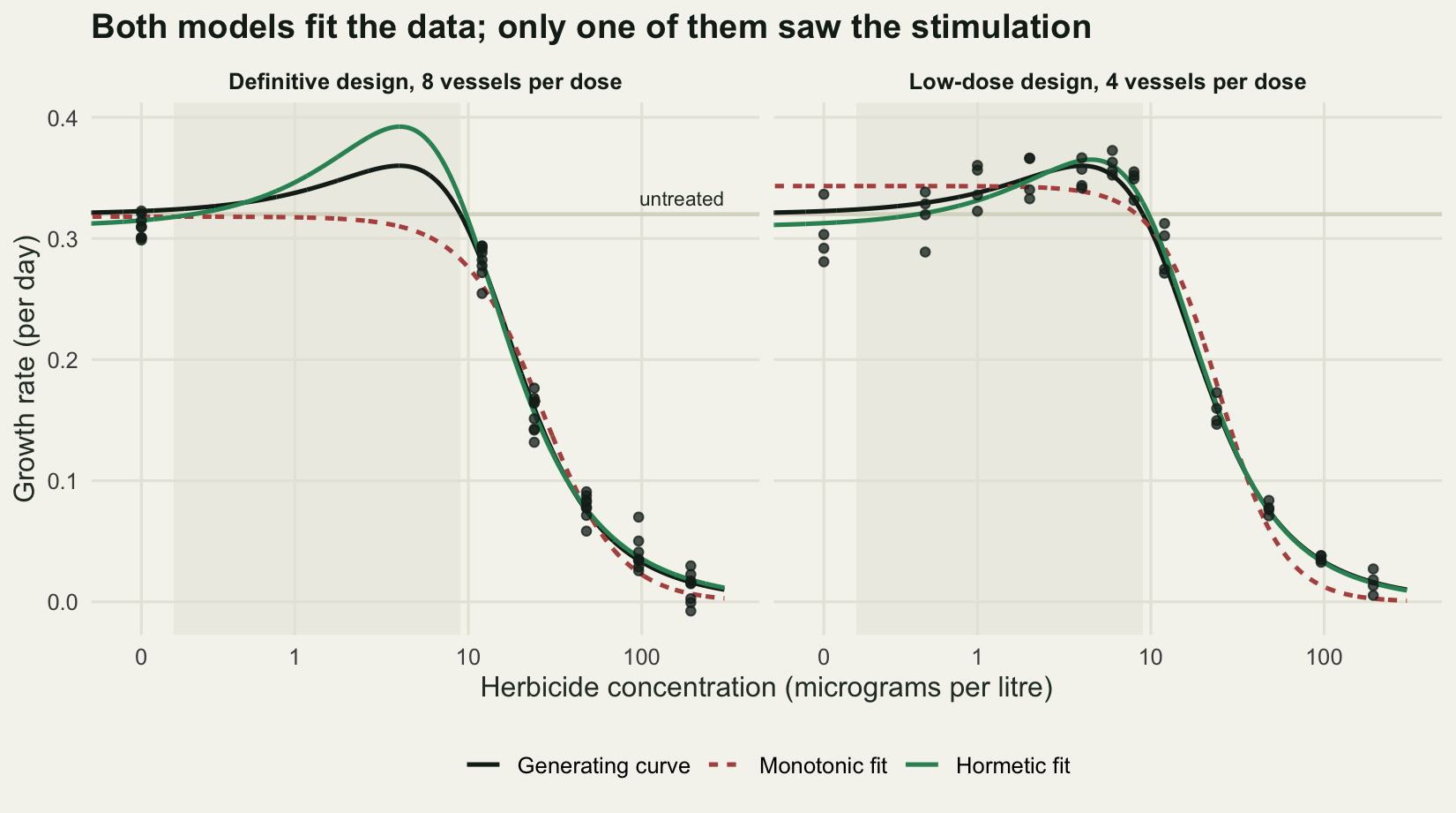

Figure 1: One simulated dataset from each of two designs, with the generating curve and the two fitted curves. The untreated vessels are drawn at the left-hand tick, and the horizontal grey line marks the untreated growth rate, labelled in the left panel. The definitive design has nothing below the dose at which the true curve returns to the untreated level, so the shaded stimulation window is empty in the left panel.

The right-hand panel shows what the low-dose design buys. Six of its twelve concentrations sit in the stimulation window, the rise is visible in the raw points, and the monotonic curve has to run through them flat and too high in order to stay decreasing. That is where the bias in the monotonic fit comes from, and the next section measures it properly instead of eyeballing one dataset.

What a monotonic fit does to the effective dose

One dataset is an anecdote. The block below simulates 500 datasets for each combination of three designs and four levels of the hormesis parameter, fits both models to each, and records the effective doses, the likelihood ratio statistic, and two empirical summaries of the raw group means. It is the only expensive block in the post and everything after it reads from the result.

The empirical summaries deserve a definition. The first records whether any treated group mean exceeded the untreated group mean, which is what somebody scanning the raw table would call a sign of stimulation. The second is a formal version of the same thing: the strongest one-sided contrast of any treated group against the untreated group, using the pooled within-group standard deviation, tested at the 0.05 level with a Bonferroni correction for the number of concentrations.

stim_test <- function(x, y) {
  lv <- sort(unique(x)); k <- length(lv); fx <- factor(x, lv)
  m <- tapply(y, fx, mean); n <- tapply(y, fx, length)
  ss <- sum(tapply(y, fx, function(z) sum((z - mean(z))^2)))
  df <- length(y) - k; s <- sqrt(ss / df)
  tt <- (m[-1] - m[1]) / (s * sqrt(1 / n[-1] + 1 / n[1]))
  c(rise = as.numeric(max(m[-1] - m[1]) > 0),
    sig = as.numeric(max(tt) > qt(1 - 0.05 / (k - 1), df)))
}

one_sim <- function(x, h_true) {
  y <- bc_mean(x, d_t, h_true, b_t, e_t) + rnorm(length(x), 0, sig)
  fm <- fit_dr(x, y, FALSE); fh <- fit_dr(x, y, TRUE); st <- stim_test(x, y)
  c(ed50_m = ed_at(50, fm[1], 0, fm[3], fm[4]),
    ed10_m = ed_at(10, fm[1], 0, fm[3], fm[4]),
    ed50_h = ed_at(50, fh[1], fh[2], fh[3], fh[4]),
    ed10_h = ed_at(10, fh[1], fh[2], fh[3], fh[4]),
    abs50_m = ed_at(NA, fm[1], 0, fm[3], fm[4], level = d_t * 0.5),
    abs10_m = ed_at(NA, fm[1], 0, fm[3], fm[4], level = d_t * 0.9),
    ctrl_m = fm[1], ctrl_h = fh[1], h_hat = fh[2],
    lrt = length(y) * log(fm[5] / fh[5]),
    peak = peak_pct(fh[1], fh[2], fh[3], fh[4]),
    rise = st[[1]], sig = st[[2]])
}

set.seed(20260731)
n_sim <- 500
h_grid <- c(0, 0.005, 0.01, 0.02)
sims <- list()
for (dn in names(designs)) for (hh in h_grid)
  sims[[paste(dn, hh)]] <- t(replicate(n_sim, one_sim(designs[[dn]], hh)))
c(datasets_per_cell = n_sim, cells = length(sims),
  fits = 2 * n_sim * length(sims),
  failed_ED_values = sum(sapply(sims, function(z) sum(is.na(z)))))

datasets_per_cell             cells              fits  failed_ED_values 
              500                12             12000                 7 

Across all 12000 fits, 7 effective doses could not be computed, all of them from hormetic fits whose estimated curve never reaches the target level. Those are dropped from the medians below and counted rather than hidden.

tr <- c(ED50 = ed_at(50, d_t, h_t, b_t, e_t), ED10 = ed_at(10, d_t, h_t, b_t, e_t))
med <- function(z) median(z, na.rm = TRUE)

bias_tab <- t(sapply(names(designs), function(dn) {
  r <- sims[[paste(dn, h_t)]]
  c(ED50_monotonic = med(r[, "ed50_m"]), ED50_hormetic = med(r[, "ed50_h"]),
    ED10_monotonic = med(r[, "ed10_m"]), ED10_hormetic = med(r[, "ed10_h"]))
}))
print(round(bias_tab, 3))

           ED50_monotonic ED50_hormetic ED10_monotonic ED10_hormetic
definitive         25.622        24.008          8.298        11.427
extended           23.881        24.032          8.036        11.431
low_dose           24.497        24.026          8.964        11.390

print(round(100 * (sweep(bias_tab, 2, tr[c(1, 1, 2, 2)], "/") - 1), 2))

           ED50_monotonic ED50_hormetic ED10_monotonic ED10_hormetic
definitive           6.76          0.03         -27.23          0.21
extended            -0.50          0.13         -29.53          0.25
low_dose             2.07          0.11         -21.39         -0.12

decomp <- t(sapply(names(designs), function(dn) {
  r <- sims[[paste(dn, h_t)]]
  unname(c(control_monotonic = med(r[, "ctrl_m"]),
           control_hormetic = med(r[, "ctrl_h"]),
           control_bias_pct = 100 * (med(r[, "ctrl_m"]) / d_t - 1),
           ED50_fixed_level_bias_pct = 100 * (med(r[, "abs50_m"]) / tr["ED50"] - 1),
           ED10_fixed_level_bias_pct = 100 * (med(r[, "abs10_m"]) / tr["ED10"] - 1)))
}))
colnames(decomp) <- c("control_monotonic", "control_hormetic", "control_bias_pct",
                      "ED50_fixed_level_bias_pct", "ED10_fixed_level_bias_pct")
print(round(decomp, 4))

           control_monotonic control_hormetic control_bias_pct
definitive            0.3257           0.3197           1.7700
extended              0.3495           0.3196           9.2296
low_dose              0.3459           0.3204           8.1049
           ED50_fixed_level_bias_pct ED10_fixed_level_bias_pct
definitive                    8.8332                  -21.2142
extended                      8.1729                   -2.0640
low_dose                      9.1848                    3.2351

The hormetic model recovers both quantities on all three designs, within 0.25 per cent of the truth at the median, which is the calibration the rest of the section is measured against. The monotonic model does something more interesting than being uniformly wrong.

Its ED50 is almost right: 6.76 per cent high on the definitive design, 0.5 per cent low on the extended design, 2.07 per cent high on the low-dose design. A laboratory comparing monotonic ED50 values between runs would see nothing at all. Its ED10, on the same fits, is 27.23, 29.53 and 21.39 per cent low. The bias is severe, it is in the same direction on every design, and it points downward, so the monotonic model reports a more protective number than the truth. That was not the direction I expected before running it, and the reason is visible in the decomposition.

The monotonic fit has to explain observations that lie above the untreated level, and the only parameter it has for the job is the upper plateau. On the extended design it estimates the untreated growth rate at 0.3495 instead of 0.32, 9.23 per cent too high. Everything downstream is then measured against a ceiling that the untreated vessels never reached. Recompute the same monotonic fits with the target response level fixed at the true untreated rate instead of the fitted one, and the ED10 bias on the extended design falls from 29.53 per cent to 2.06 per cent, while the ED50 bias moves the other way, from 0.5 per cent low to 8.17 per cent high. So the ED50 looked fine by cancellation: the fitted curve sits too high, and the fitted ceiling sits too high by about the same amount, and at the halfway point the two errors nearly cancel. At the ten per cent level they do not, because a ten per cent drop from an inflated ceiling is reached much earlier on the dose axis.

des_lab <- c(definitive = "Definitive", extended = "Extended", low_dose = "Low dose")
box_df <- do.call(rbind, lapply(names(designs), function(dn) {
  r <- sims[[paste(dn, h_t)]]
  data.frame(design = factor(des_lab[[dn]], levels = unname(des_lab)),
             model = factor(rep(c("Monotonic", "Hormetic"), each = nrow(r)),
                            levels = c("Monotonic", "Hormetic")),
             value = c(r[, "ed10_m"], r[, "ed10_h"]),
             level = "ED10 (micrograms per litre)")
}))
box_df <- rbind(box_df, do.call(rbind, lapply(names(designs), function(dn) {
  r <- sims[[paste(dn, h_t)]]
  data.frame(design = factor(des_lab[[dn]], levels = unname(des_lab)),
             model = factor(rep(c("Monotonic", "Hormetic"), each = nrow(r)),
                            levels = c("Monotonic", "Hormetic")),
             value = c(r[, "ed50_m"], r[, "ed50_h"]),
             level = "ED50 (micrograms per litre)")
})))
box_df <- box_df[!is.na(box_df$value), ]
ref <- data.frame(level = c("ED10 (micrograms per litre)", "ED50 (micrograms per litre)"),
                  y = as.numeric(tr[c("ED10", "ED50")]))

ggplot(box_df, aes(design, value, fill = model)) +
  geom_hline(data = ref, aes(yintercept = y), colour = te_pal$clay, linewidth = 0.8) +
  stat_summary(fun.data = function(z)
    data.frame(ymin = quantile(z, 0.05), lower = quantile(z, 0.25),
               middle = median(z), upper = quantile(z, 0.75),
               ymax = quantile(z, 0.95)),
    geom = "boxplot", position = position_dodge(width = 0.72), width = 0.62,
    colour = te_pal$ink, linewidth = 0.4) +
  facet_wrap(~level, scales = "free_y") +
  scale_fill_manual(values = c(Monotonic = te_pal$sage, Hormetic = te_pal$green),
                    name = NULL) +
  labs(x = NULL, y = "Estimated effective dose",
       title = "The monotonic fit misses the ED10 by far more than it misses the ED50") +
  theme_te() +
  theme(legend.position = "bottom",
        strip.text = element_text(colour = te_pal$ink, face = "bold"))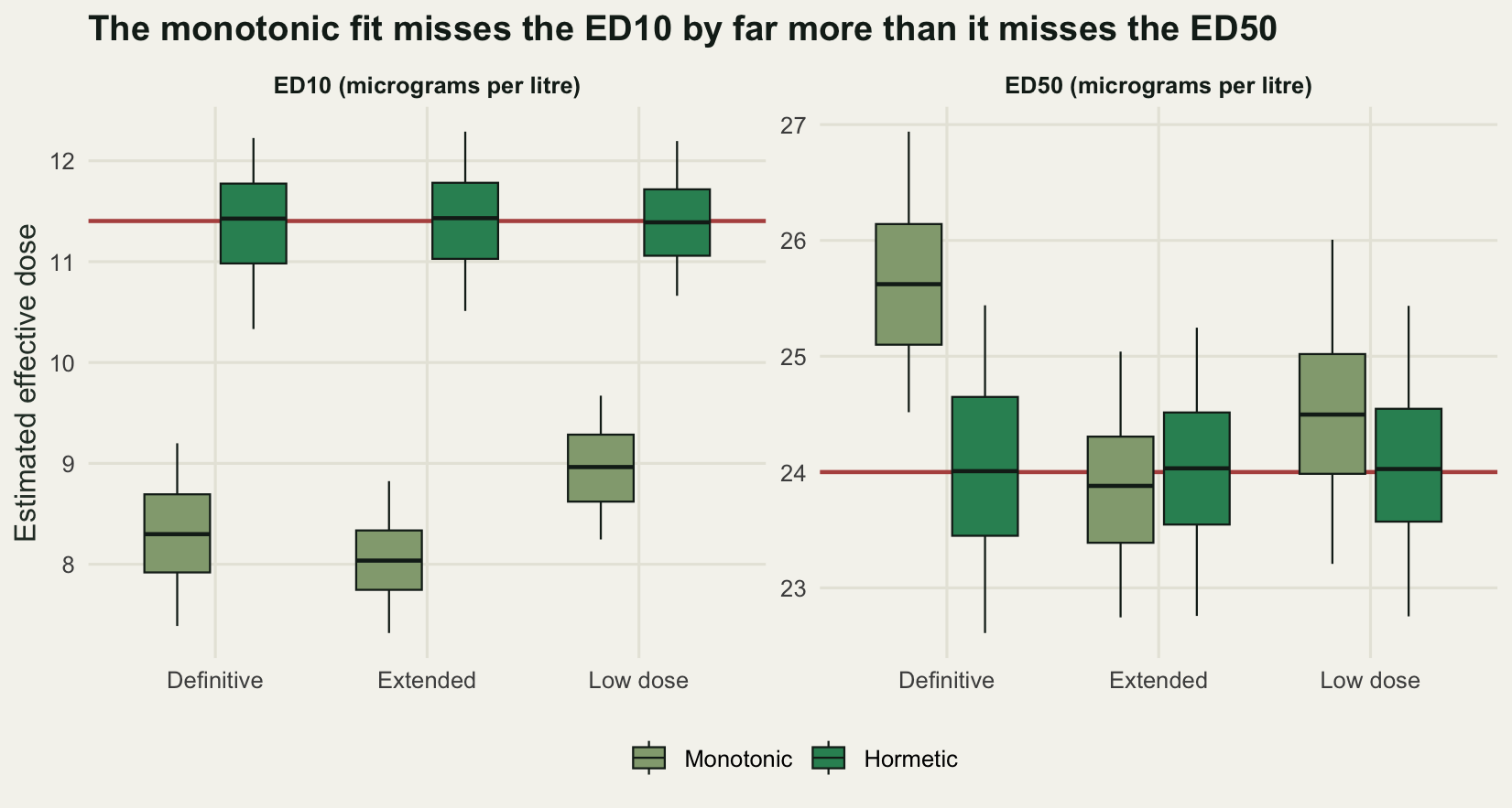

Figure 2: Sampling distributions of the two effective doses over 500 simulated datasets per design, with the hormesis parameter at its true value. The horizontal line in each panel is the value in the generating curve. Boxes show the median and quartiles, whiskers the 5th and 95th percentiles.

What the extra parameter costs when there is nothing to find

A model that only helps when the phenomenon is present is not much use, because the decision to use it has to be made before anyone knows. The calibration row is the one where the generating curve has no hormesis at all: the same 500 datasets per design, simulated with the hormesis parameter set to zero, fitted with both models.

cat("median estimated hormesis parameter with no hormesis present:\n")

median estimated hormesis parameter with no hormesis present:

for (dn in names(designs))
  cat(sprintf("  %-11s %.6f\n", dn, med(sims[[paste(dn, 0)]][, "h_hat"])))

  definitive  0.000259
  extended    0.000050
  low_dose    0.000293

calib <- t(sapply(names(designs), function(dn) {
  r <- sims[[paste(dn, 0)]]
  c(ED50_monotonic = med(r[, "ed50_m"]), ED50_hormetic = med(r[, "ed50_h"]),
    ED10_monotonic = med(r[, "ed10_m"]), ED10_hormetic = med(r[, "ed10_h"]),
    test_size = mean(r[, "lrt"] > qchisq(0.95, 1)))
}))
print(round(calib, 4))

           ED50_monotonic ED50_hormetic ED10_monotonic ED10_hormetic test_size
definitive        11.9891       11.9934         3.9966        4.0422     0.034
extended          12.0314       12.0021         4.0000        4.0213     0.066
low_dose          11.9911       11.9814         3.9974        4.0186     0.084

price <- t(sapply(names(designs), function(dn) {
  r <- sims[[paste(dn, 0)]]
  c(iqr_ED50_monotonic = IQR(r[, "ed50_m"], na.rm = TRUE),
    iqr_ED50_hormetic = IQR(r[, "ed50_h"], na.rm = TRUE),
    iqr_ED10_monotonic = IQR(r[, "ed10_m"], na.rm = TRUE),
    iqr_ED10_hormetic = IQR(r[, "ed10_h"], na.rm = TRUE))
}))
print(round(cbind(price,
                  ED50_width_ratio = price[, 2] / price[, 1],
                  ED10_width_ratio = price[, 4] / price[, 3]), 3))

           iqr_ED50_monotonic iqr_ED50_hormetic iqr_ED10_monotonic
definitive              0.568             0.551              0.549
extended                0.579             0.601              0.434
low_dose                0.550             0.561              0.426
           iqr_ED10_hormetic ED50_width_ratio ED10_width_ratio
definitive             2.040            0.971            3.715
extended               0.643            1.039            1.482
low_dose               0.600            1.021            1.409

Nothing goes wrong with the point estimates. The median estimated hormesis parameter is 0.000259, 0.000050 and 0.000293 on the three designs against a true zero. On the definitive design the monotonic ED50 median is 11.9891 and the hormetic one 11.9934, against a true 12; the two ED10 medians are 3.9966 and 4.0422, against a true 4. The likelihood ratio test rejects at rates of 0.034, 0.066 and 0.084 against a nominal 0.05, so the reference distribution is usable, with the low-dose design a little liberal.

The price is paid in precision, and only in one place. The interquartile range of the ED50 is essentially unchanged: the ratio of hormetic to monotonic width is 0.971, 1.039 and 1.021. The interquartile range of the ED10 is a different matter. On the extended and low-dose designs the extra parameter widens it by a factor of 1.482 and 1.409, which is a real cost but a payable one. On the definitive design the factor is 3.715. Adding a parameter that describes the shape of the curve below the lowest tested concentration, on a design with no data below the lowest tested concentration, spreads the ED10 out by nearly four times and buys nothing when the curve is monotonic.

That is the answer to whether the extension is safe to apply routinely. On a design that covers the stimulation range it is close to free. On the design most laboratories actually run it is expensive, and the expense falls exactly on the quantity the extension was supposed to protect.

What a test for hormesis actually tests

Now the power question, and it is where the post stopped agreeing with what I assumed when I started. Two tests are recorded for every dataset. The likelihood ratio test asks whether the hormesis parameter differs from zero. The corrected dose contrast asks whether any treated group grew faster than the untreated group. They are usually described as two routes to the same conclusion.

pow <- do.call(rbind, lapply(names(designs), function(dn)
  t(sapply(h_grid, function(hh) {
    r <- sims[[paste(dn, hh)]]
    c(h = hh, true_peak_pct = peak_pct(d_t, hh, b_t, e_t),
      lrt_power = mean(r[, "lrt"] > qchisq(0.95, 1)),
      any_group_above_control = mean(r[, "rise"]),
      contrast_power = mean(r[, "sig"]))
  }))))
pow <- data.frame(design = rep(unname(des_lab), each = length(h_grid)), pow)
print(round(pow[, -1], 4))

       h true_peak_pct lrt_power any_group_above_control contrast_power
1  0.000        0.0000     0.034                   0.000          0.000
2  0.005        0.8713     0.160                   0.000          0.000
3  0.010        3.3999     0.496                   0.000          0.000
4  0.020       12.5000     0.998                   0.000          0.000
5  0.000        0.0000     0.066                   0.012          0.000
6  0.005        0.8713     0.442                   0.276          0.002
7  0.010        3.3999     0.930                   0.874          0.056
8  0.020       12.5000     1.000                   1.000          0.976
9  0.000        0.0000     0.084                   0.666          0.008
10 0.005        0.8713     0.332                   0.820          0.012
11 0.010        3.3999     0.874                   0.942          0.070
12 0.020       12.5000     1.000                   1.000          0.884

spread <- t(sapply(names(designs), function(dn) {
  r <- sims[[paste(dn, h_t)]]
  c(median_peak_pct = med(r[, "peak"]),
    q05 = quantile(r[, "peak"], 0.05), q95 = quantile(r[, "peak"], 0.95))
}))
print(round(cbind(true_peak_pct = peak_pct(d_t, h_t, b_t, e_t), spread), 2))

           true_peak_pct median_peak_pct q05.5% q95.95%
definitive          12.5           11.96   4.34   37.16
extended            12.5           12.77   8.16   17.19
low_dose            12.5           12.26   8.20   16.81

At the true hormesis level the likelihood ratio test rejects in 0.998 of definitive-design datasets. The contrast test rejects in 0.000 of them, and not a single one of the 500 datasets had even one treated group mean above the untreated mean. A test with essentially perfect power sits next to zero observations of the thing being tested. Both statements are correct. The likelihood ratio test is not a test of low-dose stimulation; it is a test of whether the descending limb has the shape the three parameter curve says it should. On the definitive design that is the only evidence available, and the model converts it into a claim about a concentration range nobody dosed.

The estimated size of the stimulation shows what that claim is worth. On the definitive design the median estimated peak is 11.96 per cent against a true 12.5, so it is not biased, but the 5th to 95th percentile range runs from 4.34 to 37.16 per cent. On the low-dose design the same range is 8.20 to 16.81. The definitive design gets the right answer on average and, in any individual run, puts the size of the stimulation inside a range that spans most of an order of magnitude.

Read the table the other way, as a design question, and the ordering changes. For the contrast test, which has to see the rise, the definitive design has no power at any hormesis level: 0.000 in all four rows. The comparison between the other two is closer than I expected and it does not go the same way at both stimulation sizes. At the true level the extended design wins, 0.976 against 0.884, because it puts six vessels on each of two concentrations inside the stimulation window rather than four vessels on each of six. One step down, at a stimulation of 3.3999 per cent, the low-dose design wins, 0.070 against 0.056, because with a rise that small it matters more that some concentration lands near the top of the bump than that any one of them is well replicated. For estimating the size of the stimulation rather than detecting it, the low-dose design is slightly ahead of the extended one on both measures already computed: an ED10 interquartile range of 0.600 against 0.643 under no hormesis, and a peak interval of 8.20 to 16.81 against 8.16 to 17.19.

test_lab <- c("Likelihood ratio test for the\nhormesis parameter",
              "Strongest dose contrast against\nthe untreated group")
pw <- rbind(data.frame(design = pow$design, x = pow$true_peak_pct,
                       y = pow$lrt_power, test = test_lab[1]),
            data.frame(design = pow$design, x = pow$true_peak_pct,
                       y = pow$contrast_power, test = test_lab[2]))
pw$test <- factor(pw$test, levels = test_lab)
pw$design <- factor(pw$design, levels = unname(des_lab))

ggplot(pw, aes(x, y, colour = design, group = design)) +
  geom_hline(yintercept = 0.05, colour = te_pal$line, linewidth = 0.8) +
  geom_line(linewidth = 0.9) +
  geom_point(size = 2.4) +
  facet_wrap(~test) +
  scale_y_continuous(limits = c(0, 1)) +
  scale_colour_manual(values = c(Definitive = te_pal$clay, Extended = te_pal$gold,
                                 `Low dose` = te_pal$forest), name = NULL) +
  labs(x = "Stimulation in the generating curve (per cent above the untreated level)",
       y = "Rejection rate",
       title = "One test needs to see the rise and the other one does not") +
  theme_te() +
  theme(legend.position = "bottom",
        strip.text = element_text(colour = te_pal$ink, face = "bold"))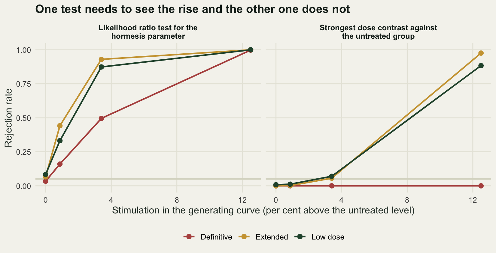

Figure 3: Rejection rate of two tests over 500 datasets per point, against the size of the stimulation in the generating curve. The left panel tests the hormesis parameter inside the fitted curve; the right panel tests whether any treated group grew faster than the untreated group. The horizontal line is the nominal 0.05 level.

The number that reaches the risk assessment

Suppose the regulatory endpoint is the ED10, which is common for growth endpoints. The two models were fitted to the same vessels, and the difference between them is what the risk assessment inherits.

gap <- t(sapply(names(designs), function(dn) {
  r <- sims[[paste(dn, h_t)]]
  g <- 100 * (r[, "ed10_m"] / r[, "ed10_h"] - 1)
  c(ED10_monotonic = med(r[, "ed10_m"]), ED10_hormetic = med(r[, "ed10_h"]),
    pct_difference = med(g),
    q05 = quantile(g, 0.05, na.rm = TRUE), q95 = quantile(g, 0.95, na.rm = TRUE),
    share_below = mean(g < 0, na.rm = TRUE))
}))
print(round(gap, 3))

           ED10_monotonic ED10_hormetic pct_difference  q05.5% q95.95%
definitive          8.298        11.427        -27.093 -33.077 -20.472
extended            8.036        11.431        -29.713 -32.944 -25.890
low_dose            8.964        11.390        -21.331 -24.770 -17.915
           share_below
definitive           1
extended             1
low_dose             1

On the definitive design the monotonic ED10 is 27.1 per cent below the hormetic one at the median, and it is below it in 1.000 of the 500 datasets, with a 5th to 95th percentile range of 33.1 to 20.5 per cent below. The direction never changes. The monotonic model is not adding noise to the regulatory number, it is shifting it, and the shift survives replication of the whole experiment.

Two consequences follow, and they point opposite ways. The monotonic ED10 is the more protective number, so nothing bad happens to the organisms if the analysis is wrong in this direction. But the ED10 is a quantity that gets compared: against measured environmental concentrations, against values for other substances, and against the same substance tested in another laboratory with a different concentration series. The size of the shift depends on the design, at 27.23, 29.53 and 21.39 per cent low on the three designs here, so two laboratories fitting monotonic curves to hormetic data will disagree by an amount that has nothing to do with the chemical. That is the part worth telling the assessor about.

The honest limit

A hormetic curve shape is not evidence of a hormetic mechanism, and the machinery above cannot tell the difference. The standard alternative explanations are a mixed population, in which a tolerant subgroup keeps growing while a sensitive subgroup is knocked out, and exposure that is not constant over the test. The mixture case is easy to simulate, so it gets measured rather than asserted: two subpopulations in equal proportions, each with a monotonic log-logistic response, one with its curve parameter at 8 and the other at 60, and the vessel-level measurement is their average.

mix_mean <- function(x, d, b, e1, e2, w = 0.5)
  d * (w / (1 + exp(b * (log(x) - log(e1)))) +
       (1 - w) / (1 + exp(b * (log(x) - log(e2)))))

e1 <- 8; e2 <- 60; b_mix <- 3
f_mix <- mix_mean(grid_x, d_t, b_mix, e1, e2)
mix_ed <- function(p) uniroot(function(z)
  mix_mean(z, d_t, b_mix, e1, e2) - d_t * (1 - p / 100), c(0.05, 300))$root
round(c(sensitive_e = e1, tolerant_e = e2, max_over_control_ratio = max(f_mix) / d_t,
        mixture_ED10 = mix_ed(10), mixture_ED50 = mix_ed(50)), 4)

           sensitive_e             tolerant_e max_over_control_ratio 
                8.0000                60.0000                 1.0000 
          mixture_ED10           mixture_ED50 
                5.0335                21.9089 

set.seed(20260731)
n_mix <- 400
mix_run <- function(x) {
  y <- mix_mean(x, d_t, b_mix, e1, e2) + rnorm(length(x), 0, sig)
  fm <- fit_dr(x, y, FALSE); fh <- fit_dr(x, y, TRUE); st <- stim_test(x, y)
  c(lrt = length(y) * log(fm[5] / fh[5]), h_hat = fh[2],
    peak = peak_pct(fh[1], fh[2], fh[3], fh[4]),
    ed10_m = ed_at(10, fm[1], 0, fm[3], fm[4]),
    ed10_h = ed_at(10, fh[1], fh[2], fh[3], fh[4]),
    rise = st[[1]], sig = st[[2]])
}
mix_res <- lapply(designs[c("definitive", "low_dose")], function(x)
  t(replicate(n_mix, mix_run(x))))
print(round(t(sapply(mix_res, function(r) c(
  lrt_rejection_rate = mean(r[, "lrt"] > qchisq(0.95, 1)),
  median_h_hat = med(r[, "h_hat"]), share_h_positive = mean(r[, "h_hat"] > 0),
  median_fitted_peak_pct = med(r[, "peak"]),
  contrast_rejection = mean(r[, "sig"]),
  ED10_monotonic = med(r[, "ed10_m"]), ED10_hormetic = med(r[, "ed10_h"]),
  ED10_monotonic_pct_error = 100 * (med(r[, "ed10_m"]) / mix_ed(10) - 1),
  ED10_hormetic_pct_error = 100 * (med(r[, "ed10_h"]) / mix_ed(10) - 1)))), 4))

           lrt_rejection_rate median_h_hat share_h_positive
definitive              1.000      -0.0017           0.0000
low_dose                0.425      -0.0014           0.0375
           median_fitted_peak_pct contrast_rejection ED10_monotonic
definitive                -0.2044             0.0000         3.2395
low_dose                  -0.0237             0.0075         3.4757
           ED10_hormetic ED10_monotonic_pct_error ED10_hormetic_pct_error
definitive        1.5879                 -35.6413                -68.4524
low_dose          2.9280                 -30.9491                -41.8305

no_horm <- sims[["low_dose 0"]]
round(c(any_group_above_control = mean(no_horm[, "rise"]),
        corrected_contrast_rejects = mean(no_horm[, "sig"]),
        median_fitted_peak_pct = med(no_horm[, "peak"])), 4)

   any_group_above_control corrected_contrast_rejects 
                    0.6660                     0.0080 
    median_fitted_peak_pct 
                    0.0025 

The mixture never rises above the untreated level: its maximum is 1.0000 times the untreated value, attained at zero dose. It contains no stimulation of any kind. Yet the likelihood ratio test for the hormesis parameter rejects in 1.000 of definitive-design datasets and 0.425 of low-dose-design datasets. The saving grace is the sign. The estimated hormesis parameter is negative in almost every fit, positive in 0.000 of the definitive-design fits and 0.0375 of the low-dose ones, and the fitted peak sits 0.2044 per cent below the untreated level rather than above it. So the test is detecting that a three parameter log-logistic curve is the wrong shape, which is true, and the extra parameter is being spent on something other than hormesis.

The damage lands on the ED10 again, and this time the extension makes it worse. The true mixture ED10 is 5.03. The monotonic fit gives 3.24 on the definitive design, 35.6 per cent low. The hormetic fit gives 1.59, 68.5 per cent low, because it has been handed a parameter with which to curve the low-dose region and no data to constrain it. Fitting the more flexible model when the shape is wrong for a different reason does not help.

The failure runs the other way as well. On the low-dose design with a genuinely monotonic generating curve, at least one treated group mean exceeded the untreated mean in 0.666 of the 500 datasets. Two runs in three would show a technician something that looks like stimulation in the raw table, with no stimulation anywhere in the generating model. The corrected contrast rejected in 0.008 of them, which is the whole argument for using it: the eye finds low-dose stimulation roughly two thirds of the time in data that contains none, and the corrected test finds it in under one per cent.

set.seed(9081)
xm <- designs$low_dose
ym <- mix_mean(xm, d_t, b_mix, e1, e2) + rnorm(length(xm), 0, sig)
fh_mix <- fit_dr(xm, ym, TRUE)
mix_lab <- c("Sensitive subpopulation", "Tolerant subpopulation",
             "Mixture (the truth)", "Hormetic model fitted to the mixture")
mix_df <- data.frame(
  dose = rep(grid_x, 4),
  y = c(d_t / (1 + exp(b_mix * (log(grid_x) - log(e1)))),
        d_t / (1 + exp(b_mix * (log(grid_x) - log(e2)))),
        f_mix, bc_mean(grid_x, fh_mix[1], fh_mix[2], fh_mix[3], fh_mix[4])),
  kind = factor(rep(mix_lab, each = length(grid_x)), levels = mix_lab))
mix_pts <- data.frame(dose = ifelse(xm == 0, pseudo0, xm), y = ym)

ggplot(mix_df, aes(dose, y, colour = kind, linewidth = kind, linetype = kind)) +
  geom_hline(yintercept = d_t, colour = te_pal$line, linewidth = 0.8) +
  geom_line() +
  geom_point(data = mix_pts, aes(dose, y), inherit.aes = FALSE,
             colour = te_pal$ink, size = 1.5, alpha = 0.75) +
  scale_x_log10(breaks = c(pseudo0, 1, 10, 100), labels = c("0", "1", "10", "100")) +
  coord_cartesian(xlim = c(0.1, 320)) +
  scale_colour_manual(values = c("#5d7a49", te_pal$gold, te_pal$ink, te_pal$clay),
                      name = NULL) +
  scale_linewidth_manual(values = c(0.9, 0.9, 1.2, 1.0), name = NULL) +
  scale_linetype_manual(values = c("solid", "solid", "solid", "22"), name = NULL) +
  labs(x = "Herbicide concentration (micrograms per litre)",
       y = "Growth rate (per day)",
       title = "The hormetic curve fits a mixture that never rises above the untreated level") +
  theme_te() +
  theme(legend.position = "bottom") +
  guides(colour = guide_legend(nrow = 2))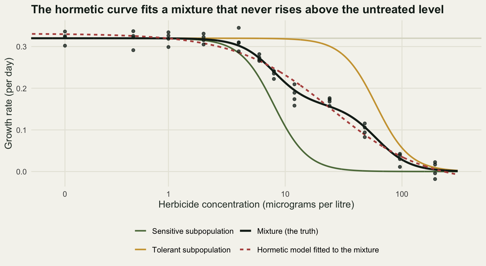

Figure 4: A mixture of two sensitivities, with the fitted hormetic curve from one simulated dataset on the low-dose design. The mixture is monotonic by construction and never exceeds the untreated level, but the three parameter log-logistic shape is wrong for it, and the extra parameter takes a negative value rather than a hormetic one.

Three further limits are worth stating plainly. The lower asymptote was fixed at zero throughout; estimating it instead adds a fifth parameter that competes with the hormesis term for the same information, and the ED10 spread measured above would grow further. The residual variance was constant on the growth rate scale, whereas real growth data are usually more variable at intermediate concentrations, which is the subject of checking a bounded-response model. And the whole exercise assumed the concentration on the label is the concentration in the vessel; herbicides adsorb and degrade over seven days, and that is a different bias with a different sign.

Where to go next

The practical recommendation from all of this is a design one rather than a modelling one. If the ED10 is the number that matters, spend part of the vessel budget below the lowest concentration that a range-finder says does anything, because that is where the untreated level and the shape of the low-dose region are decided, and no choice of curve family recovers what the design did not measure. Two extra concentrations with full replication did more here than six with a quarter of it.

Checking a dose-response analysis works through the other ways the same fit goes wrong, including control mortality, overdispersion between vessels, and extrapolation below the lowest tested dose, which is what the ED10 estimates in the definitive design above really are. If the low-dose region turns out to have a threshold rather than a bump, segmented regression and breakpoints fits that shape instead and gives a confidence interval for where the response starts.

References

Brain P, Cousens R 1989 Weed Research 29(2):93-96 (10.1111/j.1365-3180.1989.tb00845.x)

Calabrese EJ, Baldwin LA 2003 Nature 421(6924):691-692 (10.1038/421691a)

Cedergreen N, Ritz C, Streibig JC 2005 Environmental Toxicology and Chemistry 24(12):3166-3172 (10.1897/05-014R.1)

Ritz C 2010 Environmental Toxicology and Chemistry 29(1):220-229 (10.1002/etc.7)

Ritz C, Baty F, Streibig JC, Gerhard D 2015 PLOS ONE 10(12):e0146021 (10.1371/journal.pone.0146021)

Related tutorials

• Dose-response curves and the LC50
• Segmented regression and breakpoints
• Nonlinear regression with nls
• Checking a dose-response analysis