library(ggplot2)
library(patchwork)

te_paper  <- "#f5f4ee"
te_ink    <- "#16241d"
te_body   <- "#2c3a31"
te_forest <- "#275139"
te_rust   <- "#b5534e"
te_gold   <- "#c9b458"
te_line   <- "#dad9ca"

theme_datasheet <- function() {
  theme_minimal(base_size = 12) +
    theme(plot.background  = element_rect(fill = te_paper, colour = NA),
          panel.background = element_rect(fill = te_paper, colour = NA),
          panel.grid.major = element_line(colour = te_line, linewidth = 0.3),
          panel.grid.minor = element_blank(),
          text             = element_text(colour = te_body),
          plot.title       = element_text(colour = te_ink, face = "bold"),
          plot.subtitle    = element_text(colour = te_body),
          axis.text        = element_text(colour = te_body),
          strip.text       = element_text(colour = te_ink, face = "bold"))
}Trawl selectivity when hauls differ
R
fisheries
selectivity
GLM
overdispersion
simulation
ecology tutorial
Pooling covered-codend hauls into one logistic selectivity curve gives an L50 interval that misses. Why quasi-binomial fails in R, and why the haul is the unit.
A research vessel tows a bottom trawl with a fine-meshed cover laced over the codend. Every fish that escapes through the codend meshes is caught in the cover, so after each haul the catch splits into two piles, measured to the centimetre: fish retained by the codend and fish that got through. Twelve hauls later there is a table of retained and total counts by length, and the number the gear trial exists for is the L50, the length at which a fish has an even chance of being retained, together with the selection range, the distance between the lengths retained with probabilities of one quarter and three quarters.
The usual first analysis adds the twelve hauls together length by length and fits one logistic curve. It gives a sharp curve and a narrow interval, because it has several thousand fish behind it. It also assumes that all twelve hauls share one curve. They do not. Tow duration, catch volume in the codend, sea state and the species mix can all move the curve from haul to haul, and Fryer 1991 built a model of exactly that between-haul variation. This post demonstrates that known result rather than discovering it: with haul-to-haul variation in L50 of a centimetre, the pooled interval covers the true mean L50 in fewer than half of the simulated trials.
The more useful part is why the standard repair does not work. The post on checking a dose-response analysis meets the same problem in a toxicity test, where animals share a vessel, and there a quasi-binomial dispersion estimate brings coverage back close to nominal. That works because each vessel is one cell of the data: the vessel effect shows up as extra scatter in that cell’s count, and the Pearson statistic can see it. A haul is not one cell. Its shift moves the whole curve, and it is spread over thirty length classes, most of which sit at a retention near zero or one where a shift of a centimetre changes almost nothing. The dispersion statistic rises a little while the design effect for L50 grows many times over. Pseudoreplication with nested counts shows the generic version of the overconfident pooled GLM with a random intercept as the repair; here the grouping acts on a curve parameter, and the repair has to act on that parameter too. The logistic curve itself, and the delta-method interval for the length at fifty per cent, are the same machinery as the LC50 in dose-response curves and the LC50, with length in place of log concentration.
Twelve hauls, twelve curves
The simulation fixes the design before any coverage is inspected. Lengths run from 10 to 40 cm, the true mean L50 is 25 cm and the selection range is 4 cm, which on the logit scale is a slope of two times log three divided by the selection range. Each haul gets its own L50, drawn from a normal distribution around 25 cm, and its own catch size: the expected number of fish per length class in a haul is drawn from a gamma distribution with mean 20 and shape 4, so some hauls bring in a few hundred fish and some well over a thousand. Retained counts are binomial given the haul’s curve. Every coverage figure below uses 300 simulated datasets per setting.
len_cm     <- 10:40          # length classes, cm
l50_true   <- 25             # mean L50 over hauls, cm
sr_true    <- 4              # selection range, cm
b_true     <- 2 * log(3) / sr_true
fish_mean  <- 20             # expected fish per length class per haul
fish_shape <- 4              # gamma shape for haul-to-haul catch size
n_rep      <- 300            # datasets per setting, fixed in advance
n_len      <- length(len_cm)
fam_bin    <- binomial()

sim_hauls <- function(H, sd_haul, fish = fish_mean, rho_cell = 0) {
  l50_h <- l50_true + rnorm(H, 0, sd_haul)
  lam_h <- rgamma(H, fish_shape, fish_shape / fish)
  n_mat <- matrix(rpois(H * n_len, rep(lam_h, each = n_len)), nrow = n_len)
  p_mat <- matrix(plogis(b_true * (len_cm - rep(l50_h, each = n_len))), nrow = n_len)
  if (rho_cell > 0) {          # cell-level beta-binomial noise, used later
    s_bb  <- (1 - rho_cell) / rho_cell
    p_mat <- matrix(rbeta(H * n_len, p_mat * s_bb, (1 - p_mat) * s_bb), nrow = n_len)
  }
  r_mat <- matrix(rbinom(H * n_len, n_mat, p_mat), nrow = n_len)
  list(n = n_mat, r = r_mat, l50_h = l50_h, H = H)
}
Three fits come out of one function. It fits a binomial logistic regression by iteratively reweighted least squares, returns L50 as minus the intercept over the slope with its delta-method standard error, and returns the Pearson chi-squared statistic and its degrees of freedom so the dispersion can be estimated. It also flags a fit that did not converge or came back with a slope that is not positive, which happens with sparse hauls, and returns the residual deviance and the Wald statistic of the slope, which are used later to find fits that report convergence but carry no usable L50.
fit_logit <- function(x, r, n) {
  keep <- n > 0
  xm <- cbind(1, x[keep]); rk <- r[keep]; nk <- n[keep]
  f  <- suppressWarnings(glm.fit(xm, cbind(rk, nk - rk), family = fam_bin))
  co <- f$coefficients; mu <- f$fitted.values
  wt <- nk * mu * (1 - mu)
  vc <- tryCatch(solve(crossprod(xm * sqrt(wt))), error = function(e) matrix(NA, 2, 2))
  grad <- c(-1 / co[2], co[1] / co[2]^2)
  c(l50 = unname(-co[1] / co[2]),
    se  = sqrt(max(0, drop(grad %*% vc %*% grad))),
    x2  = sum((rk - nk * mu)^2 / wt), df = sum(keep) - 2,
    ok  = as.numeric(f$converged && co[2] > 0),
    dev = f$deviance, zb = unname(co[2] / sqrt(vc[2, 2])))
}

# random-L50 model: per-haul estimates y with known variances v, REML for tau2
reml_l50 <- function(y, v) {
  nll <- function(lt) {
    w <- 1 / (v + exp(lt)); m <- sum(w * y) / sum(w)
    0.5 * (sum(log(v + exp(lt))) + log(sum(w)) + sum(w * (y - m)^2))
  }
  tau2 <- exp(optimize(nll, c(-12, 5), tol = 1e-8)$minimum)
  w <- 1 / (v + tau2)
  c(mu = sum(w * y) / sum(w), se = sqrt(1 / sum(w)), tau2 = tau2)
}
The last function is a one-parameter version of Fryer’s model. Each haul’s L50 estimate is treated as the haul’s true L50 plus estimation error with its own known variance, and the true L50s scatter around a mean with a between-haul variance that is estimated by restricted maximum likelihood. The mean is then a weighted average in which a haul counts for less when its own estimate is poor or when the between-haul variance dominates. Fryer’s version carries both curve parameters of each haul together, with a two by two between-haul covariance matrix; the one-parameter reduction is enough for an interval on L50.
set.seed(4107)
ex_h <- 12; ex_sd <- 1
ex <- sim_hauls(ex_h, ex_sd)
ex_pool <- fit_logit(rep(len_cm, ex_h), as.vector(ex$r), as.vector(ex$n))
ex_lpool <- fit_logit(len_cm, rowSums(ex$r), rowSums(ex$n))
ex_per  <- vapply(seq_len(ex_h), function(h) fit_logit(len_cm, ex$r[, h], ex$n[, h]), numeric(7))
ex_phi  <- ex_pool[["x2"]] / ex_pool[["df"]]
ex_fish <- colSums(ex$n)
ex_lo   <- ex_pool[["l50"]] - qnorm(0.975) * ex_pool[["se"]]
ex_hi   <- ex_pool[["l50"]] + qnorm(0.975) * ex_pool[["se"]]
ex_tq   <- qt(0.975, ex_h - 1)
ex_hbar <- mean(ex_per["l50", ]); ex_hse <- sd(ex_per["l50", ]) / sqrt(ex_h)
ex_rm   <- reml_l50(ex_per["l50", ], ex_per["se", ]^2)
ex_rlo  <- ex_rm[["mu"]] - ex_tq * ex_rm[["se"]]; ex_rhi <- ex_rm[["mu"]] + ex_tq * ex_rm[["se"]]
# check the REML fit against the textbook fixed-point iteration
tau_it <- 1
for (i in 1:500) {
  w_it <- 1 / (ex_per["se", ]^2 + tau_it); m_it <- sum(w_it * ex_per["l50", ]) / sum(w_it)
  tau_it <- max(0, sum(w_it^2 * ((ex_per["l50", ] - m_it)^2 - ex_per["se", ]^2)) /
                  sum(w_it^2) + 1 / sum(w_it))
}
reml_gap <- abs(tau_it - ex_rm[["tau2"]])
len_gap  <- max(abs(ex_pool[c("l50", "se")] - ex_lpool[c("l50", "se")]))
The worked trial has 12 hauls with a between-haul standard deviation of 1 cm. Catches run from 220 to 1443 fish per haul, 10735 fish in all. The true haul L50s span 24.19 to 26.38 cm, and the per-haul estimates span 23.91 to 25.90 cm.
The pooled fit returns an L50 of 25.28 cm with a 95 per cent interval from 25.14 to 25.43 cm. The true mean of 25 cm is outside it. The Pearson dispersion over the haul by length cells is 0.85, below one, so a quasi-binomial fit would have made this interval narrower, not wider. Adding the hauls together length by length before fitting changes nothing: binomial counts at the same length simply add, so the length-pooled fit returns the same L50 and the same standard error, to within 1.3e-14, and its dispersion is 0.82.
Treating the hauls as the replicates gives a different picture. The mean of the twelve per-haul estimates is 25.19 cm, with a t interval from 24.79 to 25.59 cm. The random-L50 model puts the mean at 25.21 cm with an interval from 24.80 to 25.63 cm, and estimates the between-haul standard deviation at 0.58 cm against a true 1 cm; twelve hauls do not pin a standard deviation down closely. The REML variance agrees with the standard fixed-point iteration for the same likelihood to 5.4e-10. Both haul-level intervals are nearly three times as wide as the pooled one, and both contain 25 cm.
curve_x <- seq(10, 40, by = 0.1)
haul_curves <- do.call(rbind, lapply(seq_len(ex_h), function(h)
  data.frame(len = curve_x, haul = h,
             p = plogis(b_true * (curve_x - ex$l50_h[h])))))
pool_fit <- suppressWarnings(glm.fit(cbind(1, len_cm), cbind(rowSums(ex$r), rowSums(ex$n) - rowSums(ex$r)), family = fam_bin))
pool_curve <- data.frame(len = curve_x, p = plogis(pool_fit$coefficients[1] + pool_fit$coefficients[2] * curve_x))
obs <- data.frame(len = rep(len_cm, ex_h), haul = rep(seq_len(ex_h), each = n_len),
                  prop = as.vector(ex$r) / as.vector(ex$n), n = as.vector(ex$n))
obs <- obs[obs$n > 0, ]

p_curves <- ggplot() +
  geom_point(data = obs, aes(len, prop), colour = te_body, alpha = 0.18, size = 0.9) +
  geom_line(data = haul_curves, aes(len, p, group = haul), colour = te_gold, linewidth = 0.5) +
  geom_line(data = pool_curve, aes(len, p), colour = te_forest, linewidth = 1.2) +
  geom_hline(yintercept = 0.5, colour = te_body, linetype = "dashed", linewidth = 0.4) +
  labs(x = "length (cm)", y = "proportion retained",
       title = "Retention by haul",
       subtitle = "gold: true haul curves, green: pooled fit") +
  theme_datasheet()

haul_tab <- data.frame(haul = factor(seq_len(ex_h)), l50 = ex_per["l50", ], se = ex_per["se", ])
p_l50 <- ggplot(haul_tab, aes(l50, haul)) +
  annotate("rect", xmin = ex_lo, xmax = ex_hi, ymin = -Inf, ymax = Inf, fill = te_forest, alpha = 0.35) +
  geom_vline(xintercept = l50_true, colour = te_ink, linetype = "dashed", linewidth = 0.6) +
  geom_errorbar(aes(xmin = l50 - 2 * se, xmax = l50 + 2 * se), orientation = "y",
                width = 0.3, colour = te_rust, linewidth = 0.5) +
  geom_point(colour = te_rust, size = 2) +
  labs(x = "estimated L50 (cm)", y = "haul",
       title = "Haul L50 against the pooled interval",
       subtitle = "green band: pooled interval, dashed: true mean") +
  theme_datasheet()

p_curves + p_l50 + plot_layout(widths = c(1.2, 1)) + plot_annotation(theme = theme_datasheet())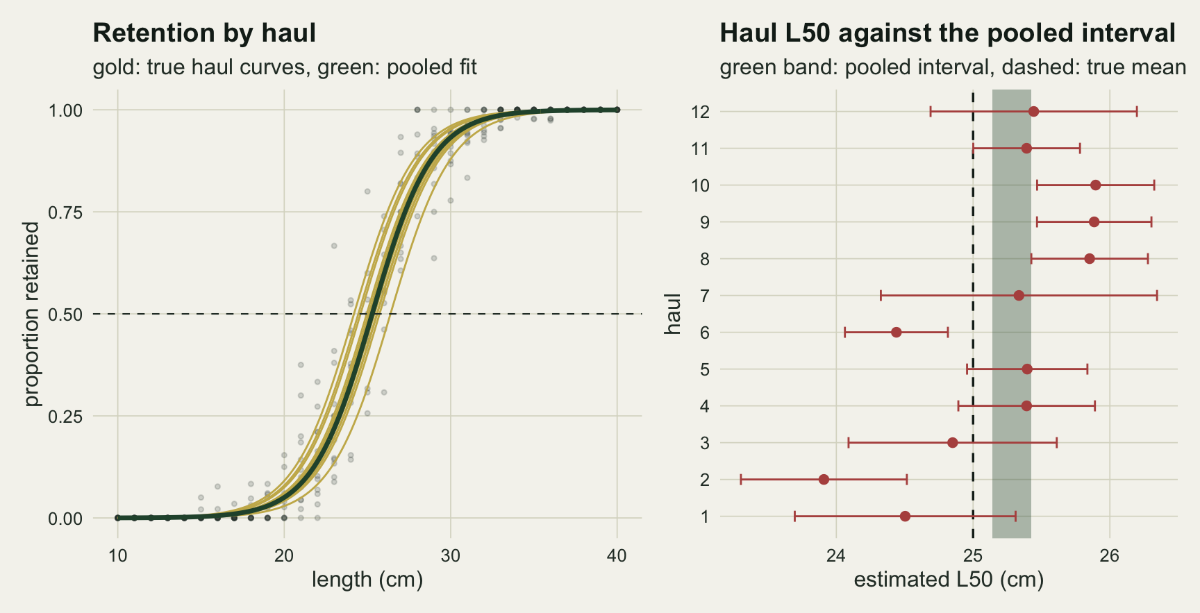
The pooled interval misses, and more hauls do not help
The grid crosses four levels of between-haul standard deviation in L50, from none to 2 cm, with 6, 12 and 24 hauls. Four intervals are built on each dataset. The pooled interval is the binomial fit on all haul by length cells, with a normal quantile. The quasi-binomial interval multiplies the same standard error by the square root of the Pearson dispersion estimated over those cells and uses a t quantile on the residual degrees of freedom, which is what family = quasibinomial does. The haul interval treats the twelve per-haul L50 estimates as a sample and uses their mean with a t interval on hauls minus one degrees of freedom. The random-L50 interval is the REML weighted mean with its standard error, on the same t quantile. Coverage is counted against the true mean L50 of 25 cm, over simulated datasets.
analyse <- function(s) {
  H <- s$H
  pool  <- fit_logit(rep(len_cm, H), as.vector(s$r), as.vector(s$n))
  lpool <- fit_logit(len_cm, rowSums(s$r), rowSums(s$n))
  per   <- vapply(seq_len(H), function(h) fit_logit(len_cm, s$r[, h], s$n[, h]), numeric(7))
  use   <- per["ok", ] == 1 & is.finite(per["se", ]) & per["se", ] > 0
  y_use <- per["l50", use]; v_use <- per["se", use]^2; H_use <- sum(use)
  rm    <- reml_l50(y_use, v_use)
  # stricter rule, added after review: drop separated fits and slopes not clear of zero
  sep   <- use & per["dev", ] < 1e-6
  flat  <- use & !sep & !(is.finite(per["zb", ]) & per["zb", ] > qnorm(0.975))
  use_s <- use & !sep & !flat
  y_s <- per["l50", use_s]; H_s <- sum(use_s)
  rm_s  <- reml_l50(y_s, per["se", use_s]^2)
  tq_s  <- qt(0.975, H_s - 1); hse_s <- sd(y_s) / sqrt(H_s)
  worst <- which(use)[which.max(per["se", use])]   # least informative kept haul
  worst_cls <- if (sep[worst]) 1 else if (flat[worst]) 2 else 0
  phi   <- pool[["x2"]] / pool[["df"]]
  z  <- qnorm(0.975); tq <- qt(0.975, H_use - 1); tc <- qt(0.975, pool[["df"]])
  hbar <- mean(y_use); hse <- sd(y_use) / sqrt(H_use)
  c(est = pool[["l50"]], se = pool[["se"]], phi = phi,
    phi_len  = lpool[["x2"]] / lpool[["df"]],
    cov_pool  = abs(pool[["l50"]] - l50_true) <= z * pool[["se"]],
    cov_quasi = abs(pool[["l50"]] - l50_true) <= tc * pool[["se"]] * sqrt(phi),
    cov_haul  = abs(hbar - l50_true) <= tq * hse,
    cov_reml  = abs(rm[["mu"]] - l50_true) <= tq * rm[["se"]],
    w_pool = 2 * z * pool[["se"]], w_quasi = 2 * tc * pool[["se"]] * sqrt(phi),
    w_haul = 2 * tq * hse, w_reml = 2 * tq * rm[["se"]],
    bad = mean(!use), hbar = hbar, reml = rm[["mu"]],
    cov_haul_s = abs(mean(y_s) - l50_true) <= tq_s * hse_s,
    cov_reml_s = abs(rm_s[["mu"]] - l50_true) <= tq_s * rm_s[["se"]],
    w_haul_s = 2 * tq_s * hse_s, w_reml_s = 2 * tq_s * rm_s[["se"]],
    n_sep = sum(sep), n_flat = sum(flat), n_kept = H_use, bad_s = mean(!use_s),
    worst_cls = worst_cls, worst_n = sum(s$n[, worst]))
}
n_out <- 25
run_cell <- function(H, sd_haul, fish = fish_mean, rho_cell = 0)
  vapply(seq_len(n_rep), function(i) analyse(sim_hauls(H, sd_haul, fish, rho_cell)), numeric(n_out))

sd_grid <- c(0, 0.5, 1, 2); h_grid <- c(6, 12, 24)
set.seed(2291)
grid_runs <- list()
for (H in h_grid) for (sdh in sd_grid) grid_runs[[paste(H, sdh)]] <- run_cell(H, sdh)
meth_lev <- c("pooled binomial", "quasi-binomial", "haul t interval", "random-L50 REML")
cov_tab <- do.call(rbind, lapply(names(grid_runs), function(k) {
  g <- grid_runs[[k]]; hs <- as.numeric(strsplit(k, " ")[[1]])
  data.frame(H = hs[1], sd_haul = hs[2], method = meth_lev,
             coverage = rowMeans(g[c("cov_pool", "cov_quasi", "cov_haul", "cov_reml"), ]),
             width = rowMeans(g[c("w_pool", "w_quasi", "w_haul", "w_reml"), ]),
             phi = mean(g["phi", ]), phi_len = mean(g["phi_len", ]),
             deff = var(g["est", ]) / mean(g["se", ]^2))
}))
cov_tab$method <- factor(cov_tab$method, levels = meth_lev)
cov_tab$mcse <- sqrt(cov_tab$coverage * (1 - cov_tab$coverage) / n_rep)
cv <- function(H, sdh, m) cov_tab$coverage[cov_tab$H == H & cov_tab$sd_haul == sdh & cov_tab$method == meth_lev[m]]
wd <- function(H, sdh, m) cov_tab$width[cov_tab$H == H & cov_tab$sd_haul == sdh & cov_tab$method == meth_lev[m]]
ct <- function(H, sdh, col) cov_tab[cov_tab$H == H & cov_tab$sd_haul == sdh, col][1]
mcse_95 <- sqrt(0.95 * 0.05 / n_rep)
haul_min <- min(cov_tab$coverage[cov_tab$method %in% meth_lev[3:4]])
haul_max <- max(cov_tab$coverage[cov_tab$method %in% meth_lev[3:4]])
With no between-haul variation all four intervals are near nominal. At twelve hauls the pooled binomial interval covers 0.940 of the time, the quasi-binomial 0.923, the haul t interval 0.963 and the REML interval 0.987. The REML interval is on the conservative side here, and reaches 1.000 at six hauls: the t quantile on five degrees of freedom and a between-haul variance estimated above its true value of zero both widen it.
Add a between-haul standard deviation of 1 cm and the pooled interval covers 0.423, 0.407 and 0.410 of the time with 6, 12 and 24 hauls. The quasi-binomial interval covers 0.437, 0.453 and 0.453. At 2 cm the pooled coverage is 0.273, 0.187 and 0.210. The Monte Carlo standard error of any of these rates is at most 0.029. Across all twelve settings the two haul-level intervals cover between 0.933 and 1.000 of the time.
Adding hauls does not rescue the pooled fit, and there is a simple reason. The binomial standard error shrinks with the square root of the number of fish, and the true standard error of the mean L50 shrinks with the square root of the number of hauls. Doubling the hauls shrinks both by the same factor, so their ratio, and with it the coverage, stays where it was.
cov_tab$panel <- factor(sprintf("%d hauls", cov_tab$H), levels = sprintf("%d hauls", h_grid))
ggplot(cov_tab, aes(sd_haul, coverage, colour = method)) +
  geom_hline(yintercept = 0.95, colour = te_body, linetype = "dotted", linewidth = 0.6) +
  geom_errorbar(aes(ymin = coverage - 2 * mcse, ymax = coverage + 2 * mcse),
                width = 0.08, linewidth = 0.4, position = position_dodge(width = 0.15)) +
  geom_line(aes(linetype = method), linewidth = 0.9, position = position_dodge(width = 0.15)) +
  geom_point(size = 1.9, position = position_dodge(width = 0.15)) +
  facet_wrap(~ panel, nrow = 1) +
  scale_colour_manual(values = c(te_rust, te_gold, te_forest, te_ink), name = NULL) +
  scale_linetype_manual(values = c("solid", "solid", "solid", "22"), name = NULL) +
  scale_x_continuous(breaks = sd_grid) +
  scale_y_continuous(limits = c(0, 1)) +
  guides(colour = guide_legend(nrow = 2)) +
  labs(x = "between-haul standard deviation of L50 (cm)", y = "coverage of the true mean L50",
       title = "Only the haul-level intervals hold their coverage",
       subtitle = "dotted line: nominal 95 per cent; REML drawn dashed") +
  theme_datasheet() + theme(legend.position = "bottom", legend.key.width = unit(1.6, "lines"))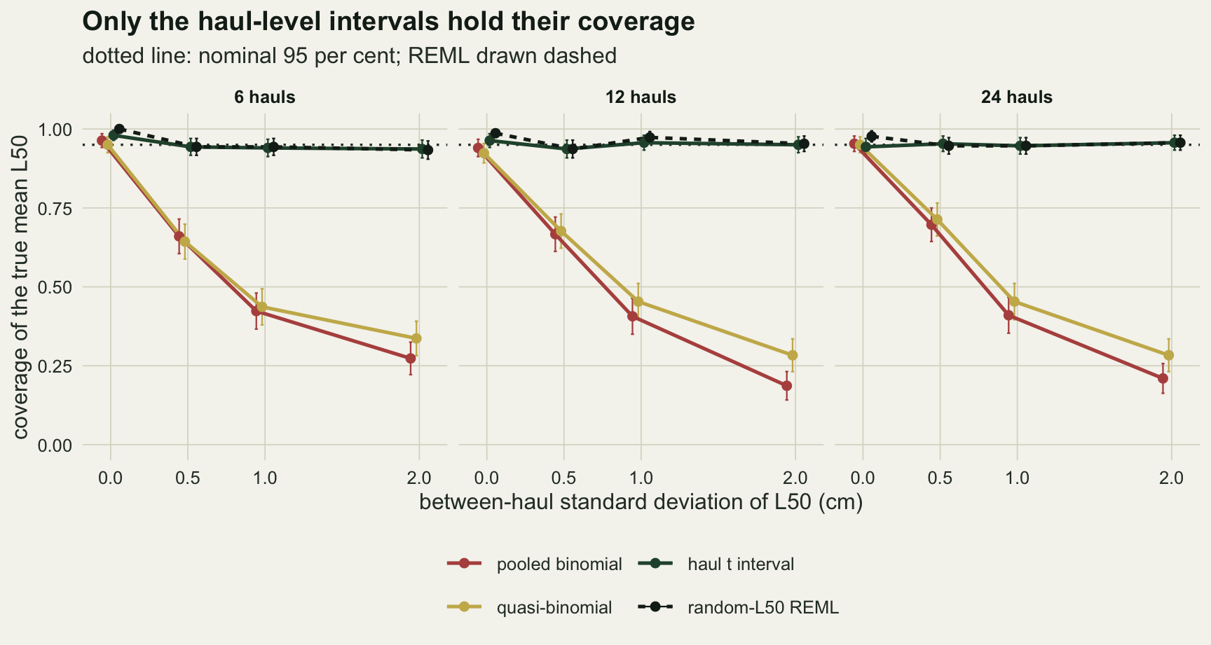
The widths show the size of the gap. At twelve hauls and 1 cm, the pooled interval is on average 0.35 cm wide and the haul t interval 1.33 cm, 3.8 times as wide. The measured design effect for the pooled L50, the variance of the estimate across datasets divided by the mean squared standard error the fit reports, is 12.9. The quasi-binomial correction widens the interval by the square root of the dispersion, here a factor of 1.11, because the mean dispersion it estimates is 1.24.
Why the dispersion statistic does not see a shifted curve
A quasi-binomial correction assumes that the extra variation is independent from cell to cell, so that the variance of every count is inflated by the same factor and the variance of every estimate by that factor too. The contrast case is noise that behaves that way. Here the same twelve hauls have no between-haul shift at all, but every haul by length cell gets its own retention probability drawn from a beta distribution around the true curve, with an intraclass correlation within a cell of 0.01, 0.03 or 0.06. That is the vessel effect of the dose-response check transplanted into a trawl, and the three correlations were picked before the run to span the same range of dispersion as the curve shifts.
rho_grid <- c(0.01, 0.03, 0.06)
set.seed(7730)
cell_runs <- lapply(rho_grid, function(rho) run_cell(12, 0, rho_cell = rho))
cell_tab <- data.frame(source = "independent cell noise", level = rho_grid,
  phi = vapply(cell_runs, function(g) mean(g["phi", ]), 0),
  deff = vapply(cell_runs, function(g) var(g["est", ]) / mean(g["se", ]^2), 0),
  cov_pool = vapply(cell_runs, function(g) mean(g["cov_pool", ]), 0),
  cov_quasi = vapply(cell_runs, function(g) mean(g["cov_quasi", ]), 0))
shift_tab <- data.frame(source = "shift of the haul curve", level = sd_grid[-1],
  phi = vapply(sd_grid[-1], function(s) ct(12, s, "phi"), 0),
  deff = vapply(sd_grid[-1], function(s) ct(12, s, "deff"), 0),
  cov_pool = vapply(sd_grid[-1], function(s) cv(12, s, 1), 0),
  cov_quasi = vapply(sd_grid[-1], function(s) cv(12, s, 2), 0))
disp_tab <- rbind(cell_tab, shift_tab)
phi_len12 <- vapply(sd_grid, function(s) ct(12, s, "phi_len"), 0)
shift_1cm <- abs(plogis(b_true * (len_cm - l50_true - 1)) - plogis(b_true * (len_cm - l50_true)))
shift_max <- max(shift_1cm); n_active <- sum(shift_1cm > 0.05)
cells_12 <- 12 * n_len
With independent cell noise at a correlation of 0.06, the mean dispersion is 2.13 and the design effect for L50 is 2.45. The pooled interval covers 0.793 of the time and the quasi-binomial interval 0.913: the correction recovers most of the lost coverage, though it stops short of 95 per cent, much as it did for the vessels in the dose-response check. With a curve shift of 2 cm the mean dispersion is almost the same, 2.08, but the design effect is 48.9, and the quasi-binomial interval covers only 0.283.
disp_tab$lab <- ifelse(disp_tab$source == "independent cell noise",
                       sprintf("rho %.2f", disp_tab$level), sprintf("SD %.1f cm", disp_tab$level))
ref_line <- data.frame(phi = seq(0.85, 2.3, by = 0.05))
ggplot(disp_tab, aes(phi, deff, colour = source)) +
  geom_line(data = ref_line, aes(phi, phi), inherit.aes = FALSE,
            colour = te_body, linetype = "dashed", linewidth = 0.5) +
  geom_line(linewidth = 0.8) + geom_point(size = 2.6) +
  geom_text(aes(label = lab, vjust = -0.9,
                hjust = ifelse(source == "independent cell noise", 0.5, 1)),
            size = 3.4, show.legend = FALSE) +
  scale_y_log10() +
  scale_colour_manual(values = c(te_forest, te_rust), name = NULL) +
  coord_cartesian(xlim = c(0.85, 2.3), ylim = c(0.8, 80)) +
  labs(x = "Pearson dispersion over haul by length cells",
       y = "design effect for L50 (log scale)",
       title = "The same dispersion, very different design effects",
       subtitle = "dashed line: what the quasi-binomial correction assumes") +
  theme_datasheet() + theme(legend.position = "bottom")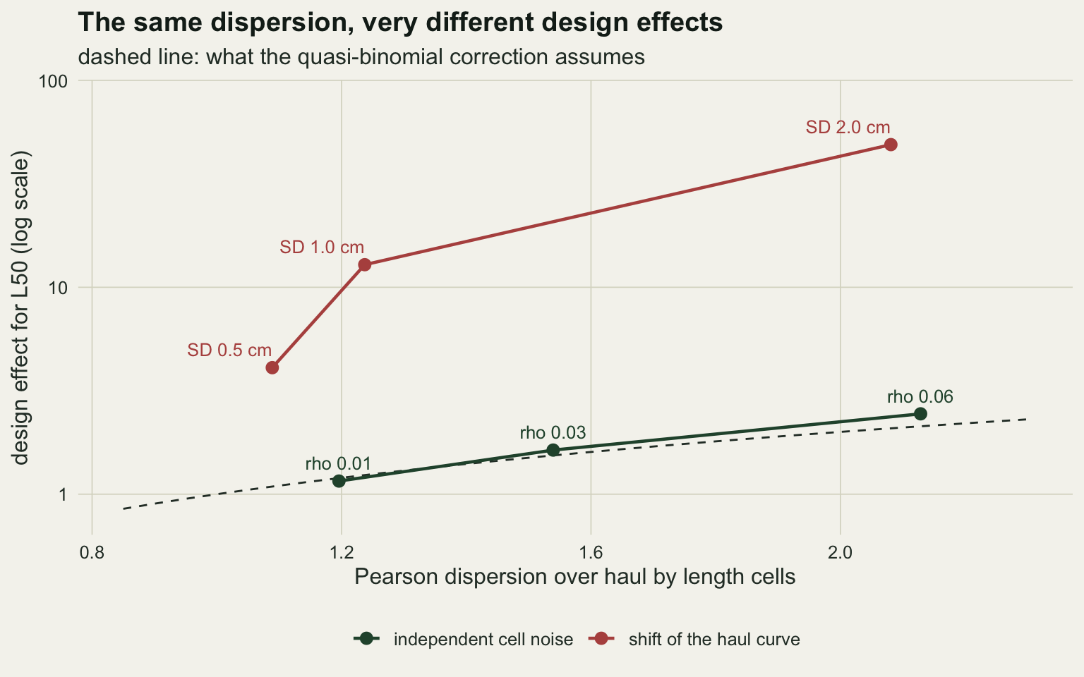
Two things keep the dispersion statistic small when the curve moves. The first is dilution. A shift of 1 cm changes the retention probability by at most 0.134, next to the L50, and by more than 0.05 at only 8 of the 31 length classes. The statistic is an average over all 372 haul by length cells of a twelve-haul trial, and most of those cells hold fish that are always retained or always escape, whatever the haul does.
The second matters more. Within a haul, a shift to the right lowers the retention at every length at once, so the Pearson residuals of that haul all lean the same way. The quasi-binomial correction inflates each cell’s variance but still treats the cells as independent, and it is the correlation between cells of one haul, not the variance of any one of them, that makes the L50 estimate move from trial to trial. A vessel in a toxicity test is one cell, so its effect is all variance and no correlation, and the correction fits it. Pooling over hauls before fitting hides even the variance: a sum of binomial counts with different probabilities is no more variable than one binomial, and the length-pooled dispersion at twelve hauls is 1.01, 1.02, 0.97 and 0.99 for between-haul standard deviations of 0, 0.5, 1 and 2 cm. A dispersion near one in a length-pooled selectivity fit is no evidence that the hauls agree.
Few fish per haul: the weighted model is insurance
With twenty fish per length class the per-haul fits are precise and every haul counts about equally, so a plain t interval on the twelve estimates does as well as the REML model. A lighter tow or a species caught in small numbers is where the weighting ought to start to matter. The last arm keeps twelve hauls and a between-haul standard deviation of 1 cm and lowers the expected catch to 5 and then 2 fish per length class.
fish_grid <- c(2, 5, 20)
set.seed(5518)
sparse_runs <- lapply(fish_grid, function(fm) run_cell(12, 1, fish = fm))
sp_row <- function(g, fm) data.frame(fish = fm, method = meth_lev[3:4],
  coverage = rowMeans(g[c("cov_haul", "cov_reml"), ]),
  width = c(median(g["w_haul", ]), median(g["w_reml", ])),
  bad = mean(g["bad", ]))
sparse_tab <- do.call(rbind, Map(sp_row, sparse_runs, fish_grid))
sparse_tab$method <- factor(sparse_tab$method, levels = meth_lev[3:4])
sparse_tab$mcse <- sqrt(sparse_tab$coverage * (1 - sparse_tab$coverage) / n_rep)
sq <- function(fm, m, col) sparse_tab[sparse_tab$fish == fm & sparse_tab$method == meth_lev[m], col]
sp_pool <- vapply(sparse_runs, function(g) mean(g["cov_pool", ]), 0)
sp_haul_wmax <- vapply(sparse_runs, function(g) max(g["w_haul", ]), 0)
sp_reml_wmax <- vapply(sparse_runs, function(g) max(g["w_reml", ]), 0)
sp_blow <- vapply(sparse_runs, function(g) sum(g["w_haul", ] > 2 * g["w_reml", ]), 0)
# the blow-ups, and what the stricter rule removes
sp_blow_i  <- which(sparse_runs[[1]]["w_haul", ] > 2 * sparse_runs[[1]]["w_reml", ])
sp_blow_sep  <- sum(sparse_runs[[1]]["worst_cls", sp_blow_i] == 1)
sp_blow_flat <- sum(sparse_runs[[1]]["worst_cls", sp_blow_i] == 2)
sp_blow_n    <- sparse_runs[[1]]["worst_n", sp_blow_i]
sp_bad_s     <- vapply(sparse_runs, function(g) mean(g["bad_s", ]), 0)
sp_kept  <- vapply(sparse_runs, function(g) sum(g["n_kept", ]), 0)
sp_sep   <- vapply(sparse_runs, function(g) sum(g["n_sep", ]), 0)
sp_flat  <- vapply(sparse_runs, function(g) sum(g["n_flat", ]), 0)
sp_cov_s <- sapply(sparse_runs, function(g) rowMeans(g[c("cov_haul_s", "cov_reml_s"), ]))
sp_w_s   <- sapply(sparse_runs, function(g) c(median(g["w_haul_s", ]), median(g["w_reml_s", ])))
sp_wmax_s <- sapply(sparse_runs, function(g) c(max(g["w_haul_s", ]), max(g["w_reml_s", ])))
sp_blow_s <- vapply(sparse_runs, function(g) sum(g["w_haul_s", ] > 2 * g["w_reml_s", ]), 0)
sp_cov_nb <- mean(sparse_runs[[1]]["cov_haul", -sp_blow_i])
grid_kept   <- sum(sapply(grid_runs, function(g) sum(g["n_kept", ])))
grid_strict <- sum(sapply(grid_runs, function(g) sum(g["n_sep", ] + g["n_flat", ])))
A haul fit is set aside when it fails to converge, returns a slope that is not positive, or has no finite standard error. The rule was fixed before this arm was run, and it is applied to both haul-level intervals. A stricter rule, added after a review of this post and therefore not fixed in advance, also sets aside separated fits (residual deviance below one in a million, which a fit reaches when retained and escaped fish do not overlap in length or overlap at a single length only) and fits whose slope is not clear of zero, with a Wald statistic below the 97.5 per cent normal quantile; that is also the point at which a Fieller interval for L50 stops being bounded. The main grid uses the original rule; the sparse arm reports both.
p_w <- ggplot(sparse_tab, aes(fish, width, colour = method)) +
  geom_line(aes(linetype = method), linewidth = 0.9) + geom_point(size = 2.2) +
  scale_x_log10(breaks = fish_grid) +
  scale_colour_manual(values = c(te_forest, te_ink), name = NULL) +
  scale_linetype_manual(values = c("solid", "22"), name = NULL) +
  scale_y_continuous(limits = c(0, NA)) +
  labs(x = "expected fish per length class per haul", y = "median interval width (cm)",
       title = "Width", subtitle = "medians over 300 datasets") +
  theme_datasheet() + theme(legend.position = "bottom", legend.key.width = unit(1.6, "lines"))
p_c <- ggplot(sparse_tab, aes(fish, coverage, colour = method)) +
  geom_hline(yintercept = 0.95, colour = te_body, linetype = "dotted", linewidth = 0.6) +
  geom_errorbar(aes(ymin = coverage - 2 * mcse, ymax = coverage + 2 * mcse),
                width = 0.04, linewidth = 0.4, position = position_dodge(width = 0.06)) +
  geom_line(aes(linetype = method), linewidth = 0.9, position = position_dodge(width = 0.06)) +
  geom_point(size = 2.2, position = position_dodge(width = 0.06)) +
  scale_x_log10(breaks = fish_grid) +
  scale_colour_manual(values = c(te_forest, te_ink), name = NULL) +
  scale_linetype_manual(values = c("solid", "22"), name = NULL) +
  scale_y_continuous(limits = c(0.8, 1)) +
  labs(x = "expected fish per length class per haul", y = "coverage",
       title = "Coverage", subtitle = "dotted line: nominal 95 per cent") +
  theme_datasheet() + theme(legend.position = "bottom", legend.key.width = unit(1.6, "lines"))
p_w + p_c + plot_annotation(theme = theme_datasheet())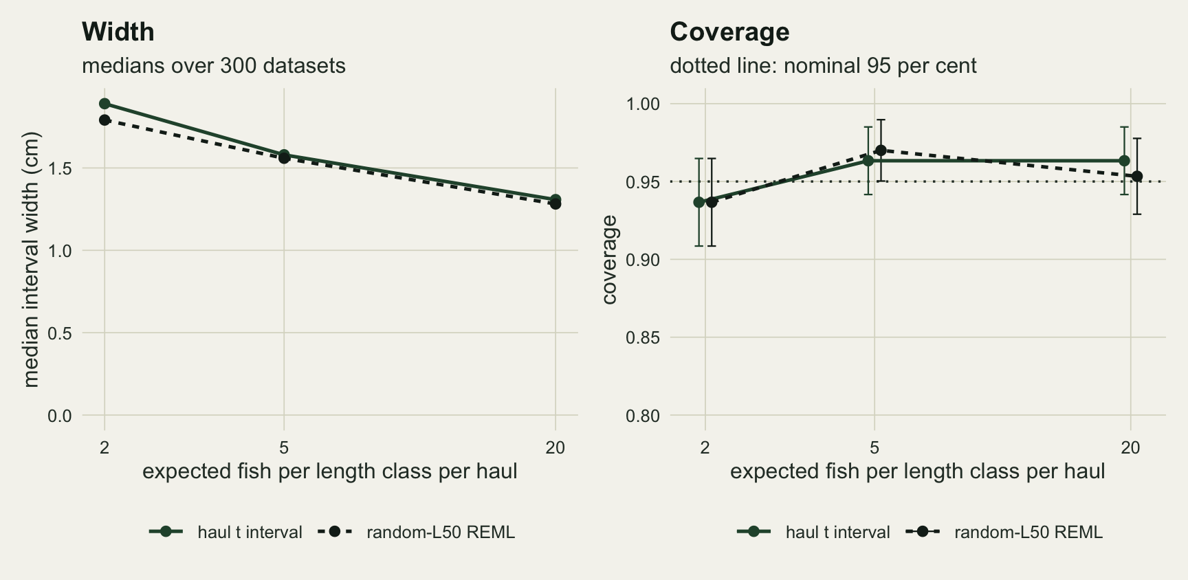
At 2 fish per length class, 10.7 per cent of haul fits are set aside by the rule; at 5 fish it is 1.1 per cent. Coverage of the two haul-level intervals is 0.937 and 0.937 at 2 fish, and 0.963 and 0.953 at 20. The median widths are 1.89 and 1.79 cm at 2 fish, and 1.31 and 1.28 cm at 20. In this design the plain t interval on per-haul estimates is a fair analysis, even with thin catches.
The difference sits in the tail. At 2 fish per length class, 3 of the 300 t intervals under the original rule are more than twice as wide as the REML interval on the same data, and the widest of them has a width of the order of ten to the power 16 cm. In 1 of the 3 datasets the least informative haul the rule kept is a haul of 6 fish whose single retained fish sits exactly at the mean length of the catch. The slope that maximises the likelihood is then zero and the L50 does not exist; glm.fit returns a slope that is positive only by rounding, so the rule lets the haul through, and that haul produces the absurd interval. In the other 2 datasets the least informative kept haul is completely separated: every retained fish is longer than every escaped one, no maximum likelihood estimate exists, and glm.fit still reports convergence, with a standard error that is enormous. The REML model gives such hauls almost no weight, and its widest interval over all 300 datasets is 3.32 cm.
These are not isolated fits. Of the 3216 haul fits the original rule kept at 2 fish, 53 are separated in that sense and another 275 have a slope that is not clear of zero; at 5 fish the counts are 6 and 45 of 3559, and at 20 fish 0 and 0. Over the whole main grid, which has an expected 20 fish per length class, the stricter rule would have removed 7 of 50399 kept fits. The stricter rule has a price: it sets aside 19.8 per cent of haul fits at 2 fish, about one haul in five, and 2.6 per cent at 5. At 2 fish the t interval then covers 0.937 and the REML interval 0.950, with median widths of 1.94 and 1.86 cm, and no t interval is more than twice as wide as the REML one on the same data; the widest t interval is 4.22 cm. Under the original rule, leaving out the 3 blown-up datasets, the t interval covers 0.936. The weighted model is insurance against hauls that the exclusion rule failed to see, not a narrower interval on ordinary data, and a rule that checks for separation and for a flat slope did the same job in this design. The pooled binomial interval, for comparison, covers 0.793 of the time at 2 fish and 0.393 at 20: with thin catches the binomial error is a larger share of the total, so the pooled fit is less wrong, but it is still wrong.
What to report
Report the number of hauls before anything else, and treat it as the sample size for L50. The number of fish measured says how precisely each haul’s curve is known; it says little about how well the mean curve of the gear is known once the hauls differ.
Show the per-haul estimates, as a table or as the right-hand panel of the first figure. A reader can see between-haul variation in that panel at a glance, and no dispersion statistic will show it for them.
Give the mean L50 with an interval built on hauls: a t interval on the per-haul estimates when catches are comparable, or the random-L50 model, which weights hauls by their precision and survives a haul with almost no information. Before a haul enters either interval, check its fit for separation and for a slope that is not clear of zero: glm.fit reports both as converged, and neither has a usable L50. Report the estimated between-haul standard deviation alongside, because it is a property of the gear in use and the next trial will want it.
If catches were pooled over hauls, say so and do not present the pooled binomial interval as the uncertainty of the gear’s L50. If a quasi-binomial or overdispersion check was run and came out near one, do not report that as evidence that the hauls agree. State any rule used to drop hauls and how many it dropped.
Honest limits
Only L50 varies between hauls here, and the selection range is the same in every haul. Real hauls vary in both, and the two need not vary independently. Fryer 1991 carries both curve parameters of each haul together, with a two by two between-haul covariance matrix, and allows haul-level covariates in the mean; the one-parameter REML model in this post is a reduction of that, adequate for an interval on L50 and not for the selection range or for a curve prediction at a given length.
The design is covered-codend throughout, where every fish that enters the codend is accounted for. Many trials instead use alternate hauls or a twin or trouser trawl with a small-meshed control, and there the SELECT method of Millar 1992 fits the selection curve together with a split parameter for the share of fish entering the test gear. Between-haul variation matters there as well, and it enters the split parameter too; nothing in this post measures that case. Millar and Fryer 1999 review both designs and the between-haul question for each.
The catch is spread evenly over lengths 10 to 40 cm. Real length distributions are peaked and differ between hauls, which changes how much information each haul carries about L50 and is likely to make the weighting in the random-L50 model matter more than it does here. Cover effects on escapement, and fish lost or damaged between codend and measuring board, are absent.
The haul exclusion rule used for the main grid is crude. It lets through hauls whose slope is zero to rounding and hauls with complete separation, both of which glm.fit reports as converged, and it could not see the fits that produced the wide t intervals in the sparse arm. The stricter rule catches both kinds here, but it was written after those failures were found. Its deviance test finds separation, including the case where retained and escaped fish overlap at a single length, because the fit is then saturated; its slope check leans on a Wald statistic, which is known to shrink towards zero near separation and is a crude judge of a slope estimated from a handful of fish, where a likelihood ratio test would be the better check and is not explored here. Any rule that looks at the fitted curve is data dependent. The intervals use a delta-method standard error for each haul and a t quantile on hauls minus one degrees of freedom for the mean; other choices, such as profile intervals per haul or a small-sample correction for the REML standard error, are not explored.
The target throughout is the mean L50 over hauls. That is only the L50 of the gear in commercial use if the trial’s hauls are a fair sample of the conditions the gear fishes in, which a research cruise of twelve hauls in one season rarely is. Coverage of 95 per cent here means 95 per cent over hauls like these.
References
Fryer RJ 1991 ICES Journal of Marine Science 48(3):281-290 (10.1093/icesjms/48.3.281)
Millar RB 1992 Journal of the American Statistical Association 87(420):962-968 (10.1080/01621459.1992.10476250)
Millar RB, Fryer RJ 1999 Reviews in Fish Biology and Fisheries 9(1):89-116 (10.1023/A:1008838220001)