library(ggplot2)
library(patchwork)

te_paper  <- "#f5f4ee"
te_ink    <- "#16241d"
te_body   <- "#2c3a31"
te_forest <- "#275139"
te_rust   <- "#b5534e"
te_gold   <- "#c9b458"
te_line   <- "#dad9ca"

theme_datasheet <- function() {
  theme_minimal(base_size = 12) +
    theme(plot.background  = element_rect(fill = te_paper, colour = NA),
          panel.background = element_rect(fill = te_paper, colour = NA),
          panel.grid.major = element_line(colour = te_line, linewidth = 0.3),
          panel.grid.minor = element_blank(),
          text             = element_text(colour = te_body),
          plot.title       = element_text(colour = te_ink, face = "bold"),
          plot.subtitle    = element_text(colour = te_body),
          axis.text        = element_text(colour = te_body))
}Change-in-ratio population estimates in R
R
abundance
harvest
population ecology
ecology tutorial
Population size from a sex ratio measured before and after a known harvest. Why the estimate divides by the ratio change, and when it stops meaning anything.
A deer herd is counted twice in a season, once in late summer and once after a bucks-only hunting season. Neither count finds every animal, and nobody has marked any of them. What the observers do get right is the class of each deer they see: antlered male or not. The hunting season, meanwhile, produces a number that is known almost exactly, because every harvested buck is checked at a registration station. The proportion of males in the classified sample falls between the two counts, and the size of that fall, set against the known number removed, says how large the herd was. If four hundred bucks come out of a small herd, the sex ratio collapses; out of a large herd, it barely moves.
This is the change-in-ratio method, and the version used here is the two class estimator in the form, and with the variance, given by Paulik and Robson (1969) and later set out in Seber (1982). It needs no marks, no detection model and no repeated visits to the same animals. What it needs is a ratio that actually changes, and the price of a small change is the subject of this post.
The site already has two estimators with the same weak point. The post on removal and depletion sampling computes the classic two pass estimate, the first catch squared over the difference between the first and second catches, and gets a population far above the five pass estimate because the drop between the first two catches happened to be gentle. It explains the failure in one sentence and moves on to more passes. The post on closed-population capture-recapture notes that the Lincoln-Petersen ratio is biased upward when the number of recaptures is small, because a small denominator swings the estimate, and uses Chapman’s correction. Both are a count divided by a quantity that can be close to zero. The change-in-ratio estimator is the cleanest case of that structure, because the denominator is literally a difference of two sample proportions, and this post measures what the small denominator does: to the spread, to the point estimate, to the mean and to the interval.
The estimator from a harvest and two classified counts
Write the herd before the season as having a total of N1 animals, of which a proportion p1 are males. The season removes Rx males and Ry females, R in total. After the season the herd has N1 minus R animals and a proportion p2 of males. Counting males before and after gives the identity p2 (N1 - R) = p1 N1 - Rx, and solving for N1 gives
\[\hat N_1 = \frac{R_x - R\,\hat p_2}{\hat p_1 - \hat p_2},\]
with the two proportions replaced by their estimates from the classified samples. That is the two class change-in-ratio estimator as Paulik and Robson write it, and it is linear in the known removals and hyperbolic in the proportions. For a bucks-only season Ry is zero, R equals Rx, and the numerator becomes Rx times one minus the post-season proportion of males.
The design below was fixed before any simulation ran. The herd holds 2000 deer, half of them males. Each survey classifies 800 animals, drawn as a binomial sample, which is the sampling model behind the usual variance formula and a fair description of a roadside count where the same deer can be seen more than once. Two seasons are compared: a heavy harvest of 400 bucks and a light harvest of 150.
herd_n   <- 2000           # N1, deer before the season
males_n  <- 1000           # males before the season
p1_true  <- males_n / herd_n
n_class  <- 800            # animals classified in each survey
rx_heavy <- 400            # bucks removed, heavy season
rx_light <- 150            # bucks removed, light season

p2_of <- function(rx, ry = 0) (males_n - rx) / (herd_n - rx - ry)

cir_est <- function(p1_hat, p2_hat, rx, ry = 0) {
  r_tot <- rx + ry
  (rx - r_tot * p2_hat) / (p1_hat - p2_hat)
}

p2_heavy <- p2_of(rx_heavy)
p2_light <- p2_of(rx_light)
d_heavy  <- p1_true - p2_heavy
d_light  <- p1_true - p2_light
The heavy season takes the proportion of males from 0.500 to 0.375, a change of 0.125. The light season takes it to 0.459, a change of 0.041.
set.seed(2208)
y1_obs <- rbinom(1, n_class, p1_true)
y2_obs <- rbinom(1, n_class, p2_heavy)
p1_obs <- y1_obs / n_class
p2_obs <- y2_obs / n_class
n_hat_obs <- cir_est(p1_obs, p2_obs, rx_heavy)
c(males_before = y1_obs, males_after = y2_obs, n_hat = round(n_hat_obs))
males_before males_after n_hat
414 312 1914 In one simulated heavy season the first survey classifies 414 of the 800 deer as males and the second 312. The estimate is 1914 deer against a true 2000.
The variance divides by the square of the change
The delta method gives the approximate variance. The partial derivative of the estimator with respect to the first proportion is minus N1 over the change in proportion, and with respect to the second it is N1 minus R over the same change. With independent binomial surveys of sizes n1 and n2,
\[\operatorname{Var}(\hat N_1) \approx \frac{N_1^2\,p_1(1-p_1)/n_1 + (N_1 - R)^2\,p_2(1-p_2)/n_2}{(p_1 - p_2)^2}.\]
The numerator is the ordinary sampling noise of the two proportions scaled up to herd size. The denominator is the square of the ratio change, so the standard error is inversely proportional to the change itself. A derivation written down by hand deserves a numerical check before anything is built on it.
delta_var <- function(n1_pop, p1, p2, r_tot, n1, n2) {
  (n1_pop^2 * p1 * (1 - p1) / n1 +
     (n1_pop - r_tot)^2 * p2 * (1 - p2) / n2) / (p1 - p2)^2
}
step_h <- 1e-6
grad_num <- c((cir_est(p1_true + step_h, p2_heavy, rx_heavy) -
                 cir_est(p1_true - step_h, p2_heavy, rx_heavy)) / (2 * step_h),
              (cir_est(p1_true, p2_heavy + step_h, rx_heavy) -
                 cir_est(p1_true, p2_heavy - step_h, rx_heavy)) / (2 * step_h))
grad_formula <- c(-herd_n / d_heavy, (herd_n - rx_heavy) / d_heavy)
grad_gap <- max(abs(grad_num - grad_formula) / abs(grad_formula))

cv_heavy <- sqrt(delta_var(herd_n, p1_true, p2_heavy, rx_heavy, n_class, n_class)) / herd_n
cv_light <- sqrt(delta_var(herd_n, p1_true, p2_light, rx_light, n_class, n_class)) / herd_n
se_obs <- sqrt(delta_var(n_hat_obs, p1_obs, p2_obs, rx_heavy, n_class, n_class))
z_light <- d_light / sqrt(p1_true * (1 - p1_true) / n_class + p2_light * (1 - p2_light) / n_class)
The two analytical derivatives agree with central finite differences to a relative error of 6.2e-11. At the true parameter values the delta method coefficient of variation is 17.9 per cent for the heavy season and 59.3 per cent for the light one. The worked survey above has a plug-in standard error of 335 deer.
Those two coefficients of variation are the whole case against a light season if the delta method is right, and the rest of the post is about the ways it is not. A coefficient of variation of that size is not a wide interval around a usable number. In the light season the true ratio change is only 1.6 standard errors away from zero, and a difference of two sample proportions that close to zero will sometimes be zero or negative.
What the sampling distribution looks like
n_rep <- 10000
set.seed(5513)
sim_season <- function(rx, p2) {
  y1 <- rbinom(n_rep, n_class, p1_true)
  y2 <- rbinom(n_rep, n_class, p2)
  data.frame(y1 = y1, y2 = y2,
             n_hat = cir_est(y1 / n_class, y2 / n_class, rx))
}
sim_heavy <- sim_season(rx_heavy, p2_heavy)
sim_light <- sim_season(rx_light, p2_light)

summ_season <- function(sim, rx) {
  ok <- is.finite(sim$n_hat)
  est <- sim$n_hat[ok]
  c(undefined  = mean(!ok),
    impossible = mean(!ok | sim$n_hat < rx),
    negative   = mean(sim$n_hat[ok] < 0),
    median     = median(est),
    mean       = mean(est),
    sd_cv      = sd(est) / herd_n,
    iqr_cv     = IQR(est) / (2 * qnorm(0.75)) / herd_n,
    q025       = unname(quantile(est, 0.025)),
    q975       = unname(quantile(est, 0.975)))
}
s_heavy <- summ_season(sim_heavy, rx_heavy)
s_light <- summ_season(sim_light, rx_light)
med_level <- (0.5 - s_light["negative"]) / (1 - s_light["negative"])
round(rbind(heavy = s_heavy, light = s_light), 3)
undefined impossible negative median mean sd_cv iqr_cv q025
heavy 0.000 0.000 0.000 2000.000 2081.382 0.235 0.181 1489.031
light 0.005 0.052 0.047 1842.857 2489.422 4.196 0.572 -7975.781
q975
heavy 3141.007
light 15675.000Each season was simulated 10000 times. The spread is summarised two ways: the standard deviation, and the interquartile range divided by 1.349, which equals the standard deviation for a normal distribution but ignores the tails.
In the heavy season the distribution behaves. The median estimate is 2000, the mean 2081, and the interquartile coefficient of variation 18.1 per cent against the delta method’s 17.9. The standard deviation gives 23.5 per cent, noticeably larger, because a ratio is skewed to the right even when its denominator stays well clear of zero, and the right tail inflates a standard deviation more than it moves the quartiles. The central 95 per cent of estimates runs from 1489 to 3141.
The light season is a different kind of object. The interquartile coefficient of variation is 57.2 per cent, which is still in line with the delta method’s 59.3, so the delta method describes the middle of the distribution accurately. The standard deviation is 420 per cent of the herd. The central 95 per cent of estimates runs from -7976 to 15675: the lower end is a negative number of deer. Of all simulated light seasons, 5.2 per cent give an estimate that is undefined or smaller than the number of bucks already shot, and 0.54 per cent have exactly equal proportions of males in the two surveys, so the estimator divides by zero.
show_lo <- -4000; show_hi <- 10000
hist_df <- rbind(
  data.frame(season = "heavy harvest, 400 bucks", n_hat = sim_heavy$n_hat),
  data.frame(season = "light harvest, 150 bucks", n_hat = sim_light$n_hat))
hist_df <- hist_df[is.finite(hist_df$n_hat), ]
out_share <- tapply(hist_df$n_hat < show_lo | hist_df$n_hat > show_hi,
                    hist_df$season, mean)
lab_df <- data.frame(season = names(out_share),
                     lab = sprintf("%.2f per cent outside the panel", 100 * out_share))
hist_df <- hist_df[hist_df$n_hat >= show_lo & hist_df$n_hat <= show_hi, ]

ggplot(hist_df, aes(n_hat)) +
  annotate("rect", xmin = show_lo, xmax = 0, ymin = -Inf, ymax = Inf,
           fill = te_rust, alpha = 0.08) +
  geom_histogram(binwidth = 200, boundary = 0, fill = te_forest, colour = NA) +
  geom_vline(xintercept = herd_n, linetype = "dashed", colour = te_rust,
             linewidth = 0.7) +
  geom_text(data = lab_df, aes(x = show_hi, y = Inf, label = lab),
            hjust = 1, vjust = 1.6, colour = te_body, size = 3.6) +
  facet_wrap(~ season, ncol = 1, scales = "free_y") +
  labs(x = "estimated herd size", y = "simulated seasons",
       title = "A small ratio change changes the shape, not just the width",
       subtitle = "dashed: the true herd of 2000; shaded: negative estimates") +
  theme_datasheet() +
  theme(strip.text = element_text(colour = te_ink, face = "bold", hjust = 0))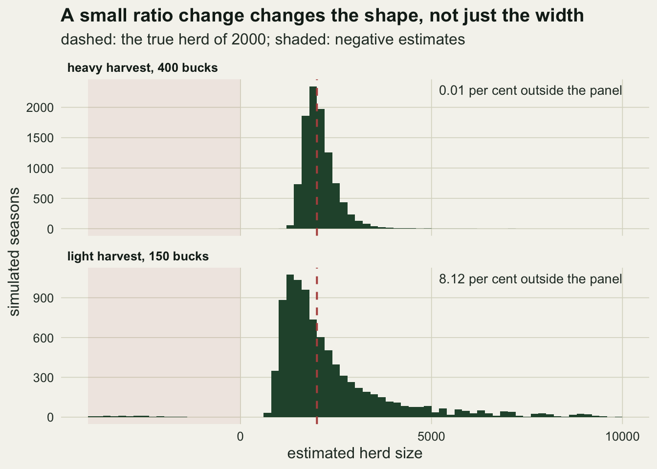
The median is not safe either, and the mean does not exist
A common piece of advice for a ratio estimator with a heavy tail is to report the median, on the grounds that it is close to unbiased when the mean is not. In the heavy season that holds: the median is 2000 for a true herd of 2000. In the light season the median is 1843, 7.9 per cent below the truth. The reason is the sign change. The estimate is a decreasing function of the observed ratio change on each side of zero, but when the observed change crosses zero the estimate jumps from a very large positive number to a very large negative one. The negative estimates, 4.7 per cent of the defined ones, all land in the lower tail, although they come from the seasons whose estimate should have been largest. The overall median is therefore the 47.6 percentile of the positive estimates rather than their fiftieth.
The claim that the mean does not exist can be made exactly. With binomial surveys, the two sample proportions are equal with a probability that is small but not zero, and on that event the estimator is undefined. An estimator that is undefined with positive probability has no expectation at all. That probability is a single sum over the possible counts of males.
p_tie <- function(p2) sum(dbinom(0:n_class, n_class, p1_true) *
                            dbinom(0:n_class, n_class, p2))
tie_heavy <- p_tie(p2_heavy)
tie_light <- p_tie(p2_light)
tie_sim_se <- sqrt(tie_light * (1 - tie_light) / n_rep)

# exact conditional mean (ties excluded) by enumerating every pair of counts
counts   <- 0:n_class
pair_w   <- outer(dbinom(counts, n_class, p1_true), dbinom(counts, n_class, p2_light))
pair_est <- outer(counts / n_class, counts / n_class,
                  function(a, b) cir_est(a, b, rx_light))
pair_gap <- abs(outer(counts, counts, "-"))
pair_ok  <- is.finite(pair_est)
w_ok     <- sum(pair_w[pair_ok])
cond_mean_light <- sum(pair_w[pair_ok] * pair_est[pair_ok]) / w_ok
cond_sd_light   <- sqrt(sum(pair_w[pair_ok] * (pair_est[pair_ok] - cond_mean_light)^2) / w_ok)
excess_light    <- cond_mean_light - herd_n
excess_from <- function(max_gap) {
  sel <- pair_ok & pair_gap <= max_gap
  sum(pair_w[sel] * (pair_est[sel] - herd_n)) / w_ok
}
excess_gap2  <- excess_from(2)
excess_gap20 <- excess_from(20)
The exact probability of a tie is 5.53e-08 in the heavy season and 0.0053 in the light season. The simulated share of ties in the light season, 0.0054, sits within 0.1 Monte Carlo standard errors of the exact value.
That argument is strictly correct but it is also a technicality, and it helps to be clear about what it does not say. Once the ties are excluded, the counts of males can only take finitely many values, so the conditional mean exists and is a finite number. Enumerating every pair of counts gives it exactly: 2349 deer in the light season, 349 above the true herd. The seasons whose two counts of males differ by at most two animals, where the estimates are largest in absolute value, contribute only 19 per cent of that excess, because a positive and a negative difference of the same size are almost equally likely and their huge estimates of opposite sign nearly cancel. The excess is built over the seasons whose counts differ by up to twenty animals, which together add 545 deer, more than the whole excess; the remaining seasons pull the mean back down by 196. The stronger statement belongs to the large sample approximation, in which the difference of proportions is normal. A ratio whose denominator has a positive density at zero has no finite mean, for the same reason that the Cauchy distribution has none. So the honest summary is that the mean is undefined under the discrete model, exists but is a poor summary after conditioning, and does not exist under the normal approximation that the delta method itself relies on. What the simulation shows is what each of those means for a running average.
light_ok  <- sim_light$n_hat[is.finite(sim_light$n_hat)]
heavy_ok  <- sim_heavy$n_hat[is.finite(sim_heavy$n_hat)]
run_df <- rbind(
  data.frame(rep = seq_along(light_ok), value = cumsum(light_ok) / seq_along(light_ok),
             summary = "running mean, light season"),
  data.frame(rep = seq_along(heavy_ok), value = cumsum(heavy_ok) / seq_along(heavy_ok),
             summary = "running mean, heavy season"))
run_light <- cumsum(light_ok) / seq_along(light_ok)
run_heavy <- cumsum(heavy_ok) / seq_along(heavy_ok)
max_abs_light <- max(abs(light_ok))
half_idx <- function(v) v[seq(floor(length(v) / 2), length(v))]
light_span <- diff(range(half_idx(run_light)))
heavy_span <- diff(range(half_idx(run_heavy)))
max_possible <- rx_light * n_class
mc_se_light  <- cond_sd_light / sqrt(length(light_ok))
mc_z_light   <- (s_light["mean"] - cond_mean_light) / mc_se_light
In the light season the largest single estimate in absolute value is 65700 deer. No defined estimate can exceed 120000 in absolute value, the harvest times the survey size, because the smallest non-zero difference of two proportions out of 800 is one over 800; that bound is why a conditional mean exists at all, not a reason for a simulated average to settle. The exact conditional mean is 2349, 17.4 per cent above the true herd, and the exact conditional standard deviation is 405 per cent of the herd, so a mean of 9946 defined estimates has a Monte Carlo standard error of 81 deer. The running mean ends at 2489, 1.7 Monte Carlo standard errors above the exact value, and over the second half of the run it still moves across 120 deer against 14 in the heavy season. So the conditional mean is a finite number held up by seasons with small ratio changes: a heavy tail, not a divergence, and not a quantity to report.
ggplot(run_df, aes(rep, value, colour = summary)) +
  geom_hline(yintercept = herd_n, linetype = "dashed", colour = te_body,
             linewidth = 0.6) +
  geom_line(linewidth = 0.7) +
  scale_colour_manual(values = c(te_forest, te_rust), name = NULL) +
  scale_x_log10() +
  labs(x = "simulated seasons (log scale)", y = "running mean of the estimate",
       title = "The light season's running mean is moved by single seasons",
       subtitle = "dashed: the true herd of 2000") +
  theme_datasheet() +
  theme(legend.position = "bottom")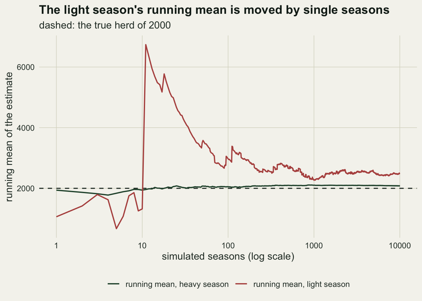
How much change is enough
The two seasons are two points on a curve. Running the same comparison over a range of harvests shows where the estimator stops behaving.
rx_grid <- seq(50, 600, by = 50)
set.seed(7730)
sweep_tab <- do.call(rbind, lapply(rx_grid, function(rx) {
  p2 <- p2_of(rx)
  y1 <- rbinom(n_rep, n_class, p1_true)
  y2 <- rbinom(n_rep, n_class, p2)
  est <- cir_est(y1 / n_class, y2 / n_class, rx)
  ok <- is.finite(est)
  data.frame(rx = rx, change = p1_true - p2,
             delta_cv = sqrt(delta_var(herd_n, p1_true, p2, rx, n_class, n_class)) / herd_n,
             iqr_cv = IQR(est[ok]) / (2 * qnorm(0.75)) / herd_n,
             med_bias = median(est[ok]) / herd_n - 1,
             impossible = mean(!ok | est < rx))
}))
sd_change <- function(rx) sqrt(p1_true * (1 - p1_true) / n_class +
                                 p2_of(rx) * (1 - p2_of(rx)) / n_class)
sweep_tab$z_change <- sweep_tab$change / sd_change(sweep_tab$rx)
round(sweep_tab, 3)
rx change delta_cv iqr_cv med_bias impossible z_change
1 50 0.013 1.925 0.894 -0.622 0.313 0.513
2 100 0.026 0.926 0.623 -0.248 0.152 1.053
3 150 0.041 0.593 0.559 -0.081 0.058 1.624
4 200 0.056 0.427 0.450 -0.013 0.013 2.229
5 250 0.071 0.327 0.344 -0.002 0.002 2.872
6 300 0.088 0.261 0.275 -0.001 0.000 3.557
7 350 0.106 0.214 0.219 -0.003 0.000 4.291
8 400 0.125 0.179 0.177 -0.002 0.000 5.080
9 450 0.145 0.152 0.149 -0.005 0.000 5.933
10 500 0.167 0.130 0.133 0.002 0.000 6.860
11 550 0.190 0.112 0.112 0.000 0.000 7.875
12 600 0.214 0.098 0.098 -0.001 0.000 8.994imp_se_max <- sqrt(0.25 / n_rep)
cv_ratio <- sweep_tab$iqr_cv / sweep_tab$delta_cv
cv_ratio_range <- range(cv_ratio)
agree_tol <- 0.10
rx_agree <- min(sweep_tab$rx[vapply(seq_along(cv_ratio),
function(i) all(abs(cv_ratio[i:length(cv_ratio)] - 1) <= agree_tol), TRUE)])
first_ok <- min(sweep_tab$rx[sweep_tab$impossible < 0.001])
z_first_ok <- sweep_tab$z_change[sweep_tab$rx == first_ok]
imp_50 <- sweep_tab$impossible[sweep_tab$rx == 50]
cv_50 <- sweep_tab$delta_cv[sweep_tab$rx == 50]Across harvests from 50 to 600 bucks, the ratio of the interquartile coefficient of variation to the delta method one runs from 0.46 to 1.05. From 150 bucks upward it stays within 10 per cent of one, so over that range the delta method describes the middle of the distribution well. Below it the delta method overstates the central spread, by a factor of 2.2 at 50 bucks, while the real damage sits in a tail the formula cannot describe at all.
A clearer guide is the expected ratio change in units of its standard error. At a harvest of 50 bucks the delta method coefficient of variation is 193 per cent and 31.3 per cent of seasons give an undefined or impossible estimate. The share of impossible estimates first drops below one in a thousand at 300 bucks, where the true ratio change is 3.6 standard errors from zero. Every share on this grid has a Monte Carlo standard error of at most 0.005.
cv_long <- rbind(
  data.frame(change = sweep_tab$change, cv = sweep_tab$delta_cv, kind = "delta method"),
  data.frame(change = sweep_tab$change, cv = sweep_tab$iqr_cv, kind = "simulated (quartiles)"))

p_cv <- ggplot(cv_long, aes(change, 100 * cv, colour = kind, shape = kind)) +
  geom_line(data = cv_long[cv_long$kind == "delta method", ], linewidth = 0.9) +
  geom_point(data = cv_long[cv_long$kind != "delta method", ], size = 2.4) +
  geom_vline(xintercept = c(d_light, d_heavy), linetype = "dashed",
             colour = te_body, linewidth = 0.5) +
  scale_colour_manual(values = c(te_forest, te_rust), name = NULL) +
  scale_shape_manual(values = c(NA, 16), name = NULL) +
  guides(colour = guide_legend(override.aes = list(linetype = c(1, 0)))) +
  labs(x = "true change in the proportion of males",
       y = "coefficient of variation (per cent)",
       title = "Spread") +
  theme_datasheet() +
  theme(legend.position = "bottom")

p_imp <- ggplot(sweep_tab, aes(change, 100 * impossible)) +
  geom_line(colour = te_rust, linewidth = 0.9) +
  geom_point(colour = te_rust, size = 2.4) +
  geom_vline(xintercept = c(d_light, d_heavy), linetype = "dashed",
             colour = te_body, linewidth = 0.5) +
  labs(x = "true change in the proportion of males",
       y = "undefined or impossible (per cent)",
       title = "Failures") +
  theme_datasheet()

p_cv + p_imp +
  plot_annotation(title = "Precision and failure both hinge on the ratio change",
                  subtitle = "dashed: the light and the heavy season",
                  theme = theme_datasheet())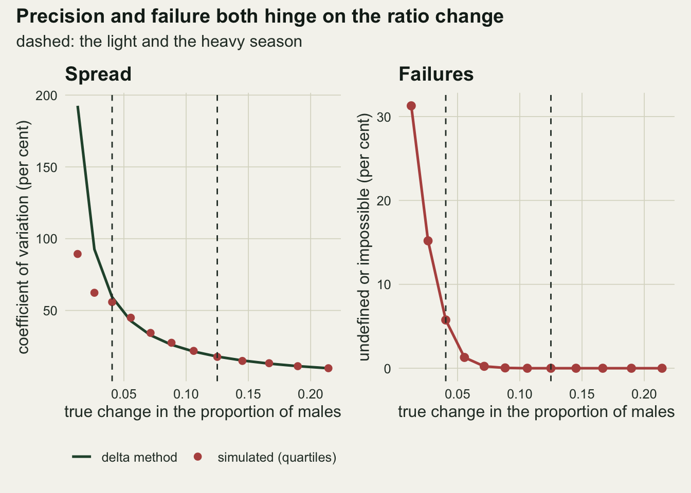
The interval says so, if it is the right interval
A Wald interval built from the delta method standard error is symmetric by construction, so in a light season it runs happily into negative herd sizes. The profile likelihood interval behaves differently. For a bucks-only season the likelihood is the product of the two binomial surveys, with the post-season proportion of males written as the pre-season males minus the harvest, over the herd minus the harvest. For each candidate herd size the pre-season proportion is maximised out, and the interval is the set of herd sizes whose likelihood ratio statistic stays below the chi squared cut.
binom_ll <- function(y, n, p) {
  ifelse(y == 0, 0, y * log(p)) + ifelse(y == n, 0, (n - y) * log1p(-p))
}
prof_ll <- function(n_pop, y1, y2, rx) {
  obj <- function(a) {
    q <- (a * n_pop - rx) / (n_pop - rx)
    binom_ll(y1, n_class, a) + binom_ll(y2, n_class, q)
  }
  optimize(obj, c(rx / n_pop + 1e-9, 1 - 1e-9), maximum = TRUE)$objective
}
# the supremum: the free binomial fit if the proportion fell, else the pooled fit
sup_ll <- function(y1, y2) {
  if (y1 > y2) return(binom_ll(y1, n_class, y1 / n_class) + binom_ll(y2, n_class, y2 / n_class))
  pooled <- (y1 + y2) / (2 * n_class)
  binom_ll(y1, n_class, pooled) + binom_ll(y2, n_class, pooled)
}
lr_stat <- function(n_pop, y1, y2, rx) 2 * (sup_ll(y1, y2) - prof_ll(n_pop, y1, y2, rx))
lr_at_infinity <- function(y1, y2) {
  pooled <- (y1 + y2) / (2 * n_class)
  2 * (sup_ll(y1, y2) - binom_ll(y1, n_class, pooled) - binom_ll(y2, n_class, pooled))
}
cut95 <- qchisq(0.95, 1)
As the candidate herd size grows without limit, the post-season proportion is forced towards the pre-season one, so the profile likelihood approaches the fit in which the ratio did not change at all. That gives an exact rule: the profile interval has a finite upper limit only if the likelihood ratio test that the ratio did not change rejects at the same level. When the survey cannot tell that the ratio moved, the interval says the herd could be any size above its lower limit, which is the correct answer. It is the same behaviour Fieller (1954) described for a ratio of two estimates whose denominator is not distinguishable from zero, and that the post on confidence intervals for effective doses meets when a dose-response slope is too weak.
n_cov <- 5000
cover_season <- function(rx, p2, seed) {
  set.seed(seed)
  y1 <- rbinom(n_cov, n_class, p1_true)
  y2 <- rbinom(n_cov, n_class, p2)
  p1h <- y1 / n_class; p2h <- y2 / n_class
  est <- cir_est(p1h, p2h, rx)
  se  <- sqrt(delta_var(est, p1h, p2h, rx, n_class, n_class))
  wald_in <- is.finite(est) & abs(est - herd_n) <= qnorm(0.975) * se
  lr_true <- mapply(function(a, b) lr_stat(herd_n, a, b, rx), y1, y2)
  open_top <- mapply(lr_at_infinity, y1, y2) < cut95
  c(wald = mean(wald_in), wald_neg = mean(is.finite(est) & est - qnorm(0.975) * se < 0),
    profile = mean(lr_true <= cut95), open_top = mean(open_top))
}
cov_heavy <- cover_season(rx_heavy, p2_heavy, 4101)
cov_light <- cover_season(rx_light, p2_light, 4102)
cov_se <- sqrt(0.05 * 0.95 / n_cov)
round(rbind(heavy = cov_heavy, light = cov_light), 4)
wald wald_neg profile open_top
heavy 0.933 0.0008 0.9490 0.0008
light 0.872 0.5980 0.9558 0.6428Each coverage is the share of 5000 simulated seasons whose interval contains the true herd, with a Monte Carlo standard error of about 0.003 at 95 per cent. In the heavy season the Wald interval covers in 93.3 per cent of seasons and the profile interval in 94.9 per cent, and 0.1 per cent of profile intervals have no upper limit.
In the light season the Wald interval covers in 87.2 per cent of seasons, and 59.8 per cent of Wald intervals reach below zero deer. The profile interval covers in 95.6 per cent, and it does so honestly: 64.3 per cent of the light season profile intervals have no upper limit. That share is the probability that the surveys fail to detect the change in sex ratio with a likelihood ratio test at the 5 per cent level, and it is the most useful single number in this post for deciding whether a change-in-ratio survey is worth running.
set.seed(9120)
y1_l <- rbinom(1, n_class, p1_true)
y2_l <- rbinom(1, n_class, p2_light)
n_grid <- round(exp(seq(log(rx_heavy + 50), log(60000), length.out = 160)))
prof_df <- rbind(
  data.frame(n_pop = n_grid, season = "heavy harvest (the worked survey)",
             lr = vapply(n_grid, lr_stat, 0, y1 = y1_obs, y2 = y2_obs, rx = rx_heavy)),
  data.frame(n_pop = n_grid, season = "light harvest",
             lr = vapply(n_grid, lr_stat, 0, y1 = y1_l, y2 = y2_l, rx = rx_light)))
inf_df <- data.frame(season = c("heavy harvest (the worked survey)", "light harvest"),
                     lr_inf = c(lr_at_infinity(y1_obs, y2_obs), lr_at_infinity(y1_l, y2_l)))
n_hat_l <- cir_est(y1_l / n_class, y2_l / n_class, rx_light)
lo_heavy <- uniroot(function(n) lr_stat(n, y1_obs, y2_obs, rx_heavy) - cut95,
                    c(rx_heavy + 1, n_hat_obs))$root
hi_heavy <- uniroot(function(n) lr_stat(n, y1_obs, y2_obs, rx_heavy) - cut95,
                    c(n_hat_obs, 1e6))$root
lo_light <- uniroot(function(n) lr_stat(n, y1_l, y2_l, rx_light) - cut95,
                    c(rx_light + 1, n_hat_l))$root
wald_light <- n_hat_l + c(-1, 1) * qnorm(0.975) *
  sqrt(delta_var(n_hat_l, y1_l / n_class, y2_l / n_class, rx_light, n_class, n_class))
For the worked heavy season the profile interval runs from 1438 to 2974 deer, around an estimate of 1914. A light season drawn with its own seed classifies 384 and then 372 males and gives an estimate of 5350. Its Wald interval is -11855 to 22555. Its profile interval starts at 1312 and has no upper limit, because the likelihood ratio statistic at an infinite herd is only 0.36.
ggplot(prof_df, aes(n_pop, lr)) +
  geom_hline(yintercept = cut95, linetype = "dashed", colour = te_rust,
             linewidth = 0.7) +
  geom_hline(data = inf_df, aes(yintercept = lr_inf), linetype = "dotted",
             colour = te_body, linewidth = 0.6) +
  geom_vline(xintercept = herd_n, colour = te_gold, linewidth = 0.7) +
  geom_line(colour = te_forest, linewidth = 0.9) +
  facet_wrap(~ season, ncol = 2) +
  scale_x_log10() +
  coord_cartesian(ylim = c(0, 12)) +
  labs(x = "candidate herd size (log scale)", y = "likelihood ratio statistic",
       title = "No upper limit when the ratio change is not detected",
       subtitle = "dashed red: 95 per cent cut; dotted: the limit at an infinite herd; gold: truth") +
  theme_datasheet() +
  theme(strip.text = element_text(colour = te_ink, face = "bold", hjust = 0))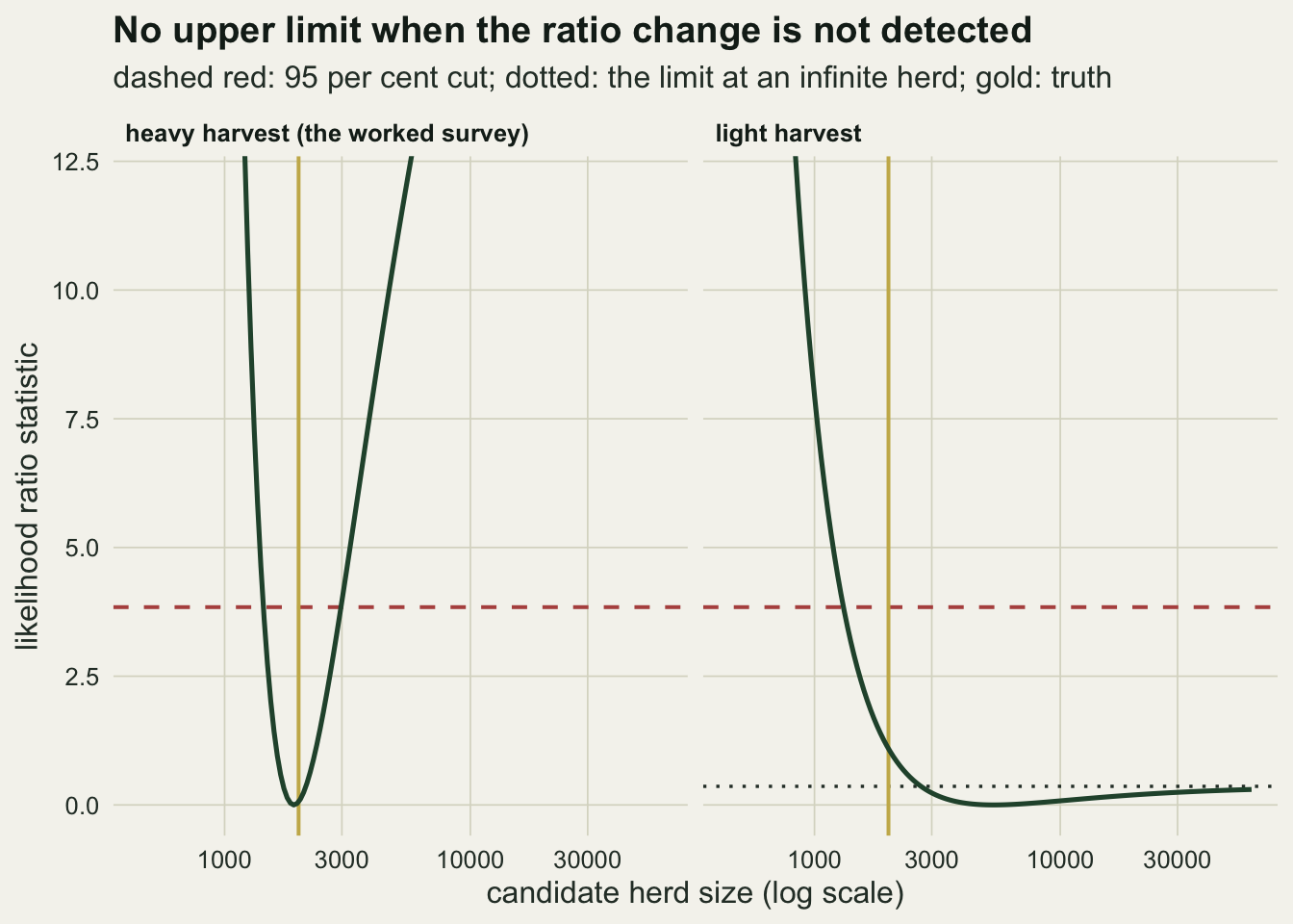
What to report
Report the two classified counts, the two sample sizes and the removals, not only the estimate. The estimate can be recomputed from those five numbers, and the reader can see at once how far apart the two proportions were.
Report the test that the ratio changed before the population estimate. If that test does not reject, the change-in-ratio survey has not measured population size and the estimate should not be printed as if it had. In the light season of this design that test, at the 5 per cent level, missed the change in 64 per cent of simulated seasons.
Give the profile likelihood interval, and give it with an open upper end when that is what it has. A Wald interval that runs below zero, or a percentile interval from a simulation whose tails are made of sign flips, puts a false floor and ceiling on a quantity the data did not bound.
Plan the harvest and the survey sizes together, before the season, from the delta method variance. Where the change is large enough to matter the formula gets the central spread right, and the ratio change in units of its own standard error tells in advance whether the season is likely to leave the estimator on the useful side of the curve. On this design, below 300 bucks from a herd of 2000 with 800 deer classified each time, the share of undefined or impossible estimates is at least one in a thousand.
Honest limits
The whole post assumes that males and females are equally likely to be seen and classified, in both surveys. That is the assumption that change-in-ratio methods are known to break in practice: males and females use different habitats and differ in how visible they are through the year, and a hunting season can change the behaviour of the survivors. A difference in detectability between the classes biases both proportions in a way that no amount of sample size corrects, and nothing simulated here measures it. Extensions exist that use two types of removal or more than two classes, but they bring their own assumptions.
The surveys are binomial. Sampling 800 animals without replacement from a herd of 2000 would be hypergeometric, with a smaller variance by a finite population factor.
fpc_before <- (herd_n - n_class) / (herd_n - 1)
fpc_after  <- (herd_n - rx_light - n_class) / (herd_n - rx_light - 1)
se_hyper   <- sqrt(p1_true * (1 - p1_true) / n_class * fpc_before +
                     p2_light * (1 - p2_light) / n_class * fpc_after)
se_ratio_hyper <- se_hyper / sd_change(rx_light)
n_hyp <- 5000
set.seed(6604)
y1_hyp <- rhyper(n_hyp, males_n, herd_n - males_n, n_class)
y2_hyp <- rhyper(n_hyp, males_n - rx_light, herd_n - males_n, n_class)
est_hyp <- cir_est(y1_hyp / n_class, y2_hyp / n_class, rx_light)
imp_hyp <- mean(!is.finite(est_hyp) | est_hyp < rx_light)
open_hyp <- mean(mapply(lr_at_infinity, y1_hyp, y2_hyp) < cut95)
In the light season the standard error of the proportion change would be 0.76 times the binomial one, the true change would sit 2.1 standard errors from zero instead of 1.6, and in 5000 simulated hypergeometric seasons 1.7 per cent of estimates are undefined or impossible, against 5.2 per cent under binomial surveys. The profile interval, which uses the binomial likelihood, does not gain from this: applied to the same hypergeometric counts it has no upper limit in 68.4 per cent of seasons; using the extra precision would need a likelihood written for sampling without replacement. The binomial model is the better description of a roadside count in which one deer can be seen twice, and the worse description of a complete classification of a fenced population.
The herd is closed apart from the harvest. Natural deaths, births and movement between the two surveys change both the total and the sex ratio and are indistinguishable from harvest in this estimator. The removals are taken as known without error, which registration stations approach for a legal harvest and nothing approaches for wounding loss or poaching.
The profile interval was calibrated against the chi squared cut, and its coverage was checked at two harvests only. The rule that it has no upper limit when the homogeneity test does not reject is exact, but whether the lower limit covers at the nominal rate in much smaller surveys, where the binomial counts are coarse, was not measured. Only a bucks-only season was simulated; a season that also removes females changes the numerator and the weight on the second survey, though not the square of the ratio change in the denominator.
References
Paulik GJ, Robson DS 1969 Journal of Wildlife Management 33(1):1-27 (10.2307/3799646)
Seber GAF 1982 The Estimation of Animal Abundance and Related Parameters, 2nd edition (Blackburn Press reprint 2002, ISBN 1-930665-55-5)
Fieller EC 1954 Journal of the Royal Statistical Society Series B 16(2):175-185 (10.1111/j.2517-6161.1954.tb00159.x)