library(ggplot2)

te_paper  <- "#f5f4ee"
te_ink    <- "#16241d"
te_body   <- "#2c3a31"
te_forest <- "#275139"
te_rust   <- "#b5534e"
te_gold   <- "#c9b458"
te_line   <- "#dad9ca"

theme_datasheet <- function() {
  theme_minimal(base_size = 12) +
    theme(plot.background  = element_rect(fill = te_paper, colour = NA),
          panel.background = element_rect(fill = te_paper, colour = NA),
          panel.grid.major = element_line(colour = te_line, linewidth = 0.3),
          panel.grid.minor = element_blank(),
          text             = element_text(colour = te_body),
          axis.text        = element_text(colour = te_body),
          strip.text       = element_text(colour = te_ink, face = "bold"))
}The delta method: standard errors for derived values
R
statistics
GLM
logistic regression
uncertainty
simulation
ecology tutorial
The delta method in R: a standard error for a species’ thermal optimum from glm() coefficients, and what dropping their covariance does to the interval.
A hundred and fifty plots spread over a region where mean annual temperature runs from 2 to 22 C, and in each plot a record of whether a grassland plant is present. You fit glm(pres ~ temp + I(temp^2), family = binomial), the squared term comes out negative, and the fitted curve has a hump. The species’ optimum, the temperature where the curve peaks, is -b1 / (2 * b2). summary() gives you a standard error for b1 and one for b2. What is the standard error of the optimum?
The optimum is a derived value: a function of fitted coefficients, not a coefficient itself. The delta method is the standard tool for its uncertainty, and many posts on this site use it in passing (for effective doses, return levels, occupancy). This post teaches it on the optimum: one line of algebra, a small helper that works for any derived value, a check that the helper is right, and the one trap in doing the calculation by hand from the summary() table.
The short answer. Write the derived value as a function g() of the coefficient vector. Its standard error is sqrt(t(grad) %*% vcov(fit) %*% grad), where grad holds the partial derivatives of g() with respect to each coefficient, evaluated at the estimates. Use the whole covariance matrix from vcov(), not only the standard errors on its diagonal: coefficients of temp and temp^2 are strongly correlated, and leaving that out can make the standard error several times too large. When the derived value is a ratio whose denominator is poorly determined, the symmetric interval from the delta method misses mostly on one side, and percentiles of the derived value computed from simulated coefficient vectors follow the skew better.
All data here are simulated, and every seed is in the code.
A humped response and its optimum
A logistic regression with a linear and a squared term, logit(p) = b0 + b1 * temp + b2 * temp^2, is the Gaussian logit response model of ter Braak and Looman (1986). When b2 is negative the curve has one peak. Its optimum is u = -b1 / (2 * b2), its tolerance (the width of the hump, like a standard deviation) is 1 / sqrt(-2 * b2), and the peak probability is plogis(b0 - b1^2 / (4 * b2)). The simulation starts from those three quantities, fixed before anything was run: optimum 14 C, tolerance 4 C, peak probability 0.8. Temperature is left in degrees Celsius, as most people would enter it.
opt_true  <- 14      # C
tol_true  <- 4       # C
peak_true <- 0.8
b2_true <- -1 / (2 * tol_true^2)
b1_true <- -2 * b2_true * opt_true
b0_true <- qlogis(peak_true) - (b1_true * opt_true + b2_true * opt_true^2)

simulate_plots <- function(n_plots) {
  temp <- runif(n_plots, 2, 22)
  data.frame(temp, pres = rbinom(n_plots, 1, plogis(b0_true + b1_true * temp + b2_true * temp^2)))
}

set.seed(1016)
plots <- simulate_plots(150)
fit   <- glm(pres ~ temp + I(temp^2), family = binomial, data = plots)
round(summary(fit)$coefficients, 4)
Estimate Std. Error z value Pr(>|z|)
(Intercept) -3.4121 0.9118 -3.7422 2e-04
temp 0.6895 0.1663 4.1450 0e+00
I(temp^2) -0.0255 0.0066 -3.8830 1e-04optimum <- function(b) unname(-b[2] / (2 * b[3]))
opt_hat <- optimum(coef(fit))
opt_hat[1] 13.52679The species was found in 89 of the 150 plots, and the fitted optimum is 13.53 C against the true 14. summary() has nothing to say about how certain that number is, because the optimum is not a row of its table.
The delta method in one line
If the estimates are close to the truth, a smooth function g() of them is close to a straight line in the coefficients, and a straight line of normally distributed estimates has a variance you can write down. The first-order Taylor approximation gives
Var(g(b_hat)) ~ t(grad) %*% V %*% gradwhere V is the covariance matrix of the coefficients (vcov(fit)) and grad is the vector of partial derivatives of g() with respect to b0, b1 and b2, evaluated at the estimates (Oehlert 1992; Ver Hoef 2012 traces who first published it). For the optimum -b1 / (2 * b2) the derivatives are 0 for b0, -1 / (2 * b2) for b1 and b1 / (2 * b2^2) for b2. Working out derivatives by hand is where mistakes creep in, so here is a helper that computes them numerically by central differences and works for any g(). Its step is a fixed fraction of each coefficient, because coefficients can be tiny (the squared term of an elevation in metres, say).
delta_se <- function(g, est, V, rel_step = 1e-5) {
  grad <- sapply(seq_along(est), function(j) {
    step <- if (est[j] != 0) rel_step * abs(est[j]) else rel_step
    up <- est; up[j] <- est[j] + step
    dn <- est; dn[j] <- est[j] - step
    (g(up) - g(dn)) / (2 * step)
  })
  sqrt(drop(t(grad) %*% V %*% grad))
}

se_opt <- delta_se(optimum, coef(fit), vcov(fit))

# the same with the derivatives written out
b_hat <- coef(fit); V_hat <- vcov(fit)
grad_opt <- c(0, -1 / (2 * b_hat[3]), b_hat[2] / (2 * b_hat[3]^2))
se_opt_analytic <- sqrt(drop(t(grad_opt) %*% V_hat %*% grad_opt))
c(numeric = se_opt, analytic = se_opt_analytic)
numeric analytic
0.6759742 0.6759742 # the helper works for any derived value
tolerance <- function(b) unname(1 / sqrt(-2 * b[3]))
c(tolerance = tolerance(coef(fit)), se = delta_se(tolerance, coef(fit), vcov(fit)))tolerance se
4.4292851 0.5703455 The numerical and the analytic gradient give the same standard error, 0.676 C, to a relative difference of \(2.1 \times 10^{-10}\). The 95 per cent interval for the optimum is the estimate plus or minus 1.96 standard errors: 12.20 to 14.85 C. The same helper, given a different g(), puts a standard error of 0.57 C on the tolerance of 4.43 C, and it would do the same for a peak probability, an LC50 or a population growth rate built from vital rates; Powell (2007) works through such demographic examples for field biologists.
The trap: two standard errors without their covariance
The tempting shortcut takes the two standard errors from summary() and combines them as if the estimates of b1 and b2 were independent: the same formula with only the diagonal of V. That is what a hand calculation from the coefficient table gives, since the table has no covariances in it.
ci_full <- opt_hat + c(-1, 1) * qnorm(0.975) * se_opt   # the interval with the covariance
se_diag <- sqrt(sum(grad_opt^2 * diag(V_hat)))
ci_diag <- opt_hat + c(-1, 1) * qnorm(0.975) * se_diag
round(c(full = se_opt, diagonal_only = se_diag, ratio = se_diag / se_opt), 3)
full diagonal_only ratio
0.676 4.773 7.062 round(cov2cor(V_hat), 3) # correlations between the coefficient estimates (Intercept) temp I(temp^2)
(Intercept) 1.000 -0.945 0.879
temp -0.945 1.000 -0.982
I(temp^2) 0.879 -0.982 1.000Leaving out the covariance makes the standard error 7.1 times too large here. The reason is in the correlation matrix: the estimates of b1 and b2 have a correlation of -0.982. With temperature running from 2 to 22 C, temp and temp^2 rise together across the plots, so a fit that tilts b1 up must bend b2 down to follow the data, and the optimum, their ratio, moves much less than either coefficient does. The diagonal-only formula throws that information away. The interval it reports for this survey runs from 4.2 to 22.9 C, from near the cold end of the sampled gradient to past its warm end:
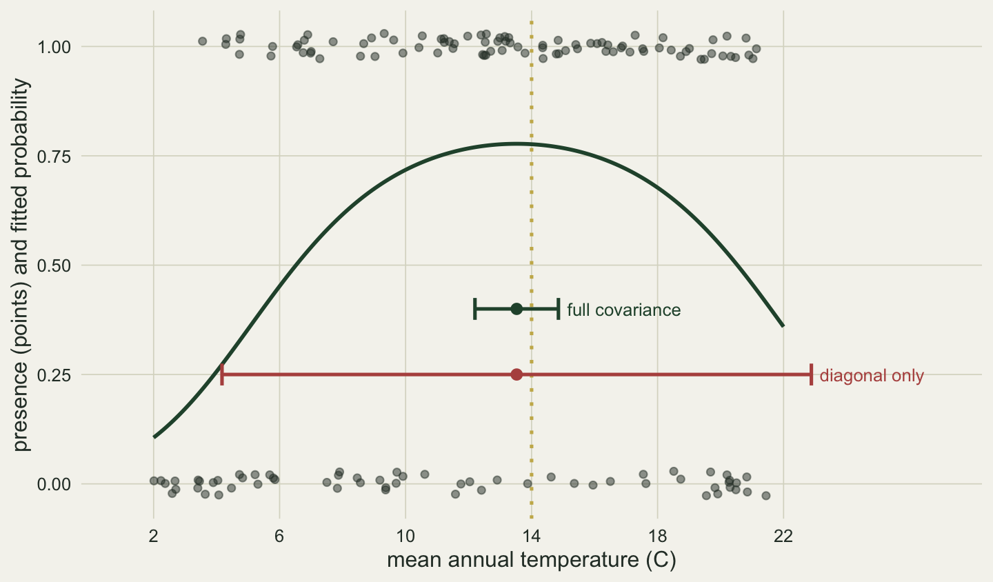
One survey shows the size of the error, not how often each interval covers the truth. For that, the survey is repeated with new plots at three sample sizes, and both intervals are computed from the same fit each time:
one_survey <- function(n_plots) {
  d  <- simulate_plots(n_plots)
  m  <- glm(pres ~ temp + I(temp^2), family = binomial, data = d)
  b  <- coef(m); V <- vcov(m)
  gr <- c(0, -1 / (2 * b[3]), b[2] / (2 * b[3]^2))
  # a percentile interval from 1000 simulated coefficient vectors (explained further down)
  b_sim <- MASS::mvrnorm(1000, b, V); q <- quantile(-b_sim[, 2] / (2 * b_sim[, 3]), c(0.025, 0.975))
  c(n = n_plots, opt = optimum(b), se_full = sqrt(drop(t(gr) %*% V %*% gr)),
    se_diag = sqrt(sum(gr^2 * diag(V))), cor_b1b2 = cov2cor(V)[2, 3],
    b2 = unname(b[3]), lo_sim = q[[1]], hi_sim = q[[2]], converged = m$converged)
}
n_rep <- 3000
set.seed(2016)
reps <- as.data.frame(do.call(rbind, lapply(c(60, 150, 400), function(n_plots)
  t(replicate(n_rep, one_survey(n_plots))))))

z95 <- qnorm(0.975)
reps$cover_full <- abs(reps$opt - opt_true) < z95 * reps$se_full
reps$cover_diag <- abs(reps$opt - opt_true) < z95 * reps$se_diag
cover_tab <- do.call(rbind, lapply(split(reps, reps$n), function(r) data.frame(
  n_plots = r$n[1], cover_full = mean(r$cover_full),
  mc_se = sqrt(mean(r$cover_full) * (1 - mean(r$cover_full)) / nrow(r)),
  cover_diag = mean(r$cover_diag), width_ratio = median(r$se_diag / r$se_full),
  cor_b1b2 = median(r$cor_b1b2))))
round(cover_tab, 3)
n_plots cover_full mc_se cover_diag width_ratio cor_b1b2
60 60 0.948 0.004 1 7.242 -0.984
150 150 0.956 0.004 1 7.180 -0.983
400 400 0.951 0.004 1 7.164 -0.983With the full covariance the interval covers the true optimum in 0.948 to 0.956 of the surveys, depending on the sample size, against the nominal 0.95 (one Monte Carlo standard error is about 0.004). At every sample size the share is within 1.7 standard errors of 0.95, but the total hides lopsided misses, shown in the section on the ratio below. The diagonal-only interval missed the truth in 0 of the 9000 surveys (by the rule of three, an approximate 95 per cent upper bound of 0.0003 on its miss rate). That is not a better interval: it covers everything because its median width is 7.16 to 7.24 times the width of the correct one, at every sample size. More plots shrink both standard errors but not the ratio between them, because the ratio is set by the correlation between the estimates of b1 and b2 (median -0.983 to -0.984 across the three designs), and that correlation depends on where the temperatures lie, not on how many plots there are.
Centring changes the parts, not the answer
If the correlation comes from temp and temp^2 rising together, subtracting the mean temperature before squaring should break it. It does, and it is worth seeing what it does and does not change:
temp_mean <- mean(plots$temp)
plots$temp_c <- plots$temp - temp_mean
fit_c <- glm(pres ~ temp_c + I(temp_c^2), family = binomial, data = plots)
b_c <- coef(fit_c); V_c <- vcov(fit_c)
grad_c <- c(0, -1 / (2 * b_c[3]), b_c[2] / (2 * b_c[3]^2))
se_full_c <- delta_se(optimum, b_c, V_c)
se_diag_c <- sqrt(sum(grad_c^2 * diag(V_c)))
cor_c <- cov2cor(V_c)[2, 3]
round(c(cor_b1b2_c = cor_c, optimum_c = optimum(b_c) + temp_mean,
        se_full_c = se_full_c, se_diag_c = se_diag_c), 4)
cor_b1b2_c optimum_c se_full_c se_diag_c
-0.0623 13.5268 0.6760 0.6938 On the centred scale the correlation between the two estimates is -0.062 instead of -0.982, and the diagonal-only standard error drops to 0.694 C, 1.03 times the full one. The fitted curve, the optimum (once the mean temperature of 12.29 C is added back) and the full delta standard error, 0.676 C, are the same as before. That is the point of this section: the two models are one model written in two codings, and the correct standard error cannot depend on the coding. Centring made the shortcut less wrong on this survey; it did not make the shortcut the method, and the correlation will not be this small in every data set. Use the full vcov() in either coding. (Centring has a real job when a penalty is involved, which is the subject of Centring a quadratic before lasso or ridge.)
Two formulas that are not what they look like
Centring is a coding that changes the parts and nothing else. Two other ways of writing the squared term look like codings too, and they are easy to type when a model is refitted from memory:
f_caret <- glm(pres ~ temp + temp^2, family = binomial, data = plots)             # no I()
f_poly  <- glm(pres ~ poly(temp, 2), family = binomial, data = plots)              # orthogonal basis
f_raw   <- glm(pres ~ poly(temp, 2, raw = TRUE), family = binomial, data = plots)  # plain powers
attr(terms(f_caret), "term.labels")   # the terms R actually fitted
[1] "temp"coding_fits <- list(f_caret, f_poly, f_raw)
coding_tab <- data.frame(formula = c("temp + temp^2", "poly(temp, 2)", "poly(temp, 2, raw = TRUE)"),
n_coef = sapply(coding_fits, function(m) length(coef(m))),
optimum = sapply(coding_fits, function(m) optimum(coef(m))),
delta_se = sapply(coding_fits, function(m) delta_se(optimum, coef(m), vcov(m))),
AIC = sapply(coding_fits, AIC))
print(coding_tab, digits = 4) formula n_coef optimum delta_se AIC
1 temp + temp^2 2 NA NA 201.4
2 poly(temp, 2) 3 0.2857 0.1325 186.5
3 poly(temp, 2, raw = TRUE) 3 13.5268 0.6760 186.5The first formula runs without an error or a warning, and it is not a quadratic. In a model formula ^ means crossing, not a power: (a + b)^2 asks for both main effects and their interaction, and temp crossed with itself is just temp. The model has 2 coefficients, exactly those of glm(pres ~ temp). Its summary() shows a positive slope for temperature with p = 0.024, which read on its own says the plant favours warm plots, and its AIC is 201.39 against 186.52 for the humped model. The optimum comes back NA, because there is no third coefficient to divide by. I(temp^2) is what keeps the arithmetic away from the formula algebra.
The orthogonal polynomial is the same model: its fitted probabilities equal those of fit at every plot. Its coefficients are not b0, b1 and b2, though. The first column of poly() is the centred temperature of the section above, rescaled to unit length, and the second is a quadratic made orthogonal to the first and to the intercept, also of unit length, both built from this survey’s own mean (12.29 C) and spread. Put these coefficients into -b1 / (2 * b2) and the “optimum” is 0.29, which read as a temperature lies below the coldest plot at 2.01 C. It is not a temperature. Worked through the basis, the formula returns k * (u - c): the optimum u of the fitted curve shifted by c = 12.07 C (the average of the two centring constants poly() stored) and multiplied by k = 0.196 per C (the ratio of the lengths of the two basis columns before poly() scaled them to unit length), so on this survey’s basis any optimum from 2 to 22 C lands between -2.0 and 1.9. delta_se() gives it a standard error of 0.133, the correct 0.676 C times the same k: the uncertainty is right, the scale is foreign, and nothing in the output says so. Every step runs and the result looks like a temperature with a tight interval, which makes this the more dangerous of the two. With raw = TRUE, poly() returns the plain powers, the coefficients equal those of fit, and the optimum and its standard error are the ones found earlier, 13.53 and 0.676 C.
A check that does not depend on the coding reads the optimum off the fitted curve. predict() rebuilds the orthogonal basis for new temperatures from what the model stored, so this works for f_poly as well as for fit:
opt_curve <- optimize(function(x) predict(f_poly, data.frame(temp = x)), c(2, 22), maximum = TRUE)$maximum
c(from_curve = opt_curve, from_fit = opt_hat)
from_curve from_fit
13.52679 13.52679 stopifnot(abs(opt_curve - opt_hat) < 1e-3)It returns 13.53 C, the optimum of fit to the tolerance of optimize(). Species distribution modelling with GLM in R reads the peak of its poly() fits the same way, from a grid of predictions. The curve gives the optimum but not its standard error: for that, refit with I(temp^2) or raw = TRUE and use delta_se(), or resample the plots and read the curve again each time (a bootstrap, not shown here).
When the ratio misbehaves
The delta method replaces g() by a straight line, and the optimum is a ratio. When the denominator, the curvature b2, is estimated well, a straight line is a good approximation, and the two-sided coverage in the coverage table above is close to 0.95. When b2 is poorly determined, small changes in it move the optimum a long way in one direction and a short way in the other. The replicate surveys show it:
tail_tab <- do.call(rbind, lapply(split(reps, reps$n), function(r) {
  q <- quantile(r$opt, c(0.025, 0.975))
  data.frame(n_plots = r$n[1], median_se = median(r$se_full), sd_opt = sd(r$opt),
             below = opt_true - q[[1]], above = q[[2]] - opt_true,
             miss_low = mean(r$opt + z95 * r$se_full < opt_true),
             miss_high = mean(r$opt - z95 * r$se_full > opt_true))
}))
round(tail_tab, 3)
n_plots median_se sd_opt below above miss_low miss_high
60 60 0.927 5.589 1.626 4.202 0.052 0.001
150 150 0.595 0.698 1.051 1.675 0.041 0.003
400 400 0.366 0.392 0.692 0.868 0.040 0.009At 60 plots the standard deviation of the 3000 estimated optima is 5.59 C, while the median delta standard error is 0.93 C. The standard deviation is driven by a few surveys: in 3 of them b2 came out zero or positive, so the curve had no hump at all, and in others it was only slightly negative, which puts the “optimum” far from the true 14 C; 41 of the 3000 estimates lie outside 11 to 21 C, and without those the standard deviation is 1.18 C. The percentiles tell the shape better. The 2.5th percentile of the estimates lies 1.63 C below the true optimum and the 97.5th lies 4.20 C above it, while the delta interval reaches the same distance, about 1.82 C at the median standard error, on both sides. The coverage stayed near 0.95, but the misses are lopsided, where a symmetric interval should put 0.025 on each side: 0.052 of the intervals fell entirely below the truth and 0.001 entirely above it.
The misses sit on the cold side, opposite to the long warm tail, because the standard error moves with the estimate. The gradient of the optimum has b2 in its denominator, so a flatter fitted curve (b2 closer to zero) gets a larger standard error, and flatter curves also tend to put the optimum on the warm side. A warm estimate therefore carries a wide interval that still reaches back to 14 C, while a cold estimate from a sharp hump gets a narrow interval that can stop short of it. At 60 plots the median standard error is 0.77 C for estimates below 14 C and 1.23 C for those above; an interval of one fixed width (the median standard error) would have missed 0.014 below and 0.086 above, mostly on the warm side. The total coverage is what is left after the two sides trade off: at 150 plots 0.003 of the intervals missed on the warm side and 0.041 on the cold side, 0.044 in all against the nominal 0.05. With more plots the tails shrink and even out, 0.69 C below and 0.87 C above at 400 plots, but the misses there are still 0.040 below and 0.009 above.
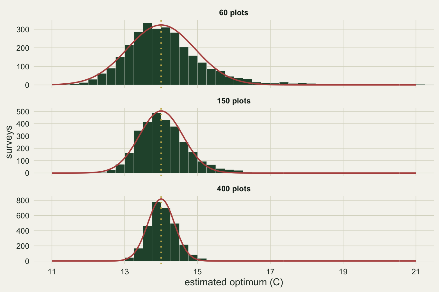
A symmetric interval centred on the estimate cannot follow this. The better intervals for a ratio of coefficients, Fieller’s interval and the profile likelihood interval, are compared with the delta interval in Confidence intervals for effective doses; Maximum likelihood by hand with optim() in R shows how to profile a parameter; and Return levels and uncertainty shows the same failure for a high quantile of an extreme value fit, where the delta interval is too short on the upper side.
The same fitted model gives a second route to an interval, without any derivatives: draw many coefficient vectors from a multivariate normal distribution with mean coef(fit) and covariance vcov(fit), compute the optimum for each, and read off percentiles. MASS::mvrnorm() does the drawing. Here it is for the one survey of 150 plots, and then for the replicate surveys, where one_survey() already drew 1000 coefficient vectors per fit:
set.seed(3016)
coef_draws <- MASS::mvrnorm(10000, mu = coef(fit), Sigma = vcov(fit))
opt_draws  <- apply(coef_draws, 1, optimum)
round(rbind(delta_interval = ci_full, simulated = quantile(opt_draws, c(0.025, 0.975))), 2)
2.5% 97.5%
delta_interval 12.20 14.85
simulated 12.31 15.42c(sd_of_draws = sd(opt_draws), delta_se = se_opt)sd_of_draws delta_se
7.3448119 0.6759742 sim_tab <- sapply(split(reps, reps$n), function(r) c(miss_low = mean(r$hi_sim < opt_true),
miss_high = mean(r$lo_sim > opt_true), cover = mean(r$lo_sim < opt_true & r$hi_sim > opt_true)))
round(sim_tab, 3) # percentile intervals in the replicate surveys, columns = plots 60 150 400
miss_low 0.023 0.020 0.03
miss_high 0.004 0.023 0.03
cover 0.973 0.957 0.94The percentile interval for the one survey runs from 12.31 to 15.42 C, against 12.20 to 14.85 C from the delta method: a lower end 0.11 C higher and an upper end 0.57 C higher, the same warm lean as in the replicate surveys. Read percentiles, not the standard deviation of the draws: one draw of the 10000 had b2 practically zero and an optimum of 743 C, which inflates the standard deviation to 7.34 C (0.85 C without it) but moves a percentile by at most one place in the sorted draws. Over the replicate surveys the percentile interval spreads its misses more evenly than the delta interval at 150 and 400 plots (0.020 below and 0.023 above at 150, 0.030 and 0.030 at 400), with coverage 0.957 and 0.940. At 60 plots it covers 0.973 and still misses more often on the cold side (0.023 below, 0.004 above), though less often than the delta interval did. It follows the skew better; it is not exact either.
All of this has the optimum well inside the gradient. The usual sample-size check for a logistic regression is the rule of at least 10 events per variable (EPV) from the simulations of Peduzzi et al. (1996); events are the rarer outcome, and here the variables are the two slope coefficients, of temp and temp^2. The chunk below keeps the tolerance of 4 C and the peak probability of 0.8, sets the number of plots so that the rarer outcome is expected in 20 or 80 of them (EPV 10 or 40 at the expected prevalence; epv_seen is the average realised EPV), and moves the optimum from 14 C to 20 C, 2 C from the warm end of the sampled gradient. Beside the delta interval it computes Fieller’s set for the optimum, the same construction as for the effective doses: b1 + 2 * u * b2 is zero at the optimum u, so the set holds every u for which (b1 + 2 * u * b2)^2 <= 1.96^2 * (v11 + 4 * u * v12 + 4 * u^2 * v22), with v the entries of vcov() for b1 and b2. That is a quadratic inequality in u, and when b2 cannot be told from zero its solution is not a bounded interval.
edge_design <- function(u, epv) {   # host tolerance and peak, optimum u, plots set by the expected EPV
  b2 <- -1 / (2 * tol_true^2); b1 <- -2 * b2 * u; b0 <- qlogis(peak_true) - (b1 * u + b2 * u^2)
  prev <- integrate(function(x) plogis(b0 + b1 * x + b2 * x^2), 2, 22)$value / 20
  c(opt = u, epv = epv, plots = ceiling(2 * epv / min(prev, 1 - prev)), b0 = b0, b1 = b1, b2 = b2)
}
edge_survey <- function(d) {
  temp <- runif(d[["plots"]], 2, 22); warned <- FALSE
  pres <- rbinom(d[["plots"]], 1, plogis(d[["b0"]] + d[["b1"]] * temp + d[["b2"]] * temp^2))
  m <- withCallingHandlers(glm(pres ~ temp + I(temp^2), family = binomial),   # count the 0-or-1 warning, do not print it
    warning = function(w) { stopifnot(grepl("0 or 1", conditionMessage(w))); warned <<- TRUE; invokeRestart("muffleWarning") })
  b <- unname(coef(m)); V <- vcov(m); u <- d[["opt"]]; o <- optimum(b)
  gr <- c(0, -1 / (2 * b[3]), b[2] / (2 * b[3]^2)); se <- sqrt(drop(t(gr) %*% V %*% gr))
  c(epv_seen = min(sum(pres), sum(1 - pres)) / 2, warned = warned, converged = m$converged,
    wald_b1 = abs(b[2] - d[["b1"]]) < z95 * sqrt(V[2, 2]), wald_b2 = abs(b[3] - d[["b2"]]) < z95 * sqrt(V[3, 3]),
    delta = abs(o - u) < z95 * se, delta_low = o + z95 * se < u, delta_high = o - z95 * se > u,
    fieller = (b[2] + 2 * u * b[3])^2 <= z95^2 * (V[2, 2] + 4 * u * V[2, 3] + 4 * u^2 * V[3, 3]),
    bounded = b[3]^2 > z95^2 * V[3, 3], nohump = b[3] >= 0, outside = b[3] < 0 && (o < 2 || o > 22))   # bounded: u^2 term > 0
}
n_epv <- 2000; set.seed(4016); epv_tab <- t(sapply(list(edge_design(14, 10), edge_design(20, 10), edge_design(20, 40)), function(d)
  c(d[c("opt", "epv", "plots")], colMeans(t(replicate(n_epv, edge_survey(d)))))))
round(epv_tab, 3)
opt epv plots epv_seen warned converged wald_b1 wald_b2 delta delta_low
[1,] 14 10 46 9.661 0.000 1 0.970 0.970 0.948 0.052
[2,] 20 10 53 10.003 0.021 1 0.952 0.957 0.824 0.176
[3,] 20 40 211 40.103 0.000 1 0.957 0.959 0.889 0.110
delta_high fieller bounded nohump outside
[1,] 0.001 0.958 0.744 0.004 0.012
[2,] 0.000 0.966 0.162 0.080 0.271
[3,] 0.000 0.962 0.769 0.002 0.212The rule does what it was built for: the Wald intervals for b1 and b2 cover their true values in 0.952 to 0.970 of the 2000 surveys per design, edge or not, and with the optimum at 14 C, EPV 10 (46 plots) gives the delta interval for the optimum a coverage of 0.948. With the optimum at 20 C the same EPV (53 plots) gives 0.824 (Monte Carlo standard error 0.009), every miss an interval that ends below 20 C, as most misses at 14 C did (0.052 below, 0.001 above), the cold-side lean of the 60-plot surveys above; four times the events (211 plots) raise it only to 0.889. The estimated optimum lay outside the sampled 2 to 22 C in 0.271 of the edge surveys at EPV 10 and 0.212 at EPV 40; in a further 0.080 at EPV 10 b2 came out zero or positive, with no hump at all, and glm() warned of fitted probabilities of 0 or 1 in 0.021; every column counts both kinds of fit. Fieller’s set covers the true optimum in 0.958 to 0.966 of the surveys in every design, but read that as Confidence intervals for effective doses reads its very narrow layout: at the edge with EPV 10 only 0.162 of the sets were a bounded interval (0.769 at EPV 40), and the rest were unbounded (every temperature outside one stretch, or every temperature). Such a set can rule out a stretch but does not pin the optimum to one, so its coverage says little; it is a more honest answer than a delta interval that misses, not a narrower one. EPV protects the coefficients; it says nothing about a ratio of them near the edge of the design.
What to check in your own data
Check that your derived value uses vcov(fit) and not sqrt(diag(vcov(fit))). If you are copying numbers from a summary() table into a calculator or a spreadsheet, you are almost certainly leaving out the covariance. Check that a model with a squared term has three coefficients: temp^2 without I() fits a straight line, and coefficients from poly() without raw = TRUE do not go into -b1 / (2 * b2).
Check your gradient before you trust it. Compute the standard error with the numerical helper and with the derivatives you wrote out; if they differ beyond the fifth or sixth digit, one of them is wrong: check the step size of the numerical one and your algebra.
Look at the estimate of the denominator of any ratio you report. For an optimum, a curvature b2 whose interval comes close to zero means the data barely show a hump, and the optimum can then lie anywhere; report that, and the profile or simulated interval, rather than a symmetric one. If the optimum sits near the end of your sampled gradient (the 20 C design above, where every delta miss fell on the cold side and 0.271 of the estimates at EPV 10 lay outside the gradient), expect a more lopsided sampling distribution, because the curve is only seen falling on one side. Draw coefficient vectors as in the MASS::mvrnorm() chunk above and look at the histogram of the derived value before you report plus or minus 1.96 standard errors.
Honest limits
The simulation uses one species: an optimum at 14 C (20 C, near the warm end, only in the events-per-variable check), a tolerance of 4 C, a peak probability of 0.8 and plots spread evenly from 2 to 22 C. The size of the diagonal-only error depends on the correlation between the coefficient estimates, and so on where the temperatures lie: centring made the shortcut look harmless on this survey. The coverage study counts every fit, including the 3 at 60 plots with no hump and 0.080 of the edge surveys at EPV 10, from which a real analysis would not report an optimum. The delta method is also only as good as vcov(): with overdispersed or spatially correlated presence data the covariance matrix is too small, and the delta standard error inherits that.
References
Oehlert GW 1992 The American Statistician 46(1):27-29 (10.1080/00031305.1992.10475842)
Peduzzi P, Concato J, Kemper E, Holford TR, Feinstein AR 1996 Journal of Clinical Epidemiology 49(12):1373-1379 (10.1016/S0895-4356(96)00236-3)
Powell LA 2007 The Condor 109(4):949-954 (10.1093/condor/109.4.949)
ter Braak CJF, Looman CWN 1986 Vegetatio 65(1):3-11 (10.1007/BF00032121)
Ver Hoef JM 2012 The American Statistician 66(2):124-127 (10.1080/00031305.2012.687494)