library(ggplot2)

te_paper  <- "#f5f4ee"
te_ink    <- "#16241d"
te_body   <- "#2c3a31"
te_forest <- "#275139"
te_rust   <- "#b5534e"
te_gold   <- "#c9b458"
te_line   <- "#dad9ca"

theme_datasheet <- function() {
  theme_minimal(base_size = 12) +
    theme(plot.background  = element_rect(fill = te_paper, colour = NA),
          panel.background = element_rect(fill = te_paper, colour = NA),
          panel.grid.major = element_line(colour = te_line, linewidth = 0.3),
          panel.grid.minor = element_blank(),
          text             = element_text(colour = te_body),
          plot.title       = element_text(colour = te_ink, face = "bold"),
          plot.subtitle    = element_text(colour = te_body),
          axis.text        = element_text(colour = te_body),
          strip.text       = element_text(colour = te_ink))
}Global sensitivity analysis with Sobol indices
R
sensitivity analysis
uncertainty
matrix models
fisheries
simulation
ecology tutorial
Sobol indices by hand in R for a stage matrix and a harvest model: when they only repeat elasticity times input spread, and where interaction sets them apart.
A population model for a long-lived species has five vital rates, and they are not known equally well. Adult survival comes from years of resighting marked adults and is pinned between 0.85 and 0.95. Juvenile survival, the first years away from the breeding site, is barely known: anything from 0.1 to 0.5 fits what little data there are. The model returns the growth rate lambda, and the question for the next field season is which rate’s uncertainty matters for lambda, that is, where better data would change the answer most.
The usual first tool is elasticity, and this site has it for matrix models and for integral projection models. Both posts compute proportional slopes of lambda at one parameter set and read them as a priority list for management; neither asks how far each rate can actually move. That is a local answer to a global question. Mills, Doak and Wisdom (1999) showed with three real data sets that recommendations built on elasticities can mislead when the rates vary by different amounts, and suggested simulating over the range of each rate instead. The variance-based indices of Sobol (2001) are the general form of that simulation: the share of the variance of the output that each input explains on its own, and the share it takes part in once its interactions with the other inputs are counted.
Checking a reintroduction analysis does a split of the same kind at the level of sources rather than inputs: it switches demographic stochasticity, environmental stochasticity and parameter uncertainty on one at a time, finds that the three parts do not add up to the whole, and calls its decomposition an accounting device rather than an identity. The Sobol total index is the construction that puts a number on that non-additivity, one input at a time. When a single model run is expensive, the thousands of runs an index needs are out of reach, and an emulator is the usual way round that; here both models run in microseconds.
Nothing below is new about the indices themselves. The estimators are the ones Saltelli and colleagues (2010) recommend, the first-order estimator from that paper and the total-effect estimator of Jansen (1999), coded by hand from their definitions. What the post measures is when the indices say something that elasticities and input ranges had not already said. A first-order Taylor expansion, the same expansion as the delta method, predicts each input’s share from its elasticity and the spread of its range alone. That share is computed first in every section, before any Sobol index, and the indices are then read against it.
Two indices from one set of runs
Write the model as Y = f(X_1, …, X_p) with independent inputs. The first-order index of input i is S_i = Var(E[Y | X_i]) / Var(Y): the share of the output variance that would go if X_i alone were fixed at its true value, averaged over where that value might be. The total index is ST_i = E[Var(Y | X_~i)] / Var(Y), where X_~i is every input except i: the share that would remain if everything but X_i were fixed. The total index includes every interaction X_i takes part in, so ST_i - S_i is the part of input i’s influence that depends on the values of the other inputs. For an additive model the two are equal and sum to one over the inputs.
Both come from one design. Draw two independent matrices A and B of N rows, one column per input. For input i, the matrix AB_i is A with its column i taken from B. With f(A), f(B) and f(AB_i) the model outputs row by row, Saltelli and colleagues (2010) estimate the first-order variance as mean(f(B) * (f(AB_i) - f(A))) and, following Jansen (1999), the total variance as mean((f(A) - f(AB_i))^2) / 2; both are divided by the variance of all the outputs in A and B. The cost is N times (p + 2) model runs. The function below also returns a centred version of the first-order estimate, which subtracts the output mean from f(B); the reason is a section further down.
A second, independent estimate of the first-order index needs no special design at all: cut one input into 100 classes of equal count, and take the share of the output’s sum of squares that lies between the class means. That is eta squared, the same statistic that the geographical detector calls q, applied with fine classes to one input at a time. With 100 classes it is biased upwards by roughly 99 / N when the input has no effect, which is negligible at the sample sizes used here.
draw_unif <- function(n, lo, hi) {
  x <- sapply(seq_along(lo), function(i) runif(n, lo[i], hi[i]))
  colnames(x) <- names(lo)
  x
}

sobol_run <- function(f, lo, hi, n_base, groups = as.list(seq_along(lo))) {
  a_mat <- draw_unif(n_base, lo, hi)
  b_mat <- draw_unif(n_base, lo, hi)
  f_a <- f(a_mat)
  f_b <- f(b_mat)
  v_y <- var(c(f_a, f_b))
  m_y <- mean(c(f_a, f_b))
  out <- t(sapply(groups, function(u) {
    ab_mat <- a_mat
    ab_mat[, u] <- b_mat[, u]
    f_ab <- f(ab_mat)
    c(S_raw = mean(f_b * (f_ab - f_a)) / v_y,
      S_cen = mean((f_b - m_y) * (f_ab - f_a)) / v_y,
      ST    = 0.5 * mean((f_a - f_ab)^2) / v_y,
      shift = m_y * mean(f_ab - f_a) / v_y)
  }))
  rownames(out) <- sapply(groups, function(u) paste(names(lo)[u], collapse = ":"))
  out
}

eta_sq <- function(f, lo, hi, n_draw, n_class = 100) {
  x <- draw_unif(n_draw, lo, hi)
  y <- f(x)
  tss <- sum((y - mean(y))^2)
  setNames(sapply(seq_along(lo), function(i) {
    cls <- cut(x[, i], quantile(x[, i], 0:n_class / n_class), include.lowest = TRUE)
    n_c <- tabulate(cls)
    (sum(rowsum(y, cls)^2 / n_c) - length(y) * mean(y)^2) / tss
  }), names(lo))
}

f_test <- function(x) x[, 1] + x[, 2] + 2 * x[, 1] * x[, 2]
lo_t <- c(x1 = -1, x2 = -1)
hi_t <- c(x1 = 1, x2 = 1)
v_one <- 1 / 3
v_int <- 4 * (1 / 3)^2
exact_S  <- v_one / (2 * v_one + v_int)
exact_ST <- (v_one + v_int) / (2 * v_one + v_int)

set.seed(5101)
chk <- sobol_run(f_test, lo_t, hi_t, 2e5)
chk_eta <- eta_sq(f_test, lo_t, hi_t, 2e5)
chk_err <- max(abs(c(chk[, "S_raw"] - exact_S, chk[, "S_cen"] - exact_S,
                     chk_eta - exact_S, chk[, "ST"] - exact_ST)))
stopifnot(chk_err < 0.01)
The check uses a function whose indices can be written down. With X_1 and X_2 uniform on -1 to 1, each has variance 1/3, the model Y = X_1 + X_2 + 2 X_1 X_2 has E[Y | X_1] = X_1, and the product term contributes a variance of 4/9 that belongs to neither input alone. So each first-order index is 0.3 and each total index 0.7. At N = 200 000 the four estimates (uncentred, centred and eta squared first-order, and the total index) land within 0.0038 of those values.
A stage matrix with one poorly known rate
The life cycle has juveniles, subadults and adults. Juveniles survive to become subadults with probability sj; subadults survive with probability ss and, if they survive, recruit to the adult stage with probability g; adults survive with probability sa and produce f female offspring each, counted at the next census, so the fecundity entry is f times sa. The ranges are the ones in the opening plus 0.6 to 0.8 for ss, 0.3 to 0.5 for g and 1.5 to 2.5 for f. They are illustrative, not taken from one species, and every range is uniform.
Lambda is the largest root of the characteristic polynomial of this matrix, which works out as lambda (lambda - ss (1 - g)) (lambda - sa) = f sa sj ss g. Newton’s method on that cubic, started above the root, gives lambda for a whole matrix of draws at once, and the chunk checks it against eigen().
The Taylor share comes next, before anything else. Expanding lambda to first order around the midpoints of the ranges, Var(lambda) / lambda^2 is approximately the sum over rates of (e_i CV_i)^2, where e_i is the elasticity of lambda to rate i and CV_i is that rate’s coefficient of variation over its range. For a uniform range from lo to hi the standard deviation is (hi - lo) / sqrt(12), so CV_i = (hi - lo) / (sqrt(12) * (lo + hi) / 2). The predicted share of each rate is its term divided by the sum. The elasticities are to the vital rates themselves rather than to the matrix entries, what Caswell (2001) calls lower-level parameters, and they are computed as central differences of log lambda at the midpoints.
lam_fast <- function(x) {
  a_sub <- x[, "ss"] * (1 - x[, "g"])
  s_ad  <- x[, "sa"]
  k_c   <- x[, "f"] * x[, "sa"] * x[, "sj"] * x[, "ss"] * x[, "g"]
  l_val <- rep(3, nrow(x))
  for (k in 1:40) {
    p_val <- l_val * (l_val - a_sub) * (l_val - s_ad) - k_c
    d_val <- 3 * l_val^2 - 2 * l_val * (a_sub + s_ad) + a_sub * s_ad
    l_val <- l_val - p_val / d_val
  }
  l_val
}
proj_mat <- function(v) matrix(c(0, 0, v[["f"]] * v[["sa"]],
                                 v[["sj"]], v[["ss"]] * (1 - v[["g"]]), 0,
                                 0, v[["ss"]] * v[["g"]], v[["sa"]]), 3, 3, byrow = TRUE)

lo_m <- c(sj = 0.1, ss = 0.6, g = 0.3, sa = 0.85, f = 1.5)
hi_m <- c(sj = 0.5, ss = 0.8, g = 0.5, sa = 0.95, f = 2.5)
nom_m <- (lo_m + hi_m) / 2

set.seed(5102)
x_chk <- draw_unif(300, lo_m, hi_m)
lam_err <- max(abs(lam_fast(x_chk) - apply(x_chk, 1, function(v)
  max(Re(eigen(proj_mat(v), only.values = TRUE)$values)))))
stopifnot(lam_err < 1e-10)

elast_fd <- function(f, nom, h = 1e-4) sapply(seq_along(nom), function(i) {
  up <- dn <- nom
  up[i] <- nom[i] * (1 + h)
  dn[i] <- nom[i] * (1 - h)
  x_two <- rbind(up, dn)
  colnames(x_two) <- names(nom)
  l_two <- log(f(x_two))
  (l_two[1] - l_two[2]) / (log(1 + h) - log(1 - h))
})
el_m  <- setNames(elast_fd(lam_fast, nom_m), names(nom_m))
cv_m  <- (hi_m - lo_m) / (sqrt(12) * nom_m)
tay_m <- (el_m * cv_m)^2 / sum((el_m * cv_m)^2)
lam_nom <- lam_fast(t(nom_m))

x_cv <- draw_unif(1e5, lo_m, hi_m)
cv_emp <- apply(x_cv, 2, sd) / colMeans(x_cv)
stopifnot(max(abs(cv_emp / cv_m - 1)) < 0.01)
print(round(rbind(elasticity = el_m, input_cv = cv_m, taylor_share = tay_m), 3))
sj ss g sa f
elasticity 0.124 0.200 0.073 0.676 0.124
input_cv 0.385 0.082 0.144 0.032 0.144
taylor_share 0.659 0.079 0.032 0.137 0.093The Newton solution matches eigen() to within \(4.4 \times 10^{-16}\) over 300 random matrices, and lambda at the midpoints is 1.101. The formula CVs agree with the sample CVs of 100 000 uniform draws to within one per cent (the stopifnot line).
Elasticity ranks adult survival first by a wide margin, 0.676, with subadult survival at 0.200 and juvenile survival at 0.124, the same value as fecundity. The Taylor share turns that round: juvenile survival takes 0.659 of the predicted variance and adult survival 0.137. The reversal is arithmetic in the inputs. The CV of juvenile survival over its range is 0.385 and that of adult survival 0.032, 12 times smaller. Squared, the CV ratio is 144, against 30 for the squared ratio of the elasticities the other way, and no Sobol index was needed to see it.
The indices repeat the arithmetic
The Sobol analysis uses N = 8000 rows per run, which costs 56000 evaluations of lambda for five rates, and the whole run is repeated 200 times with fresh draws, so that each index comes with its spread over replicates. The eta squared estimate uses five fresh samples of 200 000.
n_base <- 8000
n_rep  <- 200
set.seed(5103)
rep_m  <- replicate(n_rep, sobol_run(lam_fast, lo_m, hi_m, n_base))
mean_m <- apply(rep_m, 1:2, mean)
sd_m   <- apply(rep_m, 1:2, sd)
set.seed(5104)
eta_m_rep <- replicate(5, eta_sq(lam_fast, lo_m, hi_m, 2e5))
eta_m <- rowMeans(eta_m_rep)

gap_m <- mean_m[, "ST"] - tay_m
gap_max_m <- max(abs(gap_m))
gap_rate  <- names(which.max(abs(gap_m)))
mcse_st_m <- max(sd_m[, "ST"]) / sqrt(n_rep)
eta_gap_m <- max(abs(mean_m[, "S_cen"] - eta_m))
sum_s_m   <- sum(mean_m[, "S_cen"])
stopifnot(identical(order(mean_m[, "ST"]), order(tay_m)))
print(round(cbind(taylor = tay_m, S_centred = mean_m[, "S_cen"], eta_sq = eta_m,
                  ST = mean_m[, "ST"], sd_ST = sd_m[, "ST"]), 3))
taylor S_centred eta_sq ST sd_ST
sj 0.659 0.671 0.671 0.680 0.010
ss 0.079 0.071 0.073 0.074 0.001
g 0.032 0.030 0.030 0.032 0.001
sa 0.137 0.135 0.136 0.135 0.002
f 0.093 0.084 0.085 0.089 0.002Averaged over the 200 replicates, the total index of every rate lies within 0.021 of its Taylor share, the largest gap being juvenile survival at 0.680 against 0.659; the Monte Carlo standard error of each averaged total index is at most 0.0007, so that gap is real but small. The two first-order estimates, the centred pick-freeze one and eta squared, agree to within 0.002 on every rate, and the first-order indices sum to 0.990 (0.994 by eta squared): almost no variance in lambda over these ranges is interaction. The ranking by total index, juvenile survival first at 0.68 and adult survival second at 0.13, is the ranking the Taylor share gave from 10 evaluations of lambda around the midpoints.
rate_lab <- c(sj = "juvenile survival", ss = "subadult survival", g = "recruitment",
              sa = "adult survival", f = "fecundity")
mat_long <- rbind(
  data.frame(panel = "elasticity at the midpoints", rate = names(el_m),
             measure = "elasticity", val = el_m),
  data.frame(panel = "share of the variance of lambda", rate = names(tay_m),
             measure = "Taylor share", val = tay_m),
  data.frame(panel = "share of the variance of lambda", rate = rownames(mean_m),
             measure = "first-order S", val = mean_m[, "S_cen"]),
  data.frame(panel = "share of the variance of lambda", rate = rownames(mean_m),
             measure = "total ST", val = mean_m[, "ST"]))
mat_long$rate <- factor(rate_lab[mat_long$rate], rev(rate_lab[c("sa", "ss", "sj", "f", "g")]))
mat_long$measure <- factor(mat_long$measure,
                           c("elasticity", "Taylor share", "first-order S", "total ST"))
mat_long$panel <- factor(mat_long$panel, c("elasticity at the midpoints",
                                           "share of the variance of lambda"))
off_meas <- c("elasticity" = 0, "Taylor share" = -0.2, "first-order S" = 0, "total ST" = 0.2)
mat_long$y_pos <- as.numeric(mat_long$rate) + off_meas[as.character(mat_long$measure)]
ggplot(mat_long, aes(val, y_pos, colour = measure, shape = measure)) +
  geom_point(size = 3, stroke = 1.1) +
  facet_wrap(~ panel, scales = "free_x") +
  expand_limits(x = 0) +
  scale_y_continuous(breaks = seq_along(levels(mat_long$rate)), labels = levels(mat_long$rate)) +
  scale_colour_manual(values = c(te_ink, te_gold, te_forest, te_rust), name = NULL) +
  scale_shape_manual(values = c(16, 18, 1, 4), name = NULL) +
  labs(x = NULL, y = NULL,
       title = "Elasticity ranks adult survival first; the variance does not") +
  theme_datasheet() +
  theme(legend.position = "bottom")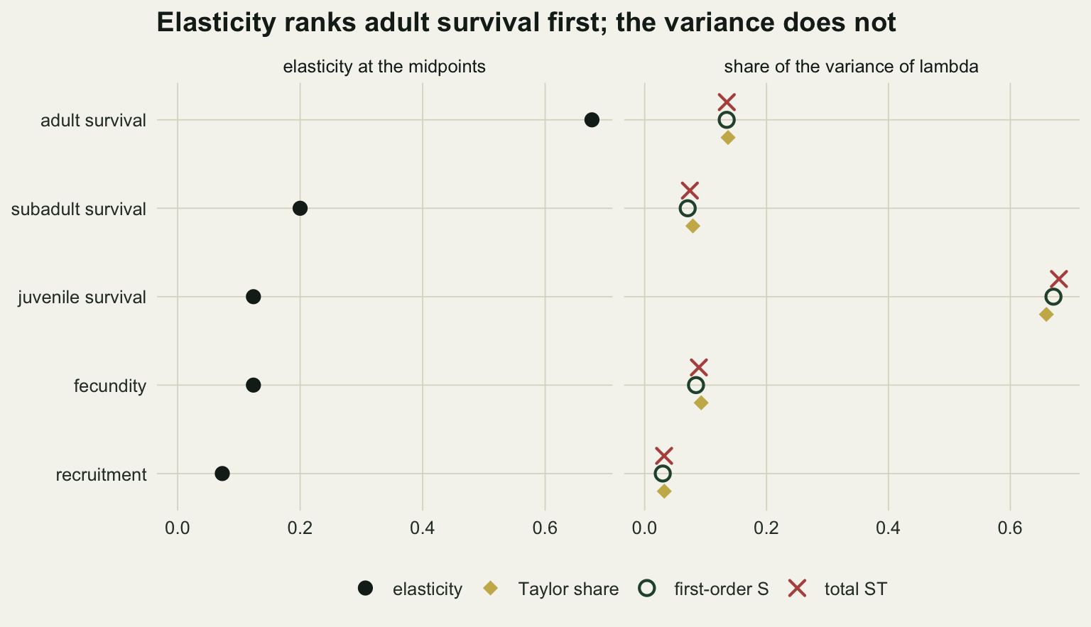
The first-order estimate needs a centred output
Those first-order numbers are from the centred estimator. The uncentred one, which is the formula as Saltelli and colleagues write it and as it comes out when coded by hand from the paper, has the same expectation but a very different spread from one replicate to the next.
shift_sd  <- sd_m[, "shift"]
raw_rng   <- apply(rep_m[, "S_raw", ], 1, range)
raw_neg   <- mean(rep_m[, "S_raw", ] < 0)
set.seed(5105)
lam_big <- lam_fast(draw_unif(2e5, lo_m, hi_m))
ratio_m <- mean(lam_big) / sd(lam_big)
pred_sd <- ratio_m * sqrt(2 * mean_m[, "ST"] / n_base)
sd_se_rel <- 1 / sqrt(2 * (n_rep - 1))
pred_gap <- shift_sd / pred_sd - 1
shift_z <- abs(mean_m[, "shift"]) / (shift_sd / sqrt(n_rep))
stopifnot(max(abs(rep_m[, "S_raw", ] - rep_m[, "S_cen", ] - rep_m[, "shift", ])) < 1e-10,
          max(shift_z) < 2)
print(round(cbind(sd_raw = sd_m[, "S_raw"], sd_centred = sd_m[, "S_cen"],
                  sd_ST = sd_m[, "ST"], predicted_shift_sd = pred_sd), 3))
sd_raw sd_centred sd_ST predicted_shift_sd
sj 0.238 0.011 0.010 0.218
ss 0.073 0.004 0.001 0.072
g 0.048 0.003 0.001 0.047
sa 0.104 0.006 0.002 0.097
f 0.082 0.005 0.002 0.079At N = 8000, the uncentred first-order estimate for juvenile survival has a standard deviation of 0.238 over replicates and ranges from 0.05 to 1.29, above one; 15 per cent of all uncentred estimates over the five rates are negative. The centred estimate for the same rate has a standard deviation of 0.011, and the total index 0.010. The averages over replicates agree: 0.685 uncentred against 0.671 centred for juvenile survival, and on every rate the difference between the two averages is less than 1.7 of its own Monte Carlo standard errors.
The cause is a single term. The uncentred estimate equals the centred one plus m * mean(f(AB_i) - f(A)) / V, where m is the mean output and V its variance (the stopifnot line checks the identity on every replicate). That term has expectation zero, because f(AB_i) and f(A) have the same distribution, and its variance follows from the definition of the total index: f(A) - f(AB_i) has mean square 2 V ST_i, so the term has a standard deviation of about (m / sd(Y)) * sqrt(2 ST_i / N). For lambda the ratio m / sd(Y) is 16.7: a growth rate near 1.09 with a standard deviation of 0.066 over the input box. The formula predicts a standard deviation of 0.218 for juvenile survival against a measured standard deviation of the shift term of 0.239 (a different quantity from the 0.238 of the uncentred estimate itself, though close to it because the centred part barely moves), and 0.097 against 0.104 for adult survival. A standard deviation from 200 replicates is itself uncertain by about 5 per cent; on this seed the measured values lie above the predictions on all five rates, by 0.9 to 9.7 per cent, the largest gap 1.9 of those standard errors. The Jansen total estimator uses only differences of outputs, so the mean never enters it.
The practical rule is to centre the output before using the first-order formula, or to use eta squared, and in either case to report a second estimate beside it: a single uncentred first-order index at a few thousand rows can be almost anything for an output whose mean is large against its spread.
The problem is known to the authors of the common software. SALib, the Python library, in version 1.6.0 (analyze/sobol.py) standardises the model output, subtracting its mean and dividing by its standard deviation, before its first-order and total estimators run, with a comment in the source that gives non-centred outputs as the reason. The R package sensitivity, in version 1.31.0, codes this first-order estimator as sobol2007 and does not centre the output; its help page tells the user to centre a largely non-centred output first and names soboljansen, sobolmartinez and sobolEff as free of the problem. The estimator bites when it is coded by hand from the paper, or when sobol2007 is given the raw output.
shift_long <- rbind(
  data.frame(rate = rep(rownames(mean_m), n_rep), version = "uncentred",
             val = as.vector(rep_m[, "S_raw", ])),
  data.frame(rate = rep(rownames(mean_m), n_rep), version = "centred",
             val = as.vector(rep_m[, "S_cen", ])))
shift_long$rate <- factor(rate_lab[shift_long$rate], rev(rate_lab[c("sa", "ss", "sj", "f", "g")]))
shift_long$version <- factor(shift_long$version, c("uncentred", "centred"))
eta_df <- data.frame(rate = factor(rate_lab[names(nom_m)], levels(shift_long$rate)), val = eta_m)
set.seed(5111)
shift_long$y_pos <- as.numeric(shift_long$rate) +
  ifelse(shift_long$version == "centred", 0.18, -0.18) + runif(nrow(shift_long), -0.1, 0.1)
eta_df$y_pos <- as.numeric(eta_df$rate)
ggplot(shift_long, aes(val, y_pos, colour = version)) +
  geom_vline(xintercept = 0, colour = te_body, linewidth = 0.4) +
  geom_point(size = 0.9, alpha = 0.45) +
  geom_point(data = eta_df, aes(val, y_pos), inherit.aes = FALSE, shape = 18,
             size = 3.6, colour = te_ink) +
  scale_y_continuous(breaks = seq_along(levels(shift_long$rate)),
                     labels = levels(shift_long$rate)) +
  scale_colour_manual(values = c(te_rust, te_forest), name = NULL) +
  guides(colour = guide_legend(override.aes = list(size = 3, alpha = 1))) +
  labs(x = "estimated first-order index", y = NULL,
       title = "Same design, same runs: the mean of lambda is the noise") +
  theme_datasheet() +
  theme(legend.position = "bottom")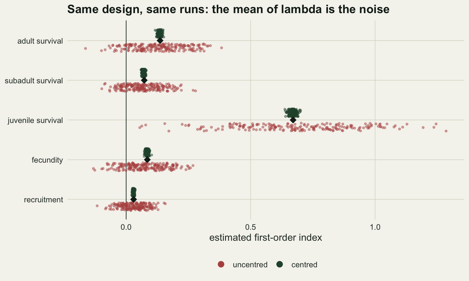
A yield curve at its peak
The second model is the equilibrium of the Schaefer surplus production model that Surplus production models in R fits to catch and index data. With fishing effort E and catchability q, the fishing mortality is qE, the equilibrium biomass is K (1 - qE / r) and the equilibrium yield is qE times that; when qE exceeds r there is no positive equilibrium and the stock is fished out, so the yield is set to zero. The effort is fixed at 100 days, which is the effort giving maximum sustainable yield at the midpoints of the ranges for r (0.2 to 0.8), K (800 to 1200 tonnes) and q (0.001 to 0.004 per day): qE is then r / 2, as in the fishing mortality at MSY of that post.
At that point the elasticities can be written down. With h = qE / r, the yield is K r h (1 - h), and differentiating its logarithm gives an elasticity of h / (1 - h) for r, one for K, and 1 - h / (1 - h) for q. At h = 1/2 these are one, one and zero: the yield sits at the top of its curve in q, so a small change in catchability does nothing. The Taylor share therefore gives q nothing at all, whatever its range.
effort <- 100
yield_eq <- function(x) pmax(x[, "q"] * effort * x[, "K"] * (1 - x[, "q"] * effort / x[, "r"]), 0)
yield_nf <- function(x) x[, "q"] * effort * x[, "K"] * (1 - x[, "q"] * effort / x[, "r"])
lo_w <- c(r = 0.2, K = 800, q = 0.001)
hi_w <- c(r = 0.8, K = 1200, q = 0.004)
nom_s <- (lo_w + hi_w) / 2
h_nom <- nom_s[["q"]] * effort / nom_s[["r"]]
stopifnot(abs(h_nom - 0.5) < 1e-12)

el_s <- setNames(elast_fd(yield_eq, nom_s), names(nom_s))
el_exact <- c(r = h_nom / (1 - h_nom), K = 1, q = 1 - h_nom / (1 - h_nom))
stopifnot(max(abs(el_s - el_exact)) < 1e-6)
taylor_share <- function(lo, hi) {
  cv <- (hi - lo) / (sqrt(12) * (lo + hi) / 2)
  (el_s * cv)^2 / sum((el_s * cv)^2)
}
cv_w  <- (hi_w - lo_w) / (sqrt(12) * nom_s)
tay_w <- taylor_share(lo_w, hi_w)

grp <- list(1, 2, 3, c(1, 3))
set.seed(5106)
rep_w  <- replicate(n_rep, sobol_run(yield_eq, lo_w, hi_w, n_base, grp))
mean_w <- apply(rep_w, 1:2, mean)
sd_w   <- apply(rep_w, 1:2, sd)
set.seed(5107)
eta_w <- rowMeans(replicate(5, eta_sq(yield_eq, lo_w, hi_w, 2e5)))

int_q   <- mean_w[["q", "ST"]] - mean_w[["q", "S_cen"]]
int_rq  <- mean_w[["r:q", "S_cen"]] - mean_w[["r", "S_cen"]] - mean_w[["q", "S_cen"]]
sum_s_w <- sum(mean_w[c("r", "K", "q"), "S_cen"])
mcse_w  <- max(sd_w[, c("S_cen", "ST")]) / sqrt(n_rep)
rq_check <- abs((1 - mean_w[["r:q", "S_cen"]]) - mean_w[["K", "ST"]])
stopifnot(rq_check < 0.005)

qe_lo <- lo_w[["q"]] * effort
qe_hi <- hi_w[["q"]] * effort
box_area <- (hi_w[["r"]] - lo_w[["r"]]) * (qe_hi - qe_lo)
tri_area <- integrate(function(r_val) pmax(qe_hi - pmax(r_val, qe_lo), 0),
                      lo_w[["r"]], hi_w[["r"]])$value
p_zero_exact <- tri_area / box_area
set.seed(5108)
x_big <- draw_unif(1e6, lo_w, hi_w)
y_big <- yield_eq(x_big)
p_zero <- mean(y_big == 0)
p_zero_se <- sqrt(p_zero * (1 - p_zero) / length(y_big))
p_zero_z <- (p_zero - p_zero_exact) / p_zero_se
var_ratio <- var(yield_nf(x_big)) / var(y_big)
stopifnot(abs(p_zero_exact - 1 / 9) < 1e-6, abs(p_zero_z) < 4)
print(round(cbind(taylor = c(tay_w, "r:q" = NA), S_centred = mean_w[, "S_cen"],
                  eta_sq = c(eta_w, "r:q" = NA), ST = mean_w[, "ST"]), 3))
taylor S_centred eta_sq ST
r 0.9 0.747 0.745 0.935
K 0.1 0.042 0.043 0.055
q 0.0 0.025 0.025 0.203
r:q NA 0.946 NA 0.959The Taylor share is 0.9 for r, 0.1 for K and zero for q; r dominates because its range has a CV of 0.346 against 0.115 for K, both at elasticity one. The total index of catchability is 0.203. Its first-order index is 0.025 by the centred estimator and 0.025 by eta squared, so 0.178 of the output variance is catchability acting through its interactions. The Monte Carlo standard error of every index averaged here is at most 0.0010.
The interaction has a partner. Treating r and q as one group, the same first-order estimator gives the share of the pair, 0.946; taking away the two first-order indices leaves 0.174 for the interaction of r with q, nearly all of the 0.178. With three inputs the pair r and q is everything except K, so one minus the pair’s share must equal the total index of K, and the two come from different formulas; they agree, 0.0544 against 0.0546. The reason is visible in the formula for h. The catchability that gives the largest yield is q = r / (2 E), so whether a given q is too high or too low depends on r: for a slow-growing stock a high catchability overfishes it, and for a fast-growing one the same catchability is still short of the peak. Averaged over the r range the effect of q nearly cancels, while at a single value of r it moves the yield up or down, as the figure below shows. The first-order indices of the three inputs sum to 0.813 (0.814 by eta squared).
The same formula also sets the yield to zero in part of the box, wherever qE is above r: a slow stock at high catchability. That share needs no simulation. At fixed effort qE is uniform from 0.1 to 0.4 and r from 0.2 to 0.8, so the draws with qE above r fill a triangle of area 0.02 inside a rectangle of area 0.18, a share of one ninth, 0.1111. A million draws reproduce it, 0.1105 with a Monte Carlo standard error of 0.0003 (2.0 standard errors off, which on one seed is no discrepancy).
q_grid <- seq(lo_w[["q"]], hi_w[["q"]], length.out = 200)
slice_df <- do.call(rbind, lapply(c(0.3, 0.5, 0.7), function(r_val) {
  x_sl <- cbind(r = r_val, K = 1000, q = q_grid)
  data.frame(q = q_grid, yield = yield_eq(x_sl), line = sprintf("r = %.1f", r_val))
}))
set.seed(5109)
x_cm <- draw_unif(2e5, lo_w, hi_w)
y_cm <- yield_eq(x_cm)
q_cls <- cut(x_cm[, "q"], quantile(x_cm[, "q"], 0:100 / 100), include.lowest = TRUE)
cm_df <- data.frame(q = as.vector(tapply(x_cm[, "q"], q_cls, mean)),
                    yield = as.vector(tapply(y_cm, q_cls, mean)), line = "mean over r and K")
cm_range <- range(cm_df$yield)
slice_df <- rbind(slice_df, cm_df)
slice_df$line <- factor(slice_df$line, c("r = 0.3", "r = 0.5", "r = 0.7", "mean over r and K"))
ggplot(slice_df, aes(q, yield, colour = line, linewidth = line)) +
  geom_vline(xintercept = nom_s[["q"]], linetype = "dashed", colour = te_body, linewidth = 0.4) +
  geom_line() +
  scale_colour_manual(values = c(te_rust, te_gold, te_forest, te_ink), name = NULL) +
  scale_linewidth_manual(values = c(0.9, 0.9, 0.9, 1.4), name = NULL) +
  labs(x = "catchability q per day (effort fixed at 100 days)",
       y = "equilibrium yield (tonnes)",
       title = "The best catchability moves with r") +
  theme_datasheet() +
  theme(legend.position = "bottom")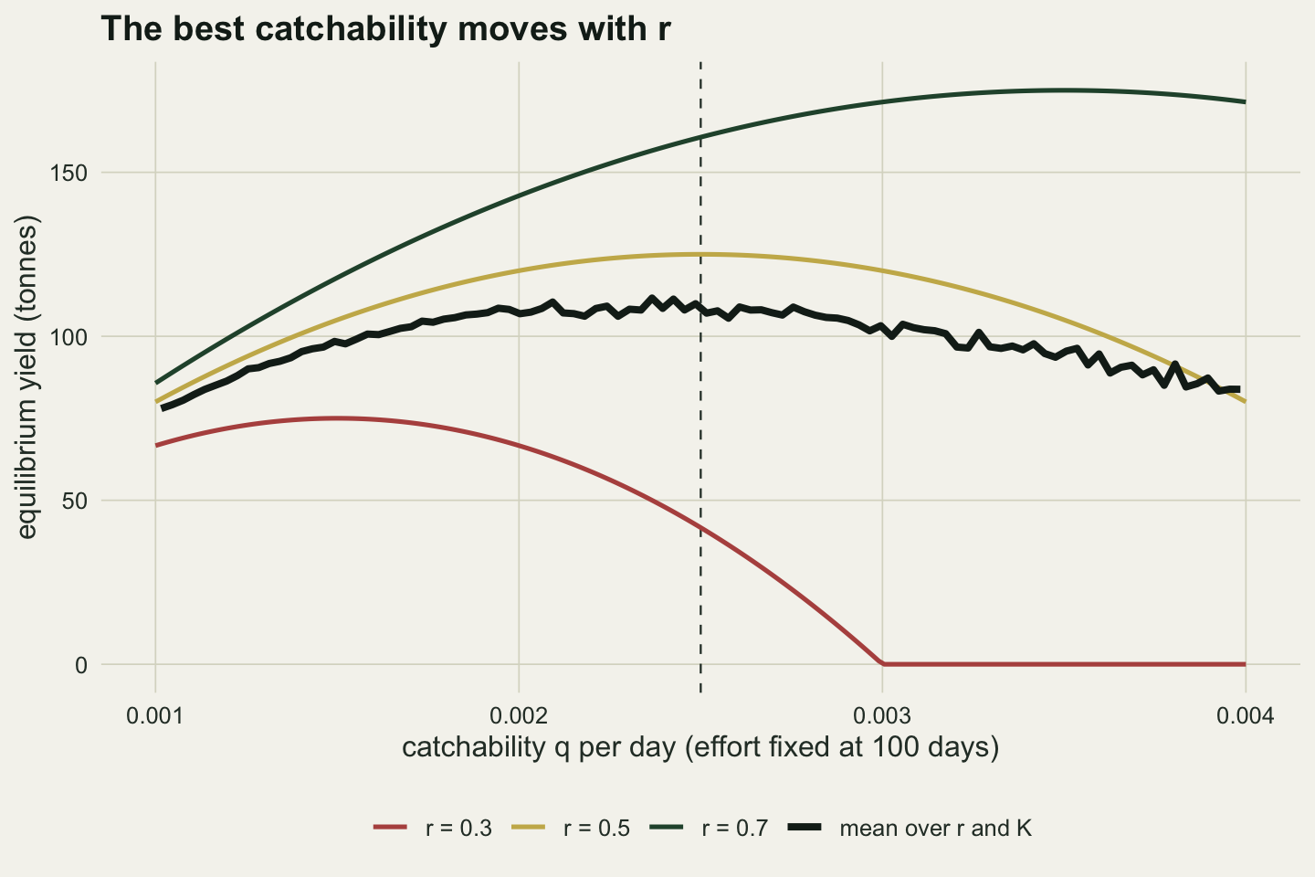
The mean yield over all draws in each class of q moves only between 78 and 112 tonnes across the whole range of catchability, while the slice at r = 0.3 falls to zero from q = 0.003 on, where qE reaches r, and the slice at r = 0.7 is still rising at the midpoint. That nearly flat black line is what the first-order index of q measures, and the fan of coloured lines is what its total index adds.
The collapse is not the source
The zero yield is a kink in the model, and it is tempting to credit the interaction to it. Two checks separate the two. The first removes the floor and lets the yield go negative where the stock would be fished out: a diagnostic, not a model. The second keeps the floor but uses narrower ranges, 30 per cent either side of the same midpoints for all three inputs, so r runs from 0.35 to 0.65, K from 700 to 1300 and q from 0.00175 to 0.00325. Then qE never exceeds r, and the Taylor share is one half each for r and K.
set.seed(5110)
rep_nf  <- replicate(50, sobol_run(yield_nf, lo_w, hi_w, n_base))
mean_nf <- apply(rep_nf, 1:2, mean)
mcse_nf <- sd(rep_nf["q", "ST", ]) / sqrt(dim(rep_nf)[3])

lo_e <- c(r = 0.35, K = 700, q = 0.00175)
hi_e <- c(r = 0.65, K = 1300, q = 0.00325)
stopifnot(all.equal(unname((lo_e + hi_e) / 2), unname(nom_s)),
          hi_e[["q"]] * effort < lo_e[["r"]])
tay_e <- taylor_share(lo_e, hi_e)
set.seed(5112)
rep_e  <- replicate(n_rep, sobol_run(yield_eq, lo_e, hi_e, n_base, grp))
mean_e <- apply(rep_e, 1:2, mean)
sd_e   <- apply(rep_e, 1:2, sd)
set.seed(5113)
eta_e <- rowMeans(replicate(5, eta_sq(yield_eq, lo_e, hi_e, 2e5)))
int_rq_e <- mean_e[["r:q", "S_cen"]] - mean_e[["r", "S_cen"]] - mean_e[["q", "S_cen"]]
gap_e <- mean_e[c("r", "K", "q"), "ST"] - tay_e
mcse_e <- max(sd_e[, c("S_cen", "ST")]) / sqrt(n_rep)
rq_check_e <- abs((1 - mean_e[["r:q", "S_cen"]]) - mean_e[["K", "ST"]])
st_w <- mean_w[c("r", "K", "q"), "ST"]
st_e <- mean_e[c("r", "K", "q"), "ST"]
stopifnot(rq_check_e < 0.005,
          identical(names(sort(st_w, decreasing = TRUE)), c("r", "q", "K")),
          identical(names(sort(st_e, decreasing = TRUE)), c("r", "K", "q")),
          st_e[["r"]] - st_e[["K"]] < 0.5 * (st_w[["r"]] - st_w[["q"]]))
print(round(rbind(no_floor_ST = mean_nf[, "ST"], narrow_taylor = tay_e,
                  narrow_S = mean_e[c("r", "K", "q"), "S_cen"], narrow_eta = eta_e,
                  narrow_ST = mean_e[c("r", "K", "q"), "ST"]), 3))
r K q
no_floor_ST 0.926 0.028 0.322
narrow_taylor 0.500 0.500 0.000
narrow_S 0.528 0.380 0.013
narrow_eta 0.528 0.380 0.013
narrow_ST 0.606 0.399 0.075Without the floor, over 50 replicates, the total index of catchability rises to 0.322 (Monte Carlo standard error 0.002) from 0.203, and on the million draws above the yield variance without the floor is 2.2 times that with it: the floor flattens part of the yield surface and removes variance, and the interaction is there without it. On the narrower box, where no draw is fished out (the stopifnot line checks that the highest qE is below the lowest r), catchability still has a total index of 0.075 against a first-order index of 0.013 (0.013 by eta squared), and the r by q interaction is 0.059; the check against the total index of K holds here too, 0.3993 against 0.3989. The collapse probability is worth reporting, because a yield of zero matters to a manager more than its share of a variance does, but here it is not what makes catchability matter.
The ranges are part of the answer
The narrow box also reorders the inputs. Carrying capacity moves ahead of catchability, with total indices of 0.399 against 0.075, where the wide box had 0.055 against 0.203. Growth rate keeps first place, with 0.606 against 0.935 in the wide box, but with a much smaller lead. The Taylor share splits r and K evenly, and their total indices lie off it by up to 0.106 (Monte Carlo standard error at most 0.0008). Nothing about the fishery changed between the two; only the stated uncertainty about it did. Every index here is a statement about the input ranges as much as about the model, and a range written down without a source is an assumption that the ranking then inherits.
box_lab <- c("wide ranges", "narrow ranges (30 per cent)")
harv_long <- do.call(rbind, lapply(1:2, function(b) {
  tay_b <- if (b == 1) tay_w else tay_e
  mean_b <- if (b == 1) mean_w else mean_e
  rbind(data.frame(box = box_lab[b], input = names(tay_b), measure = "Taylor share", val = tay_b),
        data.frame(box = box_lab[b], input = names(tay_b), measure = "first-order S",
                   val = mean_b[names(tay_b), "S_cen"]),
        data.frame(box = box_lab[b], input = names(tay_b), measure = "total ST",
                   val = mean_b[names(tay_b), "ST"]))
}))
input_lab <- c(r = "growth rate r", K = "carrying capacity K", q = "catchability q")
harv_long$input <- factor(input_lab[harv_long$input], rev(input_lab))
harv_long$measure <- factor(harv_long$measure, c("Taylor share", "first-order S", "total ST"))
harv_long$box <- factor(harv_long$box, box_lab)
harv_long$y_pos <- as.numeric(harv_long$input) + off_meas[as.character(harv_long$measure)]
ggplot(harv_long, aes(val, y_pos, colour = measure, shape = measure)) +
  geom_point(size = 3.2, stroke = 1.1) +
  facet_wrap(~ box) +
  scale_y_continuous(breaks = seq_along(levels(harv_long$input)), labels = levels(harv_long$input)) +
  scale_colour_manual(values = c(te_gold, te_forest, te_rust), name = NULL) +
  scale_shape_manual(values = c(18, 1, 4), name = NULL) +
  scale_x_continuous(limits = c(0, 1), breaks = c(0, 0.25, 0.5, 0.75, 1),
                     labels = c("0", "0.25", "0.5", "0.75", "1")) +
  labs(x = "share of the variance of equilibrium yield", y = NULL,
       title = "Zero elasticity, a fifth of the variance") +
  theme_datasheet() +
  theme(legend.position = "bottom", panel.spacing = unit(1.6, "lines"))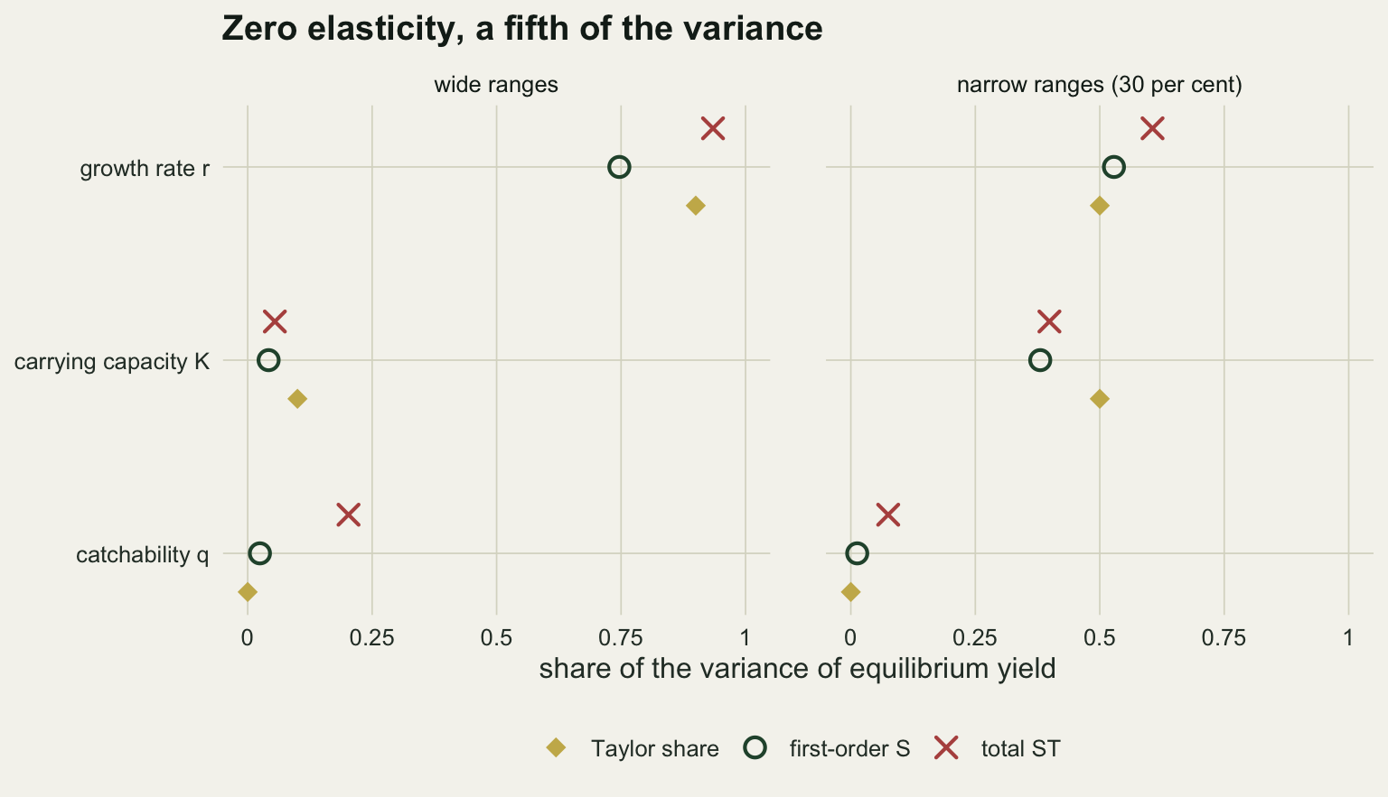
What to report
Report the input ranges, where each came from, and the distribution drawn within them. A uniform range of 0.1 to 0.5 for juvenile survival is a claim about the state of knowledge, and it decided the matrix ranking above more than the model did.
Compute the Taylor share, (e_i CV_i)^2 divided by its sum, before any Sobol index, and report it beside them. It costs a handful of model runs. If the total indices agree with it, as they did for lambda to within 0.021, say that the ranking follows from elasticity and input spread and the Sobol analysis has confirmed it; do not present the ranking as something the indices found. If they disagree, as for catchability, the disagreement is the finding, and the gap between total and first-order index says how much of it is interaction.
Report both indices for every input with their Monte Carlo standard errors, from replicate runs or a bootstrap over the rows, together with N and the number of model runs. Compute the first-order index with the output centred, and give a second estimate from a different construction, such as eta squared over classes of the input. An uncentred first-order index from one run of a few thousand rows should not be reported at all for an output whose mean is large against its spread.
Where the input ranges cross a regime boundary of the model, such as a stock fished out, report the share of draws on the far side of it. It is a quantity a variance index does not show.
Honest limits
The inputs are independent and uniform. Estimates of vital rates are often correlated, because they come out of the same capture-recapture fit, and the rates themselves co-vary from year to year; the post on checking a reintroduction analysis measures what the second kind does to a projection. With dependent inputs the variance no longer splits into one term per input plus interactions, and the indices here lose their meaning; variants for dependent inputs exist and were not tried.
Both models are deterministic, and the outputs are an asymptotic growth rate and an equilibrium yield. A stochastic projection adds variance that belongs to no input, and a transient or finite-horizon output can be far more nonlinear in its inputs than lambda is.
Variance is the only summary. The yield in the wide box is skewed, with a spike at zero, and an index of its variance says nothing about the probability of collapse; a variance-based index can rank an input low whose extreme values are the ones that matter.
The Taylor share was taken to first order at the midpoints only. A second-order expansion would give catchability a share from the curvature at the peak, and was not computed; nor were the matrix ranges widened to find where the first-order share stops holding. The small gap for juvenile survival, the rate with the widest range, suggests where that would start.
Two models, one set of ranges for the matrix and two for the harvest model, are a demonstration, not a survey. The Sobol indices themselves, the pick-freeze design and the estimators are standard; the shift term that makes the uncentred first-order estimate noisy is derived and checked here in one line, and the post does not claim it as new; centring the output is the remedy the two software packages named above already apply or document.
References
Sobol IM 2001 Mathematics and Computers in Simulation 55(1-3):271-280 (10.1016/S0378-4754(00)00270-6)
Saltelli A, Annoni P, Azzini I, Campolongo F, Ratto M, Tarantola S 2010 Computer Physics Communications 181(2):259-270 (10.1016/j.cpc.2009.09.018)
Jansen MJW 1999 Computer Physics Communications 117(1-2):35-43 (10.1016/S0010-4655(98)00154-4)
Mills LS, Doak DF, Wisdom MJ 1999 Conservation Biology 13(4):815-829 (10.1046/j.1523-1739.1999.98232.x)
Caswell H 2001 Matrix Population Models, 2nd ed (ISBN 978-0-87893-096-8)